Anchor-Free Object Detection with Scale-Aware Networks for Autonomous Driving

Abstract

Current anchor-free object detectors do not rely on anchors and obtain comparable accuracy with anchor-based detectors. However, anchor-free object detectors that adopt a single-level feature map and lack a feature pyramid network (FPN) prior information about an object’s scale; thus, they insufficiently adapt to large object scale variation, especially for autonomous driving in complex road scenes. To address this problem, we propose a divide-and-conquer solution and attempt to introduce some prior information about object scale variation into the model when maintaining a streamlined network structure. Specifically, for small-scale objects, we add some dense layer jump connections between the shallow high-resolution feature layers and the deep high-semantic feature layers. For large-scale objects, dilated convolution is used as an ingredient to cover the features of large-scale objects. Based on this, a scale adaptation module is proposed. In this module, different dilated convolution expansion rates are utilized to change the network’s receptive field size, which can adapt to changes from small-scale to large-scale. The experimental results show that the proposed model has better detection performance with different object scales than existing detectors.

1. Introduction

Object detection is an essential element in fields such as autonomous driving [1,2,3] and robotics [4] and has, in recent years, drawn the attention of many researchers. This has led to substantial developments in the creation of existing object detection techniques. In particular, with the development and application of deep learning [5] and other technologies, newer object detection techniques continue to show significantly improving performances over their predecessors.

Object detectors can be divided into one-stage and two-stage pipelines [6,7]. The early deep detection recurrent convolutional neural network (R-CNN) model [8] and others [9,10,11] are traditional methods that follow a sliding window-based pipeline. Subsequently, two-stage detectors, including SPPNet [10], Fast R-CNN [9], Faster R-CNN [11] and others, were developed and continued to follow this route. Two-stage detectors have high detection accuracy but have high computational complexity as well. To address this issue, many one-stage detectors were subsequently proposed, such as the SSD [12,13,14] and YOLO series [15,16]. Object detectors can also be divided into anchor-based and anchor-free methods. Following the proposal of the anchor concept in object detection with Faster R-CNN [11], many two- and one-stage detectors were subsequently developed. A preset box with different scales and ratios at the anchor point can provide some prior information about the object’s scale. By appropriately setting the parameters of the anchor, the prediction space of the model can be reduced. In addition, the anchor box can alleviate the problem of unbalanced category distribution between the foreground and background in object detection.

However, current anchor-based detection methods are limited by a number of deficiencies. First, the performance of the detector is sensitive to the anchor parameters, but adjusting these parameters can be complicated. Second, the detection model requires additional preprocessing operations such as anchor definitions and postprocessing operations such as nonmaximum suppression (NMS), thus increasing the model’s computational complexity.

With the goal of addressing the shortcomings of anchor-based detection, some anchor-free detectors have been subsequently proposed, including CornerNet [17], FCOS [18], CenterNet [19], and ATSS [20]. FCOS and ATSS implement a feature pyramid network (FPN) [21] with multilevel feature maps which can alleviate the object scale variation problem. However, the FPN module, which uses multiple feature layers for prediction, adds complexity to the network structure. Unlike FCOS and ATSS, CornerNet, CenterNet, and other models that lack the FPN structure only use a single-level feature layer for prediction. The detectors thus have a streamlined structure but lack prior information about the object’s scale variation (both the predefined anchor boxes and multilevel feature maps). The size of the receptive field on the single-level feature is relatively fixed, and it is difficult to ensure the scale adaptability of the model by directly inputting only the single-level feature map. As a result, these modules perform poorly in scenarios with large target scale variations, such as in complex road scene object detection for autonomous driving. As shown in Figure 1, the target scale varies widely on both camera image datasets in complex road scenes, which are KITTI [22] and BDD100K [23].

One question raised is whether multiscale detection can be performed using only single-level features without an FPN module or multilevel feature maps. In this paper, to address the insufficient adaptability of anchor-free models lacking the FPN module to large object scale variation in complex scene object detection, we propose a divide-and-conquer solution, introduce some prior information about object scale variation into such a model, and finally propose the scale-aware CenterNet, or SA-CenterNet. Specifically, to adapt to small-scale object detection, an improved high-resolution feature extraction network is adopted. This network adds some dense layer jump connections between the shallow high-resolution feature layers and the deep layers; we argue that these shallow high-resolution features are helpful for the detection of small objects. To adapt to large-scale object detection, dilated convolution [24] is utilized as an ingredient to cover the features of large-scale objects. To overcome the issue that the target varies greatly from small-scale to large-scale and maintain high calculation efficiency, a parallel structure with multiple branches and different dilation rates is designed. The varying dilated convolution rate on a single-level feature map can be regarded as compensation for the size variation of the target. Finally, a large number of experiments are performed on two publicly used road scene camera image datasets for autonomous driving. The experimental results show that the proposed model has better performance in detecting different scales than the original classic CenterNet and other similar recently proposed anchor-free detectors. The effectiveness of each module included in the model is verified by ablation experiments.

To summarize, our paper makes the following contributions:

•

We propose a divide-and-conquer strategy for anchor-free and multiscale object detection without a feature pyramid structure.

•

We present a densely connected high-resolution network and a scale adaptation module to improve the performance of multiscale detection.

•

We conduct extensive experiments on publicly available autonomous driving datasets to compare some recently advanced detectors and demonstrate the effectiveness of our proposed approach.

2. Related Work

Anchor-free Object Detection. A number of anchor-free detectors have been proposed recently to overcome the weaknesses of the anchor design in previous anchor-based detectors. YOLO [15] first predicts the bounding box’s location based on cells in the image, not on the additional predefined anchor box. CornerNet [17] models object detection as the problem of predicting the upper-left and lower-right corners of the object, but the processing for this corner matching is highly computationally complex. To avoid corner matching processing, CenterNet [19] and FCOS [18] were subsequently proposed; both model object detection as the problem of predicting the center and size of the object. The difference between the two models is that CenterNet predicts the heatmaps of the center of the object, while FCOS predicts the centrality of the center with a fully convolutional architecture. Another recently proposed model is ATSS [20], which implements a novel adaptive training sample selection strategy that can bridge the gap between anchor-based and anchor-free detection.

Multiscale Object Detection. In the early stages, image pyramids [25,26] were used to overcome the problem of multiscale changes in the target. Due to the need to repeatedly perform feature extraction and classification on images of different scales, image pyramid processing significantly increases the computational complexity of object detection. In the era of deep learning, a feature pyramid module [21] was proposed to address the object multiscale variation problem and avoid the very large computational costs of the image pyramid module. Subsequently, different improved feature fusion methods based on the FPN were proposed to better extract multiscale information [27,28,29,29]. Trident networks [30] generate scale-specific feature maps through a parallel multibranch architecture in which each branch shares the same transformation parameters but with different receptive fields. Pang et al. [31] introduced self-interaction modules to adaptively extract multiscale information from specific levels by using average pooling to enlarge the receptive fields. The difference between our proposed method and the above methods is that we propose new strategies for improving small object, large object, and object scale change detection in an anchor-free architecture. YOLOF [32] only utilizes single-layer features without dominated feature pyramid networks (FPN) and the success of FPN is due to its divide-and-conquer solution to the optimization problem rather than a multiscale feature fusion. In this paper, we follow this idea and propose a method to improve the scale adaptability of anchor-free detectors that only utilize one-layer input features.

3. Materials and Methods

Inspired by YOLOF [32], we maintained the one-level feature layer and then designed a scale-aware and anchor-free object detector named SA-CenterNet. Specifically, for small-scale object detection, we designed densely connected high-resolution networks; for large-scale object detection, we utilized dilated convolution [24] as an element; to mitigate the issue of targets greatly varying from small to large scale, we propose the scale adaptation module. The overall architecture diagram is shown in Figure 2.

3.1. Preliminary

High-Resolution Networks. Recently, the work in [33] argued that deep high-resolution representation benefits visual recognition, and they proposed a high-resolution network (HRNet) that connects high-to-low resolution convolution streams in parallel and repeatedly exchanges the information across different resolutions. The benefit of this is that the deep high-resolution representation is semantically richer and spatially more precise, and parallel processing makes it efficient. As illustrated in Figure 3, HRNet outputs $N_{4i}$, defined as

$$N_{4i}=f_i(\sum _j{g}_{ij}\left(N_{3j}\right))$$

(1)

$N_{lr}$ represents the feature map obtained during the l-th stage with a resolution index r, and $f(•)$ and $g(•)$ represent the transform layers of the networks.

CenterNet. CenterNet [19] is a representative anchor-free object detector. This detector models the target detection as the location of the target center point and the regression of the length and width of the target, given only a single-level feature map. Specifically, the location of the target center position is achieved by predicting the center point heatmap and taking the maximum local response. The length/width of the object is decomposed into the distance from the center of the object to the boundary of the bounding box.

3.2. Densely Connected High-Resolution Networks

HRNet maintains high-resolution convolutional features and exchanges high-level and low-level information in parallel; consequently, it can achieve better performance on some computer vision tasks. In this paper, we propose a more densely connected high-resolution network based on HRNet. Inspired by DenseNet [34] and PANet [35], we further connect the former high-resolution convolutional feature maps to the later low-resolution convolutional feature maps to obtain and use the high-resolution convolutional features of the former more effectively. These densely connected high-resolution networks contribute to the detection of small-scale objects.

In this paper, our densely connected high-resolution network output ${\tilde{N}}_{4i}$ is defined as

$${\tilde{N}}_{4i}=f_i(\sum _j{g}_{ij}\left(N_{3j}\right)+{\varphi }_{i1}\left(N_{21}\right)+{\varphi }_{i2}\left(N_{22}\right)),$$

(2)

$N_{lr}$ represents the feature map obtained during the l-th stage with a resolution index r, $f(•)$ and $g(•)$ represent the transform layers of the networks, and $\varphi (•)$ represents the transform layers of the networks, consisting of a convolution layer, a batch normalization layer, and a ReLU layer.

3.3. Scale Adaptation Module

We note that CenterNet and other detectors that lack the FPN module only use a one-level feature map to predict the object’s category and size. However, the receptive field of one-level feature maps is fixed; consequently, these detectors have limited performance when the object’s scale varies over a large range. Inspired by the techniques proposed in [24,30], we use dilated convolution to enlarge the receptive field size to cover large-scale objects. In addition, we use different dilated convolution expansion rates to change the receptive field size, which can then adapt to changes in the object scale. To maintain efficiency, we adopt a parallel structure; given an input one-level feature map $\mathbf{X}$, the scale-aware module calculates the scale-aware feature map $\mathbf{Y}$ as

$$\mathbf{X}={\tilde{N}}_{41}\oplus U({\tilde{N}}_{42})\oplus U({\tilde{N}}_{43})\oplus U({\tilde{N}}_{44}),$$

(3)

$$\mathbf{Y}=f(\mathbf{X}\oplus D_1(\mathbf{X})\oplus D_2(\mathbf{X})\oplus D_3(\mathbf{X})),$$

(4)

where $U(•)$ is an upsampling operation, $D_1(•)$, $D_2(•)$, and $D_3(•)$ represent the dilated convolution module with different expansion rates n⊕ represents the concatenate operation, and $f(•)$ represents the transform layers that contain the convolution layer for reducing the number of channels, as illustrated in Figure 4. Each Scale-aware-n module consists of three consecutive convolutions: the first $1\times 1$ convolution applies channel reduction with a reduction rate of 4, then a $3\times 3$ convolution with dilation is used to increase the receptive field, and finally, a $1\times 1$ convolution expands the number of channels. Specifically, Scale-aware-0 represents a direct connection without any dilated convolution or other layers, Scale-aware-2 represents a dilated convolution module with expansion rate 2, Scale-aware-4 represents a dilated convolution module with expansion rate 4, and Scale-aware-6 represents a dilated convolution module with expansion rate 6. In each Scale-aware-n module, ConvM contains the convolution layer with a kernel size of $M\times M$, a batch normalization layer and a ReLU layer. Conv-dilation-n contains a dilated convolution module with expansion rate n, a batch normalization layer and a ReLU layer.

3.4. Model Training

The networks are trained by minimizing the following loss function:

$$\mathcal{L}={\mathcal{L}}_{heatmap}+{\lambda }_{offset}{\mathcal{L}}_{offset}+{\lambda }_{size}{\mathcal{L}}_{size}$$

(5)

where ${\mathcal{L}}_{heatmap}$ is the loss from predicting the heatmap of the center points, ${\mathcal{L}}_{offset}$ is the loss from predicting the offset of the center points, ${\mathcal{L}}_{size}$ is the loss from predicting the object size, and ${\lambda }_{offset}$ and ${\lambda }_{size}$ are the weight parameters. Specifically, ${\mathcal{L}}_{heatmap}$ is formed by (6) and ${\mathcal{L}}_{offset}$ and ${\mathcal{L}}_{size}$ are formed by an L1 loss, which is formed by (7). ${\lambda }_{offset}$ is set to 1, and ${\lambda }_{size}$ is set to $0.1$, as in CenterNet [19].

$${\mathcal{L}}_{heatmap}=-\sum _t{(1-p_t)}^{\gamma }log\left(p_t\right)$$

(6)

where $p_t$ is the t-th logit of the prediction on the heatmap for classification and $\gamma$ is a constant that is set to 4 in both CenterNet and our model.

$${\mathcal{L}}_{offset/size}=-1/N(\sum _i|L_i-\widehat{L_i}|)$$

(7)

$L_i$ is the i-th predicted offset or size and $\widehat{L_i}$ is the corresponding ground truth of the offset or size.

4. Experiments

4.1. Dataset and Evaluation Metrics

We conducted experiments on two publicly available autonomous driving datasets, KITTI [22] and BDD100K [23], which contain a large number of objects with large-scale changes. Specifically, the KITTI dataset was collected from different scenes in Karlsruhe during the daytime. We choose the 2D object detection data contained in KITTI, which consists of 7481 labeled images and then randomly reserved one-tenth of the original labeled dataset for testing. The chosen classes in KITTI include car, van, truck, pedestrian, person (sitting), cyclist, tram, and misc. BDD100K is a large-scale dataset that was released by the AI Lab of the University of Berkeley and collected from a complex road scene and contains sample images of various scenes under different venues, different weather conditions, and different lighting conditions. After processing, the dataset contains 70,000 images for training and 10,000 images for testing. The classes in BDD100K include car, bus, person, bike, truck, motor, train, rider, traffic sign, and traffic light.

For evaluation, we use the average precision (AP) and average recall (AR) metrics defined on the MS-COCO benchmark [36]. To verify the detection performance with objects at different scales, we use COCO-style $A{P}_s$, $A{P}_m$, $A{P}_l$, $A{R}_s$, $A{R}_m$, and $A{R}_l$ on objects of small (less than $32\times 32$), medium (from $32\times 32$ to $96\times 96$), and large (greater than $96\times 96$) sizes as the additional evaluation metrics. Given the total number of classes C, the class index c, the total number of objects of class c expected to be detected $N_c$, the number of objects of class c truly detected $P_c$, and the number of false alarms $M_c$, AP and AR are, respectively defined as:

$$AP=(\sum _{c=1}^C{P}_c/(P_c+M_c))/C$$

(8)

$$AR=(\sum _{c=1}^C{P}_c/N_c)/C$$

(9)

4.2. Implementation Details

We trained the network with the Adam optimizer, a starting learning rate of $1.25\times {10}^{-4}$, and a total batch size of 20 on 2 Nvidia A100 GPUs. The structural parameters of the baseline feature extraction network are consistent with the default settings of the original HRNet, and the downsampling rate of the output feature map is set to 4. Similar to CenterNet [19], we selected the top 100 response points from the heatmap and used the same settings as those in CenterNet for the remaining parameters. The networks were trained for 80 epochs to achieve convergence. In our experiment, the input KITTI image kept its original scale $1242\times 375$ due to its large aspect ratio, and the input BDD100k image was scaled to $512\times 512$ while maintaining a constant aspect ratio. We built our model based on the official implementation code of CenterNet.

4.3. Comparison with State-of-the-Art Methods

Here, we extensively evaluate our approach using a comparison to a variety of competing algorithms that contain the FPN module on the KITTI and BDD100K datasets. In these experiments, the input images are also scaled to $512\times 512$ while preserving the aspect ratio. All competing algorithms are implemented with MMDetection [37].

4.3.1. KITTI Dataset

We compared our approach with a number of typical anchor-based and anchor-free object detectors that contain FPN structures. As illustrated in

Table 1. Experimental results from different models on the KITTI dataset. All competing algorithms are implemented with MMDetection, and the default settings are used for the parameters.

Method	Backbone	AP	${\mathit{AP}}_{\mathit{s}}$	${\mathit{AP}}_{\mathit{m}}$	${\mathit{AP}}_{\mathit{l}}$	${\mathit{AR}}_{\mathit{s}}$	${\mathit{AR}}_{\mathit{m}}$	${\mathit{AR}}_{\mathit{l}}$
Faster R-CNN	ResNet-101-FPN	49.3	29.0	51.7	61.0	32.1	58.7	67.8
SSD	VGG16	36.5	27.3	37.0	45.4	34.8	47.7	59.6
YOLOv3	DarkNet53	36.5	32.3	39.1	40.3	38.1	47.0	49.5
FCOS	ResNet-101-FPN	51.3	41.9	53.3	56.3	48.5	62.9	67.8
CenterNet	HRNet-w48	52.8	52.8	55.4	53.3	58.1	61.8	65.7
ATSS	ResNet-101-FPN	54.2	47.7	54.8	60.1	53.3	64.9	72.8
Ours (SA-CenterNet)	HRNet-w48	56.9	53.6	59.4	57.4	58.2	66.0	67.9

, our model appears to achieve the best accuracy among all comparison models in all metrics. Notably, although our method uses a similar feature extraction network as CenterNet, the values of $AP@.5:.95$, $A{P}_s$, $A{P}_m$, $A{P}_l$, $A{R}_s$, $A{R}_m$, and $A{R}_l$ were higher; specifically, the model’s detection performance for small and large targets was improved by more than four points. It is worth noting that CenterNet was better than FCOS with FPN in the detection of small and medium objects. This may be because high-resolution feature networks contribute to small object detection. FCOS with FPN is better than CenterNet for the detection of large-scale objects. However, our model performs better than FCOS with FPN structure in the detection of both small and large objects. These results show the effectiveness of the optimized strategies for multiscale object detection in our method.

4.3.2. BDD100K Dataset

The results from the models with the BDD100K dataset are presented in

Table 2. Experimental results from different models with the BDD100K dataset. All competing algorithms are implemented with MMDetection, and the default settings are used for the parameters.

Method	Backbone	AP	${\mathit{AP}}_{\mathit{s}}$	${\mathit{AP}}_{\mathit{m}}$	${\mathit{AP}}_{\mathit{l}}$	${\mathit{AR}}_{\mathit{s}}$	${\mathit{AR}}_{\mathit{m}}$	${\mathit{AR}}_{\mathit{l}}$
Faster R-CNN	ResNet-101-FPN	17.7	1.6	23.0	45.3	1.4	35.3	54.0
SSD	VGG16	19.0	3.6	22.6	39.8	9.1	34.2	48.9
YOLOv3	DarkNet53	18.8	5.5	24.4	39.5	13.7	35.7	49.3
FCOS	ResNet-101-FPN	24.4	8.9	29.8	45.3	19.2	44.1	57.8
CenterNet	HRNet-w48	24.6	9.1	29.7	47.0	20.2	43.3	56.0
ATSS	ResNet-101-FPN	24.5	9.7	30.1	43.7	20.5	46.2	58.8
Ours (SA-CenterNet)	HRNet-w48	25.8	9.6	30.6	49.9	20.6	44.7	58.1

, showing that our method achieved higher $AP@.5:.95$, $A{P}_s$, $A{P}_m$, $A{P}_l$, $A{R}_s$, $A{R}_m$, and $A{R}_l$ scores than the other state-of-the-art methods. Compared to CenterNet, which shares the same backbone network, our method achieved higher scores on all metrics. Specifically, $A{P}_s$ was increased from $9.1$ to $9.6$, $A{P}_m$ was increased from $29.7$ to $30.6$, and $A{P}_l$ was increased from $47.0$ to $49.9$. In addition, compared with FCOS with an FPN structure, $A{P}_s$ was increased from $8.9$ to $9.6$, $A{P}_m$ was increased from $29.8$ to $30.6$, and $A{P}_l$ was increased from $45.3$ to $49.9$. Similar to the previous results on the KITTI dataset, the results on the BDD100K dataset once again show that our method improved detection performance for small, medium, and large targets and that the improvement in the detection performance for medium and large targets is more substantial.

4.4. Ablation Study

In this section, we omit different key components of our model to investigate their roles in the effectiveness of the proposed technique with the KITTI and BDD100K datasets.

Densely Connected High-Resolution Networks. Densely connected high-resolution networks are proposed to obtain and use high-resolution convolutional features of the former stage more effectively. These networks further connect the initial high-resolution convolutional feature maps to the later low-resolution convolutional feature maps. From

Table 3. Ablation study results for the two proposed strategies. We use “DC“ to denote the densely connected module in the backbone networks and “SA“ to denote the scale adaptation module.

DC	SA	AP	${\mathit{AP}}_{\mathit{s}}$	${\mathit{AP}}_{\mathit{m}}$	${\mathit{AP}}_{\mathit{l}}$	${\mathit{AR}}_{\mathit{s}}$	${\mathit{AR}}_{\mathit{m}}$	${\mathit{AR}}_{\mathit{l}}$
		52.8	52.8	55.4	53.3	58.1	61.8	65.7
✓		53.9	53.3	56.4	55.0	58.6	63.1	66.7
	✓	53.5	47.9	57.1	54.0	54.5	63.4	65.1
✓	✓	56.9	53.6	59.4	57.4	58.2	66.0	67.9

, we see that all the metrics were improved greatly when using these enhanced networks alone. Particularly, $A{P}_s$ was increased from $52.8$ to $53.3$ and $A{R}_s$ was increased from $58.1$ to $58.6$. These results indicate that densely connected high-resolution networks contribute to detecting small-scale objects.

Scale Adaptation Module. In this module, we use dilated convolution to enlarge the receptive field size of the feature maps. In addition, we use different dilated convolution expansion rates to change the receptive field size. To maintain efficiency, the module is organized in a parallel structure. We first verified the effectiveness of the proposed scale-aware module. As illustrated in Table 3, $A{P}_m$ was increased from $55.4$ to $57.1$, $A{P}_l$ was increased from $47.6$ to $55.1$, $A{R}_m$ was increased from $55.9$ to $57.3$, and $A{R}_l$ was increased from $53.3$ to $54.0$. However, $A{P}_s$ and $A{R}_s$ were decreased to some extent.

We argue that on coarse feature maps, the enlarged receptive field size may cover more noisy features for small objects; as a result, it hinders the detection of small objects. Nevertheless, when combining the scale-aware module with densely connected high-resolution networks, the performance in detecting small objects was also improved. Specifically, $A{P}_s$ was increased from $52.8$ to $53.6$, $A{P}_m$ was increased from $55.4$ to $59.5$, and $A{P}_l$ was increased from $53.3$ to $57.4$. The result again verifies the effectiveness of the densely connected module for detecting small targets.

Number of Branches. We conducted experiments to determine the appropriate number of branches to produce an efficient model on the KITTI and BDD100K datasets, and the results are shown in

Table 4. Ablation study results for the number of branches on KITTI. The number here refers to the number of branches with dilated convolution. According to the results, we set the number of branches to 3.

Number of Branches	AP	${\mathit{AP}}_{\mathit{s}}$	${\mathit{AP}}_{\mathit{m}}$	${\mathit{AP}}_{\mathit{l}}$	${\mathit{AR}}_{\mathit{s}}$	${\mathit{AR}}_{\mathit{m}}$	${\mathit{AR}}_{\mathit{l}}$
1	53.1	52.4	56.1	53.7	56.9	62.9	65.9
2	55.3	53.5	57.7	54.2	58.5	64.5	64.4
3	56.9	53.6	59.4	57.4	58.2	66.0	67.9
4	55.9	51.2	56.8	58.7	56.6	62.4	67.8

and

Table 5. Ablation study results for the number of branches on BDD100K. The number here refers to the number of branches with dilated convolution. According to the results, we set the number of branches to 3.

Number of Branches	AP	${\mathit{AP}}_{\mathit{s}}$	${\mathit{AP}}_{\mathit{m}}$	${\mathit{AP}}_{\mathit{l}}$	${\mathit{AR}}_{\mathit{s}}$	${\mathit{AR}}_{\mathit{m}}$	${\mathit{AR}}_{\mathit{l}}$
1	25.2	9.6	30.2	48.1	20.5	42.4	56.4
2	25.2	9.5	30.4	48.8	20.8	42.3	56.4
3	25.8	9.6	30.6	49.9	20.6	44.7	58.1
4	25.3	9.6	30.4	48.6	20.5	45.6	56.7

. The scale-aware module contains different branches to adapt to the scale changes in the objects. The results in Table 4 show that increasing the number of branches from 1 to 3 yielded extensive improvements in the detection of middle and large objects, which is due to the increase in the receptive field size of the feature maps. However, when the number of branches was further increased, the detection performance was not further improved. In particular, $A{P}_s$ decreased when the number of branches was further increased. The enlarged receptive field size may hinder the detection of small objects. Similarly, as shown in Table 5, increasing the number of branches from 1 to 3 yielded extensive improvements in the detection of middle and large objects. As a result, in this paper, we set the number of branches to 3 with one directly connected branch in parallel.

Dilation Rate. For the scale-aware module, we conducted further experiments to determine the appropriate dilation rate. We set two different dilation rate patterns: in one, the dilation size in each branch is identical and expands equally among the branches; in the other, a different dilation size is set for each branch, which then expands independently. The experiments were conducted on the KITTI and BDD100K datasets to further verify the stability of the results. As illustrated in

Table 6. Ablation study results for different dilation rates on KITTI. We set two different dilation rate patterns: in one, the dilation size in each branch is identical and expands equally among the branches; in the other, a different dilation size is set for each branch, which then expands independently. According to the results, the dilation rate was set to 2, 4, and 6.

Dilation Rate	AP	${\mathit{AP}}_{\mathit{s}}$	${\mathit{AP}}_{\mathit{m}}$	${\mathit{AP}}_{\mathit{l}}$	${\mathit{AR}}_{\mathit{s}}$	${\mathit{AR}}_{\mathit{m}}$	${\mathit{AR}}_{\mathit{l}}$
2, 2, 2	52.1	51.5	54.2	54.3	57.0	61.8	65.3
3, 3, 3	53.4	49.0	56.7	53.2	55.0	64.7	64.8
4, 4, 4	52.8	51.2	55.6	53.1	56.5	61.7	65.6
1, 2, 3	55.4	51.8	57.8	56.7	56.5	64.3	67.2
2, 4, 6	56.9	53.6	59.4	57.4	58.2	66.0	67.9
3, 6, 9	55.0	52.9	57.7	55.8	57.9	63.3	66.8

, a larger dilation rate is associated with higher $A{P}_l$ and $A{R}_l$ values, which indicates that larger dilation rates are more beneficial for large-scale object detection. However, a dilation rate that is too large will reduce the detection performance for large-scale objects. For example, when the dilation rate was set to 3, 6, and 9, the $A{P}_l$ and $A{R}_l$ values are lower than when the dilation rate was set to 2, 4, and 6. In addition, enlarging the dilation rate of each branch with different sizes can achieve better detection performance than expanding the dilation rate of each branch with the same size, especially for small object detection, as seen in the changes in the $A{P}_s$ and $A{R}_s$ values in Table 6. We argue that setting different dilation rates for different branches leads to better adaptation to different object scale variations.

From

Table 7. Ablation study results for different dilation rates on BDD100K. We set two different dilation rate patterns: in one, the dilation size in each branch is identical and expands equally among the branches; in the other, a different dilation size is set for each branch, which then expands independently. According to the results, the dilation rate is set to 2, 4, and 6.

Dilation Rate	AP	${\mathit{AP}}_{\mathit{s}}$	${\mathit{AP}}_{\mathit{m}}$	${\mathit{AP}}_{\mathit{l}}$	${\mathit{AR}}_{\mathit{s}}$	${\mathit{AR}}_{\mathit{m}}$	${\mathit{AR}}_{\mathit{l}}$
2, 2, 2	25.3	9.7	30.2	47.8	20.9	42.5	57.1
3, 3, 3	25.5	9.3	30.6	49.5	20.4	42.8	57.2
4, 4, 4	25.0	9.6	30.4	48.4	20.4	44.5	56.2
1, 2, 3	25.4	9.6	30.9	49.0	20.8	43.5	57.4
2, 4, 6	25.8	9.6	30.6	49.9	20.6	44.7	58.1
3, 6, 9	25.3	9.5	30.2	48.7	20.7	42.7	56.5

, the dilation rate is smaller, and $A{P}_s$ and $A{R}_s$ are higher. However, using a variable dilation rate can obtain higher detection accuracy values at different scales than using a fixed dilation rate by comparing the first three rows of results with the last three rows of results in the table. The result is consistent with Table 6. Therefore, our method is stable on different datasets.

Different Backbones. We further conducted experiments to verify the effectiveness of the scale-aware module proposed in this paper on the features extracted by different backbone networks. As illustrated in

Table 8. Ablation study results for different backbone networks on KITTI.

Method	Backbone	AP	${\mathit{AP}}_{\mathit{s}}$	${\mathit{AP}}_{\mathit{m}}$	${\mathit{AP}}_{\mathit{l}}$	${\mathit{AR}}_{\mathit{s}}$	${\mathit{AR}}_{\mathit{m}}$	${\mathit{AR}}_{\mathit{l}}$
CenterNet	Hourglass	55.9	45.9	56.2	63.4	51.8	62.0	69.3
Ours (SA-CenterNet)		56.1	45.6	56.0	65.3	52.4	62.5	70.3
CenterNet	HRNet-w48	52.8	52.8	55.4	53.3	58.1	61.8	65.7
Ours (SA-CenterNet)		53.5	47.9	57.1	54.0	54.5	63.4	65.1
Ours (SA-CenterNet)	DC-HRNet-w48	56.9	53.6	59.4	57.4	58.2	66.0	67.9

, our method can improve the $A{P}_m$, $A{P}_l$, $A{R}_m$, $A{R}_l$, and $AP$ values when adopting the Hourglass features. In addition, our method can improve the $A{P}_m$, $A{P}_l$, $A{R}_m$, and $AP$ values when adopting the original HRNet features. These results show that our method is effective for different types of input features. It is worth noting that the result again shows that using only the dilated convolution module degrades the detection performance of small objects. Higher $A{P}_s$ and $A{R}_s$ values can be obtained with the HRNet feature than with the Hourglass feature. When our densely connected high-resolution networks are adopted, the $A{P}_s$ and $A{R}_s$ values are further improved. These results suggest that high-resolution features contribute to small-scale object detection.

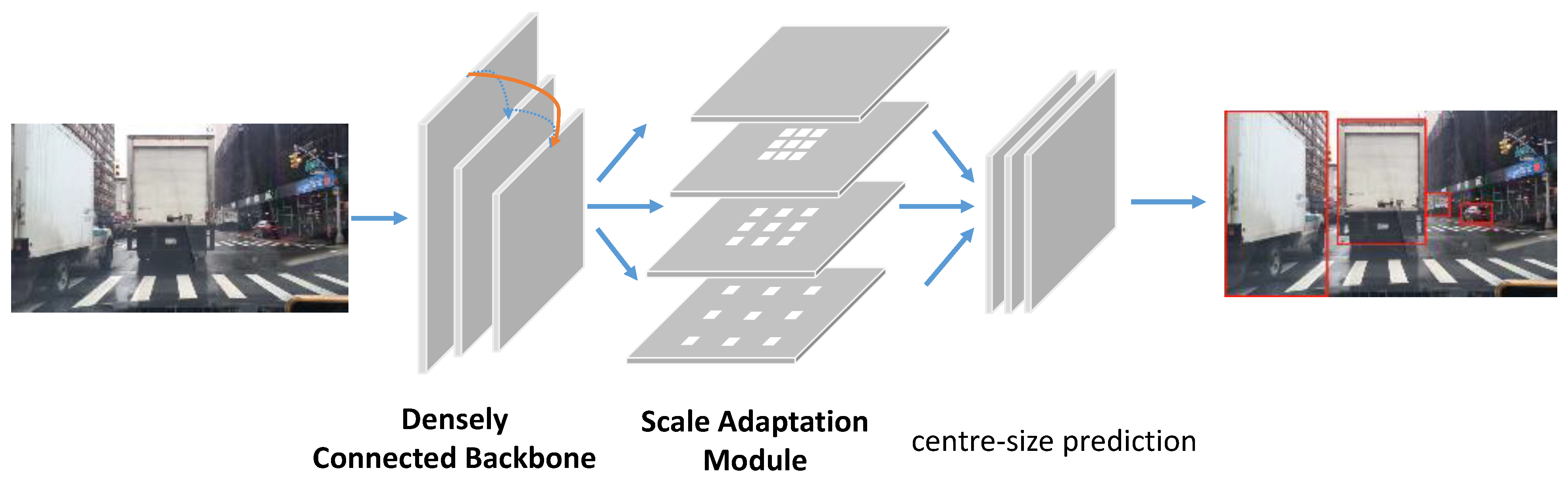
Inference Speed. In this work, to maintain as much of the computational efficiency of the model as possible, we adopted the following strategies. First, we chose HRNet as the basis for our network because it connects high-to-low resolution convolution streams in parallel. Second, we only added the skip connection between level 2 and level 4 feature maps, as shown in Figure 3, rather than connecting all low-level features to high-level features, such as DenseNet. Third, in our scale adaptation module, different branches are connected in parallel, which is different from the serial connection of YOLOF. We compared and verified the inference speed of the method; in particular, we compared the inference speed with different backbone features. As can be seen in

Table 9. The model’s inference speed on the KITTI dataset. The resolution of all the input images was set to be the same. All the models were tested on the same computing platform. The stack number of Hourglass was set to 1.

Method	Backbone	Millisecond/Image
ATSS	ResNet-101-FPN	39
CenterNet	Hourglass	29
	HRNet-w48	73
Ours (SA-CenterNet)	Hourglass	37
	HRNet-w48	91

, when adopting the same Hourglass backbone, the inference time of our method was only 8 ms longer than that of the baseline model, CenterNet. In addition, when adopting the HRNet-w48 backbone with high-resolution features, the inference time of our method was only 18 ms longer than that of CenterNet. Notably, our method was 2 ms faster than the state-of-the-art ATSS when using a slim Hourglass. These results show that our method does not significantly improve the inference time.

Model Stability. To test the stability of our model, we conducted multiple sets of experiments with different random seeds. We plotted the error–epoch curves on the test dataset of KITTI, as shown in Figure 5. The mean and standard deviation are approximately 0.45 and 0.01, respectively, when converged.

4.5. Qualitative Results

We provide a visualization of the results achieved by CenterNet and our approach on the KITTI dataset in Figure 6. The first column, the second column, and the third column are the visualization results of the original CenterNet, our method, and the ground truth, respectively. The three images in the first row show that our method successfully detected nearby large-scale pedestrians without false detections of trucks. The pictures in the second row indicate that our method successfully detected both the nearest and the farthest pedestrians. The images in the third row show that our method successfully detected nearby large-scale cyclists without false detection of pedestrians. The images in the fourth row show that our method successfully reduced the false detection of the farthest pedestrian. From the pictures in the last row, we can see that our method successfully detected nearby large-scale cyclists. These results demonstrate that our method achieves better detection performance for objects of different scales than CenterNet.

5. Conclusions

In this paper, aiming to address the insufficient adaptability of the classic anchor-free model lacking the FPN module to object scale variation, such as CenterNet, we propose a divide-and-conquer strategy and introduce some prior information about the object’s scale into the model. Based on CenterNet, we propose SA-CenterNet in this paper. Specifically, an improved high-resolution feature extraction network is proposed to adapt to small-scale object detection, and a scale adaptation module is designed to adapt to the detection of large-scale objects and object scale variation. Finally, a large number of experiments are performed on two publicly used road scene camera image object detection datasets for autonomous driving. The experimental results show that the proposed model outperforms the original, classic CenterNet and other recent anchor-free detectors with the FPN module in the detection of objects with different scales, and the effectiveness of each module of the model is verified by ablation experiments.

In the future, we intend to explore dynamic scale-adaptive networks and generalize our approach to different types of detectors, such as studying the scale adaptation problem based on the recently popular transformer-based detectors.

References

1. Wei, J.; He, J.; Zhou, Y.; Chen, K.; Tang, Z.; Xiong, Z. Enhanced object detection with deep convolutional neural networks for advanced driving assistance. IEEE Trans. Intell. Transp. Syst. 2019, 21, 1572–1583. [Google Scholar] [CrossRef] [Green Version]
2. Condat, R.; Rogozan, A.; Bensrhair, A. Gfd-retina: Gated fusion double retinanet for multimodal 2d road object detection. In Proceedings of the 2020 IEEE 23rd International Conference on Intelligent Transportation Systems (ITSC), Rhodes, Greece, 20–23 September 2020; pp. 1–6. [Google Scholar]
3. Bateni, S.; Wang, Z.; Zhu, Y.; Hu, Y.; Liu, C. Co-optimizing performance and memory footprint via integrated cpu/gpu memory management, an implementation on autonomous driving platform. In Proceedings of the 2020 IEEE Real-Time and Embedded Technology and Applications Symposium (RTAS), Sydney, NSW, Australia, 21–24 April 2020; pp. 310–323. [Google Scholar]
4. He, Y.; Wang, J. Deep mixture density network for probabilistic object detection. In Proceedings of the 2020 IEEE/RSJ International Conference on Intelligent Robots and Systems (IROS), Las Vegas, NV, USA, 24 October 2020–24 January 2021; pp. 10550–10555. [Google Scholar]
5. LeCun, Y.; Bengio, Y.; Hinton, G. Deep learning. Nature 2015, 521, 436–444. [Google Scholar] [CrossRef] [PubMed]
6. Liu, L.; Ouyang, W.; Wang, X.; Fieguth, P.; Chen, J.; Liu, X.; Pietikäinen, M. Deep learning for generic object detection: A survey. Int. J. Comput. Vis. 2020, 128, 261–318. [Google Scholar] [CrossRef] [Green Version]
7. Carranza-García, M.; Torres-Mateo, J.; Lara-Benítez, P.; García-Gutiérrez, J. On the performance of one-stage and two-stage object detectors in autonomous vehicles using camera data. Remote Sens. 2020, 13, 89. [Google Scholar] [CrossRef]
8. Girshick, R.; Donahue, J.; Darrell, T.; Malik, J. Rich feature hierarchies for accurate object detection and semantic segmentation. In Proceedings of the IEEE Conference on Computer Vision and Pattern Recognition, Columbus, OH, USA, 23–28 June 2014; pp. 580–587. [Google Scholar]
9. Girshick, R. Fast r-cnn. In Proceedings of the IEEE International Conference on Computer Vision, Santiago, Chile, 7–13 December 2015; pp. 1440–1448. [Google Scholar]
10. He, K.; Zhang, X.; Ren, S.; Sun, J. Spatial pyramid pooling in deep convolutional networks for visual recognition. IEEE Trans. Pattern Anal. Mach. Intell. 2015, 37, 1904–1916. [Google Scholar] [CrossRef] [PubMed] [Green Version]
11. Ren, S.; He, K.; Girshick, R.; Sun, J. Faster R-CNN: Towards real-time object detection with region proposal networks. IEEE Trans. Pattern Anal. Mach. Intell. 2016, 39, 1137–1149. [Google Scholar] [CrossRef] [PubMed] [Green Version]
12. Liu, W.; Anguelov, D.; Erhan, D.; Szegedy, C.; Reed, S.; Fu, C.Y.; Berg, A.C. Ssd: Single shot multibox detector. In Computer Vision—ECCV 2016. ECCV 2016; Springer: Cham, Switzerland, 2016; pp. 21–37. [Google Scholar]
13. Xu, X.; Zhao, J.; Li, Y.; Gao, H.; Wang, X. BANet: A Balanced Atrous Net Improved from SSD for Autonomous Driving in Smart Transportation. IEEE Sens. J. 2020, 21, 25018–25026. [Google Scholar] [CrossRef]
14. Qian, H.; Wu, P.; Sun, B.; Su, S. AGS-SSD: Attention-Guided Sampling for 3D Single-Stage Detector. Electronics 2022, 11, 2268. [Google Scholar] [CrossRef]
15. Redmon, J.; Divvala, S.; Girshick, R.; Farhadi, A. You only look once: Unified, real-time object detection. In Proceedings of the IEEE Conference on Computer Vision and Pattern Recognition, Las Vegas, NV, USA, 27–30 June 2016; pp. 779–788. [Google Scholar]
16. Redmon, J.; Farhadi, A. Yolov3: An incremental improvement. arXiv 2018, arXiv:1804.02767. [Google Scholar]
17. Law, H.; Deng, J. Cornernet: Detecting objects as paired keypoints. In Proceedings of the European Conference on Computer Vision (ECCV), Munich, Germany, 8–14 September 2018; pp. 734–750. [Google Scholar]
18. Tian, Z.; Shen, C.; Chen, H.; He, T. Fcos: Fully convolutional one-stage object detection. In Proceedings of the IEEE/CVF International Conference on Computer Vision, Seoul, Korea, 27 October–2 November 2019; pp. 9627–9636. [Google Scholar]
19. Zhou, X.; Wang, D.; Krähenbühl, P. Objects as points. arXiv 2019, arXiv:1904.07850. [Google Scholar]
20. Zhang, S.; Chi, C.; Yao, Y.; Lei, Z.; Li, S.Z. Bridging the gap between anchor-based and anchor-free detection via adaptive training sample selection. In Proceedings of the IEEE/CVF Conference on Computer Vision and Pattern Recognition, Seattle, WA, USA, 13–19 June 2020; pp. 9759–9768. [Google Scholar]
21. Lin, T.Y.; Dollár, P.; Girshick, R.; He, K.; Hariharan, B.; Belongie, S. Feature pyramid networks for object detection. In Proceedings of the IEEE Conference on Computer Vision and Pattern Recognition, Honolulu, HI, USA, 21–26 July 2017; pp. 2117–2125. [Google Scholar]
22. Geiger, A.; Lenz, P.; Urtasun, R. Are we ready for autonomous driving? The kitti vision benchmark suite. In Proceedings of the 2012 IEEE Conference on Computer Vision and Pattern Recognition, Providence, RI, USA, 16–21 June 2012; pp. 3354–3361. [Google Scholar]
23. Yu, F.; Chen, H.; Wang, X.; Xian, W.; Chen, Y.; Liu, F.; Madhavan, V.; Darrell, T. Bdd100k: A diverse driving dataset for heterogeneous multitask learning. In Proceedings of the IEEE/CVF Conference on Computer Vision and Pattern Recognition, Seattle, WA, USA, 13–19 June 2020; pp. 2636–2645. [Google Scholar]
24. Yu, F.; Koltun, V. Multi-scale context aggregation by dilated convolutions. arXiv 2015, arXiv:1511.07122. [Google Scholar]
25. Yin, X.; Liu, X. Multi-task convolutional neural network for pose-invariant face recognition. IEEE Trans. Image Process. 2017, 27, 964–975. [Google Scholar] [CrossRef] [PubMed] [Green Version]
26. Singh, B.; Davis, L.S. An analysis of scale invariance in object detection snip. In Proceedings of the IEEE Conference on Computer vision and Pattern Recognition, Salt Lake City, UT, USA, 18–22 June 2018; pp. 3578–3587. [Google Scholar]
27. Ghiasi, G.; Lin, T.Y.; Le, Q.V. Nas-fpn: Learning scalable feature pyramid architecture for object detection. In Proceedings of the IEEE/CVF Conference on Computer Vision and Pattern Recognition, Long Beach, CA, USA, 16–20 June 2019; pp. 7036–7045. [Google Scholar]
28. Wang, X.; Zhang, S.; Yu, Z.; Feng, L.; Zhang, W. Scale-equalizing pyramid convolution for object detection. In Proceedings of the IEEE/CVF Conference on Computer Vision and Pattern Recognition, Seattle, WA, USA, 13–19 June 2020; pp. 13359–13368. [Google Scholar]
29. Hwang, B.; Lee, S.; Han, H. LNFCOS: Efficient Object Detection through Deep Learning Based on LNblock. Electronics 2022, 11, 2783. [Google Scholar] [CrossRef]
30. Li, Y.; Chen, Y.; Wang, N.; Zhang, Z. Scale-aware trident networks for object detection. In Proceedings of the IEEE/CVF International Conference on Computer Vision, Seoul, Korea, 27 October–2 November 2019; pp. 6054–6063. [Google Scholar]
31. Pang, Y.; Zhao, X.; Zhang, L.; Lu, H. Multi-scale interactive network for salient object detection. In Proceedings of the IEEE/CVF Conference on Computer Vision and Pattern Recognition, Seattle, WA, USA, 13–19 June 2020; pp. 9413–9422. [Google Scholar]
32. Chen, Q.; Wang, Y.; Yang, T.; Zhang, X.; Cheng, J.; Sun, J. You only look one-level feature. In Proceedings of the IEEE/CVF Conference on Computer Vision and Pattern Recognition, Nashville, TN, USA, 20–25 June 2021; pp. 13039–13048. [Google Scholar]
33. Sun, K.; Xiao, B.; Liu, D.; Wang, J. Deep high-resolution representation learning for human pose estimation. In Proceedings of the IEEE/CVF Conference on Computer Vision and Pattern Recognition, Long Beach, CA, USA, 16–20 June 2019; pp. 5693–5703. [Google Scholar]
34. Huang, G.; Liu, S.; Van der Maaten, L.; Weinberger, K.Q. Condensenet: An efficient densenet using learned group convolutions. In Proceedings of the IEEE Conference on Computer Vision and Pattern Recognition, Salt Lake City, UT, USA, 18–22 June 2018; pp. 2752–2761. [Google Scholar]
35. Liu, S.; Qi, L.; Qin, H.; Shi, J.; Jia, J. Path aggregation network for instance segmentation. In Proceedings of the IEEE Conference on Computer Vision and Pattern Recognition, Salt Lake City, UT, USA, 18–22 June 2018; pp. 8759–8768. [Google Scholar]
36. Lin, T.Y.; Maire, M.; Belongie, S.; Hays, J.; Perona, P.; Ramanan, D.; Dollár, P.; Zitnick, C.L. Microsoft coco: Common objects in context. In Computer Vision—ECCV 2014; Springer: Cham, Switzerland, 2014; pp. 740–755. [Google Scholar]
37. Chen, K.; Wang, J.; Pang, J.; Cao, Y.; Xiong, Y.; Li, X.; Sun, S.; Feng, W.; Liu, Z.; Xu, J.; et al. MMDetection: Open MMLab Detection Toolbox and Benchmark. arXiv 2019, arXiv:1906.07155. [Google Scholar]
Figure 1. The distribution of the range of variation of the object scale on the KITTI and BDD100K datasets. The scale on the y-axis represents the maximum side length of the object’s bounding box. The x-axis represents the number of objects whose scale does not exceed the corresponding value of the y-axis. (a) KITTI. (b) BDD100K.
Electronics 11 03303 g001
Figure 2. The overall architecture of our SA-CenterNet, which primarily consists of a densely connected backbone, a scale adaptation module and a center-size prediction module. The first two modules are proposed in this paper and introduced in the text below. The center-size prediction module is the same as that in the original CenterNet.
Electronics 11 03303 g002
Figure 3. Simplified architectures of HRNet and the densely connected HRNet. The blue dotted line in the figure corresponds to the connecting line of the original HRNet. The solid red line in the figure represents the proposed short-circuit connection line to connect the initial high-resolution convolutional feature maps to the later low-resolution convolutional feature maps. (a) HRNet. (b) Densely Connected HRNet.
Electronics 11 03303 g003
Figure 4. (a) shows the architecture of the scale-aware module, and (b) shows the dilated convolution module in detail. In (a), Scale-aware-n represents a dilated convolution module with expansion rate n. Scale-aware-0 represents a direct connection to transmit the previous layer information more efficiently. In (b), Conv1 contains a convolution layer with a kernel size of 1 × 1 , a batch normalization layer, and a ReLU layer. Conv3 contains a convolution layer with a kernel size of 3 × 3 , a batch normalization layer and a ReLU layer. Conv-dilation-n contains a dilated convolution module with expansion rate n, a batch normalization layer, and a ReLU layer.
Electronics 11 03303 g004
Figure 5. The error–epoch curves on the test dataset from three rounds of experiments with different random seeds.
Electronics 11 03303 g005
Figure 6. Visualization of detection results on the KITTI dataset. The first column in the figure shows the detection results from the original CenterNet, the second column shows the detection results from SA-CenterNet, and the third column shows the ground truth. These results demonstrate that our method achieves better detection performance for objects of different scales. The object categories are Car, Van, Truck, Pedestrian, Person_sitting, Cyclist, Tram, Misc.
Electronics 11 03303 g006