IoT Anomaly Detection Based on Autoencoder and Bayesian Gaussian Mixture Model

Abstract

The Internet of Things (IoT) is increasingly providing industrial production objects to connect with the physical world and has been widely used in various fields. Although it has brought great industrial convenience, there are also potential security threats due to the vulnerabilities and malicious nodes in IoT. To correctly identify the traffic of malicious nodes in IoT and reduce the damage caused by malicious attacks on IoT devices, this paper proposes an autoencoder-based IoT malicious node detection method. The contributions of this paper are as follows: firstly, the high complexity multi-featured traffic data are processed and dimensionally reduced through the autoencoder to obtain the low-dimensional feature data. Then, the Bayesian Gaussian mixture model is adopted to cluster the data in a low-dimensional space to detect anomalies. Furthermore, the method of variational inference is used to estimate the parameters in the Bayesian Gaussian mixture model. To evaluate our model’s effectiveness, we used a public dataset for our experiments. As a result, in the experiment, the proposed method achieves a high accuracy rate of 99% distinguishing normal and abnormal traffic with three-dimension data reduced by the autoencoder, and it establishes our model’s better detection performance compared with previous K-means and Gaussian Mixture Model (GMM) solutions.

1. Introduction

Industry 4.0 has brought the Internet of Things (IoT) into every industrial development field, which has positively impacted industrial development [1]. Industrial IoT is a subset of IoT, and IoT technology plays a crucial role in modern industry by introducing automation and incorporating IoT sensors into industrial systems [2]. According to Accenture, the Industrial IoT will be worth USD 7.1 trillion for the United States and more than USD 1.2 trillion for Europe by 2030 [3].

Although the Internet of Things offers many opportunities for industrial development, it also faces a growing number of problems. Due to the complexity of IoT devices, their vulnerability to attacks is greatly increased. Many potential security issues, such as vulnerabilities and mobile threats, will significantly affect the security and privacy reliability of IoT [4]. Some miscreants use IoT vulnerabilities— which are caused by a variety of constraints, such as limited resources and weak IoT security [5]—to access legitimate devices, such as using malicious packet injection and distributed denial of service (DDoS) attacks. Almost half of the US was plunged into disconnection by a DDoS attack on US service provider Dyn in October 2016 [6]. This massive DDoS attack was launched by IoT devices infected with the Mirai virus. In early 2020, the FDA identified a vulnerability in St. Jude Medical implantable cardiac devices that occurred in transmitters that read device data and share it remotely with physicians, allowing hackers to control appliances by accessing their transmitters, including pacemakers and defibrillators, and an attack would pose a serious threat to patient lives [7]. It follows that an attack on the IoT would be a huge loss, and without security, the IoT would not be able to reach its full potential in the industry.

A primary key to solving security problems in IoT lies in discovering abnormal nodes in the network. In practical applications of IoT, abnormal behavior of nodes may come from network attacks, or nodes may be in an abnormal state due to environmental factors, failures, etc. We classify anomalies in IoT into two categories: interventional anomalies and non-interventional anomalies; interventional anomalies are also anomalies caused by network attacks in the usual sense, such as DDoS attacks, replay attacks, etc., whereas non-interventional anomalies are those caused by device failures. Noninterventional anomalies are easy to find, while interventional anomalies need to be detected by detection means; thus, this paper takes interventional anomalies as the primary research object.

Cyberattacks generally cause network traffic not to conform to the expected behavior pattern [8]. To alleviate network attacks, mitigate the damage caused by intervening anomalies in the IoT environment, and further improve the efficiency and security of the IoT, researchers have introduced anomaly detection to identify behaviors that compromise the security of the IoT, and this detection usually utilizes the unintended behavior patterns caused by network attacks for anomaly identification. There are various methods for intervening to detect anomalies in the IoT, mainly statistical-based methods, feature selection-based methods, and machine learning-based methods.

Network traffic data are usually untagged; therefore, unsupervised anomaly detection methods are traditionally used to distinguish normal and abnormal traffic data in the IoT. Unsupervised anomaly detection deals with traffic data that are manually extracted from complex network systems, which are generally characterized by high dimensionality, strong redundancy, and low correlation. It is challenging to perform anomaly detection on unsupervised high-dimensional data. Since it is difficult to have a more intuitive understanding of high-dimensional data, the higher the dimensionality of the data, the more difficult it is to perform anomaly detection tasks in the original dimensional space. On the basis of the current development status of IoT anomaly detection, we summarize the existing problems of anomaly detection as follows:

• Higher dimensionality of data, which is more complex to process;
• A certain degree of randomness and uncertainty in the selection of features using feature selection methods;
• Clustering algorithms are often used to classify normal and abnormal data. However, traditional clustering algorithms, such as K-means, need to manually specify clusters and have certain limitations. Their clustering results are easily disturbed by noise points and easily fall into local optima.

In response to the above existing problems in anomaly detection, this paper proposes a Bayesian Gaussian mixture model based on autoencoder. The model uses an autoencoder to reduce high-dimensional data to low-dimensional data to achieve feature selection of the data; the Bayesian Gaussian mixture model is used to cluster low-dimensional data to achieve anomaly detection. The Bayesian Gaussian mixture model adopts the method of variational inference, uses posterior probability for parameter estimation, and dynamically adjusts the division of cluster classes, which solves the problem of the local optimum of the model. The contributions of this paper are as follows:

• We use an autoencoder for feature selection, which effectively solves the problem that high-dimensional data is difficult to handle, and the autoencoder feature selection method improves the uncertainty and randomness of other feature selection methods.
• We propose a Bayesian Gaussian mixture model based on autoencoder, which uses posterior probability for parameter estimation and dynamically adjusts the cluster class division to solve the problem that the model tends to fall into local optima; and the Bayesian Gaussian mixture model is useful for both the data class imbalance problem and the data complex hard-to-fit problem.
• We compare different methods used for anomaly detection, and the results show that the autoencoder-based Bayesian Gaussian mixture model achieves over 99% accuracy for anomaly detection.

We outline the framework of this article as follows. Section II summarizes the current research results related to IoT security. Section III describes the overall architecture and principles of the autoencoder-based Bayesian Gaussian mixture model. Section IV contains the experimental evaluation and provides an intuitive display of our experimental results. Section V summarizes our paper and concludes.

2. Related Work

Currently, a series of investigations have been carried out on anomaly detection in the IoT.

Firstly, the reconstruction-based method assumes that the samples of the target class are sufficiently clustered. Samples deviating from the model are judged as outliers through the model estimation and its parameters, such as the mean point, plane, surface or manifold, subspace, etc. [9]. Traditional methods in this category include principal component analysis (PCA) with explicit linear projections [10], kernel PCA (KPCA) with implicit nonlinear predictions induced by a specific kernel [11], and robust PCA (RPCA) that makes PCA less sensitive to noise by enforcing sparse structure [12]. However, the performance of the reconstruction-based anomaly detection method is limited. This method can only detect anomalies on the part of the reconstruction error. Although the compression and model estimation of abnormal samples and normal samples may be very different, and some abnormal samples have high reconstruction errors when the samples have considerable noise, there are still a large number of abnormal samples whose reconstruction errors are close to those of normal samples.

Secondly, cluster analysis is a popular anomaly detection method which groups objects with similar features into a group in an unsupervised way, such as a multivariate Gaussian model, Gaussian mixture model, K-means, etc. In the literature [13], Chang et al. adopted two anomaly detection algorithms, K-means algorithm and convolution auto-encoding algorithm, to perform anomaly detection. The K-means anomaly detection module aims to detect whether each attribute value is within the normal range. In principle, all attributes are used as far as possible, but if there is no influence between attributes, they will be filtered out. The task of the convolution autoencoder anomaly detection module is to learn the normal change pattern of multiple attributes in continuous time. Finally, the two modules are formed into a double anomaly detection module. Only when the predicted outputs of the two modules are normal will the test data be predicted to be normal. However, this method does not use a proprietary feature selection algorithm in feature selection, and only manually filters out the attributes that have no impact, which is very random. In the literature [9], Bozong et al. proposed a deep autoencoding Gaussian mixture model (DAGMM) which uses a deep autoencoder to store the critical information of a sample in a low-dimensional space, and the DAGMM uses a Gaussian mixture model (GMM) in the learned low-dimensional space to handle the density estimation task for input data with complex structures. However, Gaussian mixture models (GMM) are usually learned by alternate algorithms such as expectation maximization algorithms (EM), which can easily lead to local optima and do not perform well for anomaly detection.

Deep learning methods are also more common in anomaly detection, such as convolutional neural network (CNN) [14,15], recurrent neural network (RNN) [16,17,18], generative adversarial neural network (GAN) [19,20,21], and long short-term memory neural network (LSTM) [22], etc. Ferrag et al. [15] studied CNN, RNN, and deep neural network (DNN) for intrusion detection and their performance in different approaches. The performance of CNN was compared and analyzed under different configurations. Still, CNN has a drawback that makes it impossible to ignore, i.e., they cannot learn the long-time dependent features of IoT traffic. The literature [23] proposes a compressed convolutional variational autoencoder for anomaly detection of time-series data in IIoT, which reduces the model’s size and inference time, but the classification performance is largely unimproved; additionally in the literature [24], Sumathi et al. propose a DDoS attack detection mechanism using neural networks. Their model uses a deep learning classifier based on a publicly available data-integration cost-minimization strategy to evaluate network traffic. Detection accuracy, sample cost, packet loss rate, average delay, packet delivery rate, overhead, and throughput are used as evaluation metrics for performance analysis. However, the algorithm suffers from computational overload when used on IoT data with a large number of features and a large data volume, which will reduce the efficiency of anomaly detection.

In addition, one-classification methods (one-class) are also widely used for anomaly detection, which learn discriminative boundaries around normal data by algorithms. For example, the one-classification support vector machine (OCSVM) learns the boundary of normal data and identifies all events or data points outside the boundary as abnormal behavior of the system [25]. However, when the number of dimensions increases, the performance of this method is usually unsatisfactory due to the high dimensionality of the data.

The Bayesian Gaussian mixture model based on autoencoder proposed in this paper performs anomaly detection in the low-dimensional feature space learned by the autoencoder, which well avoids the problem that high-dimensional data are difficult to handle, and at the same time, it reduces the computational effort and improves the computational efficiency. In addition, the Bayesian Gaussian mixture model adaptively acquires hyperparameters during the model construction process and has a clear probabilistic interpretation of the output prediction.

3. Bayesian Gaussian Mixture Model Based on Autoencoder

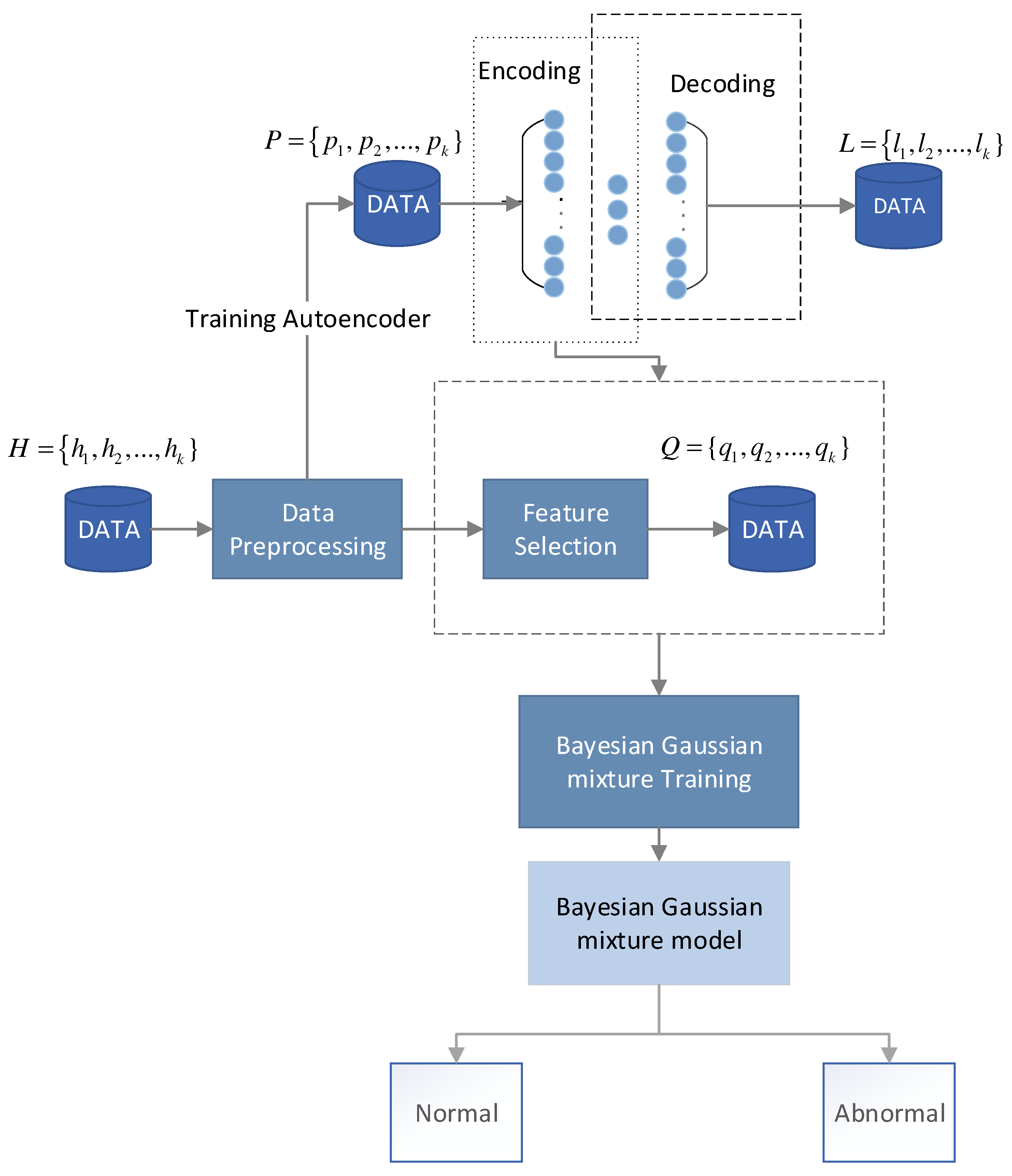
3.1. Methodology Model Overview

The method proposed in this paper is shown in Figure 1. Specifically, the first step of the model is to preprocess the original network traffic data $H=\left\{h_1,h_2,\dots ,h_k\right\}$. The original data have $k$ network traffic features, where $h_i={\left[f_1^i,f_2^i,\dots ,f_m^i\right]}^T$ denotes the $i$th $m$-dimensional ($m$ is 43 in this paper) network traffic feature vector, $i=1,2,\dots ,k$, pre-processed to obtain data $P=\left\{p_1,p_2,\dots ,p_k\right\}$.

The second step is to train the autoencoder model using the pre-processed data $P$, extract the encoder part, use the encoder part to dimensionalize the existing data, reduce the $m$-dimension data to $n$ dimensions ($m$ is much larger than $n$), and obtain the data $Q=\left\{q_1,q_2,\dots ,q_k\right\}$, where $q_i={\left[t_1^i,t_2^i,\dots ,t_n^i\right]}^T$ denotes the $j$th $n$-dimensional network traffic characteristic data after dimension processing, $i=1,2,\dots ,k$. The decoder reconstructs the data $L=\left\{l_1,l_2,\dots ,l_k\right\}$ and calculates the reconstruction errors of $P$ and $L$ to judge the merits of the autoencoder.

Finally, the low-dimensional data $Q$ is transmitted to the Bayesian Gaussian mixture model to obtain the weight of the cluster class and classify the data to determine whether the data is normal or abnormal.

3.2. Data Preprocessing

There are large magnitude differences between different features of the original network data, and if the data are directly applied to the Bayesian Gaussian mixture model of the autoencoder, it will increase computational effort and reduce computational accuracy. Therefore, it is necessary to normalize the data. The data normalization process converts all data into numbers between [0,1], and its purpose is to cancel the difference in magnitude between the data of each dimension so as to avoid the large error in network prediction due to the large difference in magnitude of the input and output data. In this paper, the Min-Max normalization method is used, and its calculation formula is as follows [26]:

$$p_j^i=\frac{f_j^i-\underset{1<j<m}{\min }\left\{f_j^i\right\}}{\underset{1<j<m}{\max }\left\{f_j^i\right\}-\underset{1<j<m}{\min }\left\{f_j^i\right\}},$$

(1)

where $\underset{1<j<m}{\min }\left\{f_j^i\right\}$ is the minimum value of the original attribute and $\underset{1<j<m}{\max }\left\{f_j^i\right\}$ is the maximum value of the original attribute.

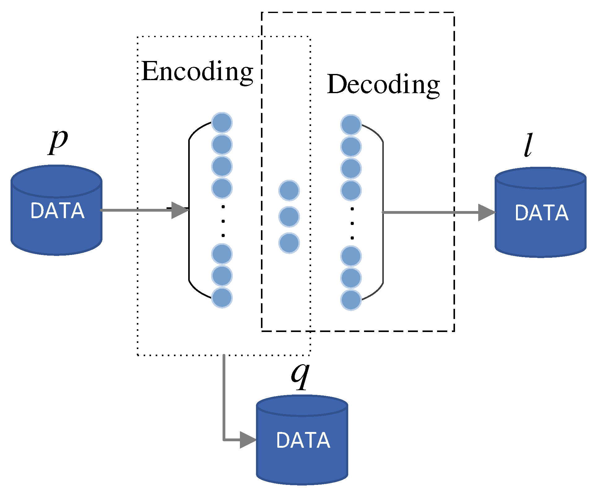
3.3. Autoencoder Network-Based Feature Processing

The autoencoder is an unsupervised deep learning network model that reconstructs input data through the network for effective coding [27], which is usually used for feature learning and feature dimension reduction. The structure of the autoencoder is shown in Figure 2. The autoencoder compresses the original data features by the encoder to get new features and then reconstructs the original data by the decoder.

In this paper, the autoencoder neural network is used to process data features. Given a sample $P$, its learning process through the autoencoder is as follows:

$$q=g_1(p,{\theta }_e),$$

(2)

$$l=g_2(q,{\theta }_d),$$

(3)

$$L(p,l)={‖p-l‖}^2,$$

(4)

where $q$ is the low-dimensional representation learned by the autoencoder, ${\theta }_e$ and ${\theta }_d$ are the parameters of the encoding part and decoding part, respectively, $g_1\left(.\right)$ denotes the encoding function, $g_2\left(.\right)$ denotes the decoding function, and $L\left(p,l\right)$ is the loss function characterizing the reconstruction error of the autoencoder.

The internal network structure of the autoencoder is presented in Figure 3. The encoding part and the decoding part are two fully connected layers, where Dense1 is the fully connected layer for the encoding part, and Dense2 is the fully connected layer for the decoding part.

3.4. Bayesian Gaussian Mixture Model

After learning the low-dimensional representation q of the data through the autoencoder, anomaly detection is performed in the framework of a Bayesian Gaussian mixture model.

Gaussian mixture models quantify the exact representation of observations by means of Gaussian probability densities. Each Gaussian mixture model consists of $K$ Gaussian distributions, then each observation q has the following distribution [28]:

$$P(q_i|\pi ,\mu ,\gamma )={\displaystyle \sum _{j=1}^K{\pi }_{j}N(q_i|{\mu }_j,{\gamma }_j^{-1})},$$

(5)

where the observation $q_i$ is the low-dimensional data obtained by the autoencoder, $\mu =\left\{{\mu }_j\right\}$ is the mean, $\gamma =\left\{{\gamma }_j\right\}$ is the covariance matrix, $\pi =\left\{{\pi }_j\right\}$ is the mixing coefficient, and ${\displaystyle \sum _{j=1}^K{\pi }_j=1}$, then the observation can be obtained by the following process:

$$c_i~categorical({\pi }_1,{\pi }_2,\dots ,{\pi }_K),$$

(6)

$$p_i|c_i~\mathrm{N}({\mu }_{c_i},{\gamma }_{c_i}^{-1}),$$

(7)

In this paper, we expand the simple Gaussian mixture model into a full Bayesian model, and use the mixture coefficient, mean value, and covariance matrix as latent variables in the prior distribution.

$$P({\pi }_1,{\pi }_2,\dots ,{\pi }_K|{\alpha }_0)=\frac{\Gamma (K{\alpha }_0)}{{\left[\Gamma ({\alpha }_0)\right]}^K}{\pi }_1^{{\alpha }_0-1}\dots {\pi }_K^{{\alpha }_0-1},$$

(8)

where ${\alpha }_0$ is the concentration parameter, the larger its value, the more likely the value of the mixing coefficient is to be close to zero, and $\Gamma (x)$ is Gamma function. Using the normal–Wishart distribution as the conjugate prior for the multivariate normal likelihood, the mean and covariance matrices are sampled,

$$P({\mu }_j,{\gamma }_j)=\mathrm{N}({\mu }_j|{\beta }_0{({\eta }_0{\gamma }_j)}^{-1})W({\gamma }_j|{\upsilon }_0,{\sigma }_0),$$

(9)

Therefore, the process of generation of the Bayesian Gaussian mixture model for each observation is as follows:

$${\pi }_1,\dots ,{\pi }_K~Dir({\alpha }_0),$$

(10)

$$c_i~categorical({\pi }_1,\dots ,{\pi }_K),$$

(11)

$$({\mu }_j,{\gamma }_j)~NW({\beta }_0,{\eta }_0,{\upsilon }_0,{\sigma }_0),$$

(12)

$$p_i|c_i~\mathrm{N}({\mu }_{c_i},{\gamma }_{c_i}^{-1}),$$

(13)

The traditional Gaussian mixture model uses the EM algorithm to iteratively solve the parameters, but the EM algorithm does not always find the optimal global solution in practice, and it must specify the number of clusters [29]. Obviously, for interventional anomaly detection, this approach is not applicable because the total number of attack types is not known before detection; therefore, the method of variational inference is chosen to solve the parameters.

Variational inference plays a good role in solving the posterior probabilities of observations and latent variables. In general, the calculation of posterior probabilities of observations and latent variables is complicated, and this problem is solved using the method of variational inference to obtain an approximation of the posterior probability instead of the true value, which, in turn, infers to which cluster the observation most likely belongs [30]. Suppose the variational distribution is $q(\pi ,c,\mu ,\gamma )$, which can be decomposed as:

$$q(\pi ,c,\mu ,\gamma )=q(\pi ){\displaystyle \prod _i^{m}q(c_i){\displaystyle \prod _{j=1}^{k}q({\mu }_j,{\gamma }_j)}},$$

(14)

From the variational inference, we can obtain the variational distribution of each potential variable [31]:

$$q^{*}(c_i)=categorical(c_i|{\varphi }_{i1},\dots ,{\varphi }_{ik}),$$

(15)

$$q^{*}(\pi )=Dirichlet(\pi |{\alpha }_1,\dots ,{\alpha }_k),$$

(16)

$$q^{*}({\mu }_j,{\gamma }_j)=N({\mu }_j|{\beta }_j,{({\eta }_j,{\gamma }_j)}^{-1})W({\gamma }_j|{\upsilon }_j,{\sigma }_j),$$

(17)

The variance distribution of the observation $q_i$ is a categorical distribution related to the parameter ${\varphi }_{i1},\dots ,{\varphi }_{ik}$, where ${\varphi }_{i1},\dots ,{\varphi }_{ik}$ can be obtained from the following equation:

$$\begin{array}{l}\ln {\varphi }_{ij}=(\psi ({\alpha }_j)-\psi ({\displaystyle \sum _{t=1}^k{\alpha }_t}))+\\ \frac{1}{2}({\displaystyle \sum _{t=1}^D(\frac{{\sigma }_j+1-t}{2})+D}\ln 2+\ln |{\nu }_j|)+\\ (-\frac{D}{2{\eta }_j}-\frac{{\sigma }_j}{2}(q_i-{\beta }_j){\nu }_j(q_i-{\beta }_j{)}^T)+const\end{array}$$

(18)

The variational distribution $q^{*}(\pi )$ is a Dirichlet function with parameters ${\alpha }_1,\dots ,{\alpha }_k$, where

$${\alpha }_j={\alpha }_0+N_j,$$

(19)

The variance distribution $q^{*}({\mu }_j,{\gamma }_j)$ is a normal–Wishart distribution containing four parameters, which are updated to the values:

$${\eta }_j={\eta }_0+N_j,$$

(20)

$${\beta }_j=\frac{1}{{\eta }_j}({\eta }_0{\beta }_0+N_j\overline{q_j}),$$

(21)

$${\nu }_j={\nu }_0^{-1}+N_j{S}_j+\frac{{\eta }_0{N}_j}{{\eta }_0+N_j}({\overline{q}}_j-{\beta }_0){({\overline{q}}_j-{\beta }_0)}^T,$$

(22)

$${\sigma }_j={\sigma }_0+N_j,$$

(23)

where

$$N_j={\displaystyle \sum _{i=1}^m{\varphi }_{ij}},$$

(24)

$${\overline{q}}_j=\frac{1}{N_j}{\displaystyle \sum _{i=1}^m{\varphi }_{ik}{q}_i},$$

(25)

$$S_j=\frac{1}{N_j}{\displaystyle \sum _{i=1}^m{\varphi }_{ij}(q_i-{\overline{q}}_j)}{\left(q_i-{\overline{q}}_j\right)}^T,$$

(26)

From this, we can find the approximate posterior distribution of $\pi ,c,\mu ,\gamma$. By iterating several times, we can obtain the most likely cluster of each observation $q_i$, and then implement the anomaly detection function.

4. Experiment and Analysis

4.1. Dataset Introduction

The data chosen for this article come from a publicly available dataset [32] whose authors created various types of attacks in an experimental setting, and whose raw packet files (in pcap format) were captured using the monitoring mode of a wireless network adapter.

This dataset main involves four attack methods: MITM, DoS, Scanner, and Mirai. In this paper, packets obtained by two types of attack methods, MITM attack and Mirai virus, are selected for analysis. MITM attacks (Man-In-The-Middle) mainly connect target devices and routes through ARP spoofing or DNS spoofing to eavesdrop and control the transmission of information, causing information leakage [33]. The Mirai virus is a type of virus that searches for IoT devices through the Internet. Once it scans an IoT device (e.g., webcam, smart switch, etc.), it tries to log in using the default or weak password, and once the login is successful, this IoT device starts to be manipulated by hackers to attack other network devices. With the exception of the Mirai botnet category, all of the attack data are packets captured during simulated attacks using tools such as Nmap.

In order to verify the validity of the model in this paper, labeled data were used to validate the model in this paper. After preliminary processing, we divided the data into six categories and used the feature selection method of the literature [33] to roughly select the features on the data to obtain data with 43-dimensional features.

Table 1. Flow types and their classification.

Flow Types	Description
benign	Data
arpspoofing	Traffic data of MITM (arp spoofing)
udpflooding	UDP attack traffic data from bot computers compromised by Mirai malware
udpflooding	ACK attack traffic data for bot computers compromised by Mirai malware
httpflooding	HTTP Flooding attack traffic data for bot computers compromised by Mirai malware
hostbrute	Initial stages of Mirai malware, including host discovery and Telnet exhaustive method

describes the traffic types and traffic sources of the six categories of data, which are benign, arpspoofing, udpflooding, ackflooding, httpflooding, and hostbrute, obtained from the attacks launched by MITM and Mirai.

Table 2. Selected characteristic index.

Index	Feature Name	Index	Feature Name
1	frame.time_epoch	23	tcp.flags
2	frame.time_delta	24	tcp.flags.ack
3	frame.time_delta_displayed	25	tcp.flags.push
4	frame.time_relative	26	tcp.flags.reset
5	frame.number	27	tcp.flags.syn
6	frame.len	28	tcp.window_size
7	frame.cap_len	29	tcp.window_size_scalefactor
8	eth.lg	30	tcp.checksum.status
9	ip.version	31	tcp.analysis.bytes_in_flight
10	ip.hdr_len	32	tcp.analysis.push_bytes_sent
11	ip.len	33	tcp.time_relative
12	ip.flags	34	icmp.ident
13	ip.flags.df	35	icmp.seq
14	ip.ttl	36	icmp.seq_le
15	ip.proto	37	data.len
16	ip.checksum.status	38	udp.srcport
17	tcp.stream	39	udp.dstport
18	tcp.len	40	udp.length
19	tcp.seq	41	udp.checksum.status
20	tcp.nxtseq	42	udp.stream
21	tcp.ack	43	dns.count.queries
22	tcp.hdr_len

shows the 43-dimensional features selected.

4.2. Feature Processing Using Autoencoder

In this paper, we build a three-layer neural network on TensorFlow framework to implement the function of autoencoder, the number of neurons in the input layer is 43. In Dense1, the number of input neurons is 43 and the number of output neurons is 3; in Dense2, the number of input neurons is set to 3 and the number of output neurons is set to 43. The Relu function is used as the activation function for the encoding part, the activation function used for the decoding part is the sigmoid function, and the mean square error is chosen to represent the loss function of the reconstruction error. The entire autoencoder is trained using the dataset, the model is trained using the Adam optimization algorithm, and finally the low-dimensional representation $q$ of the data learned by the encoder is used as the input data for the Bayesian Gaussian mixture model. When training the autoencoder, the learning rate LR is set to 0.001, the epoch is set to 15, and the batch size is set to 500.

Table 3. Flow types and their classifications.

Hyperparameter	Content
LR	0.001
Epoch	15
Batch size	500
Loss function	mse
Optimization algorithm	Adam
Activation function (Encoding)	Relu
Activation function (Decoding)	Sigmoid

summarizes the hyperparameter settings for the autoencoder network. Here, the activation function (Encoding) represents the activation function of the encoding part, and the activation function (Decoding) represents the activation function of the decoding part.

The variation in loss rate and accuracy during autoencoder training is demonstrated in Figure 4. The loss rate of the autoencoder starts to decrease at the 1st epoch and gradually converges to below 0.02 at the 6th epoch. The accuracy improves rapidly at the first epoch, with minor fluctuations between the 3rd and 11th epochs, and gradually stabilizes at the 12th epoch, with the accuracy finally converging to 0.90.

4.3. Cluster Analysis

4.3.1. Evaluation Indicators

In order to ensure the fairness of clustering performance evaluation, in this paper four widely used clustering model performance evaluation indices are used: Purity of clustering (P), Rand Index (RI), Adjusted Rand Index (ARI), and F-score, and the meanings represented by each index are described in detail below:

1.

P. Purity P is the most intuitive criterion to show how good the evaluation results are. Its calculation formula is as follows:

$$P=\left(\Omega ,C\right)=\frac{1}{N}{\displaystyle \sum _k{\max }_j\left|{\omega }_k\cap c_j\right|},$$

(27)

where $N$ denotes the total number of samples; $\Omega =\{{\omega }_1,{\omega }_2,\dots ,{\omega }_k\}$ denotes a cluster after clustering; $C=\{c_1,c_2,\dots ,c_j\}$ denotes the correct category; ${\omega }_k$ denotes all samples in the $k$th cluster after clustering; and $c_j$ denotes the number of true samples in the $j$th category after clustering. The value of P is in the range of [0,1], and the larger the value, the better the clustering effect.

2.

RI. The Rand Index (RI) is a common criterion for evaluating the effect of clustering and is calculated as follows:

$$RI=\frac{a+d}{a+b+c+d},$$

(28)

where $a$ denotes the number of data point pairs that group similar samples into the same cluster, $b$ is the number of data point pairs that group different samples into the same cluster, $c$ is the number of data point pairs that group similar samples into different clusters, and $d$ denotes the number of data point pairs that group dissimilar samples into different clusters. The value of the RI is between [0, 1], and the RI is 1 when the clustering results are perfectly matched.

3.

F-score. Similar to the F1 score in the classification index, it is calculated as follows:

$$\begin{array}{l}\mathrm{Pr}ecision=\frac{a}{a+b}\\ \mathrm{Re}call=\frac{a}{a+d}\\ F=(1+{\beta }^2)\frac{\mathrm{Pr}ecision·\mathrm{Re}call}{{\beta }^2·\mathrm{Pr}ecision+\mathrm{Re}call}\end{array}$$

(29)

where $\beta$ is a parameter, and in this paper, we set $\beta =1$.

4.

ARI. Adjusted Rand Index (ARI) is an improved version of the Rand Index (RI) to remove the influence of random labels on the RI assessment criteria. The API takes values in the range [−1,1], with larger values representing better results.

$$ARI=\frac{RI-E[RI]}{\max (RI)-E(RI)},$$

(30)

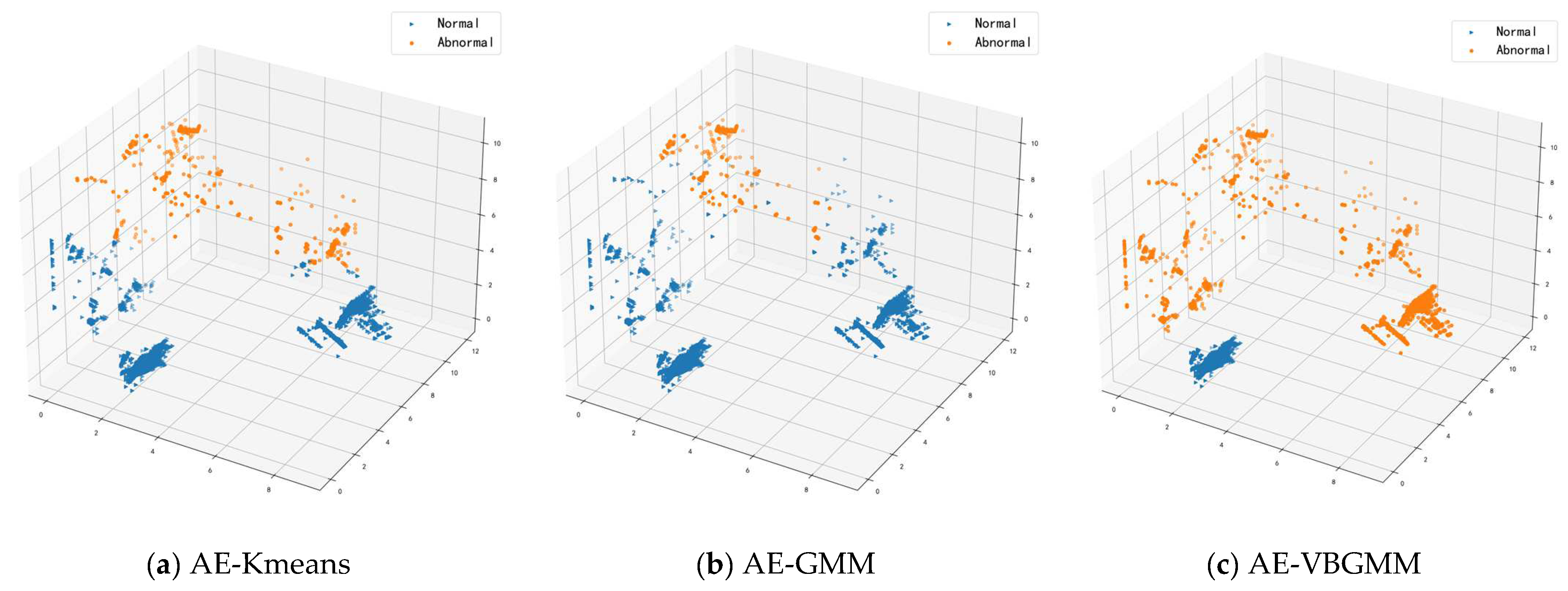
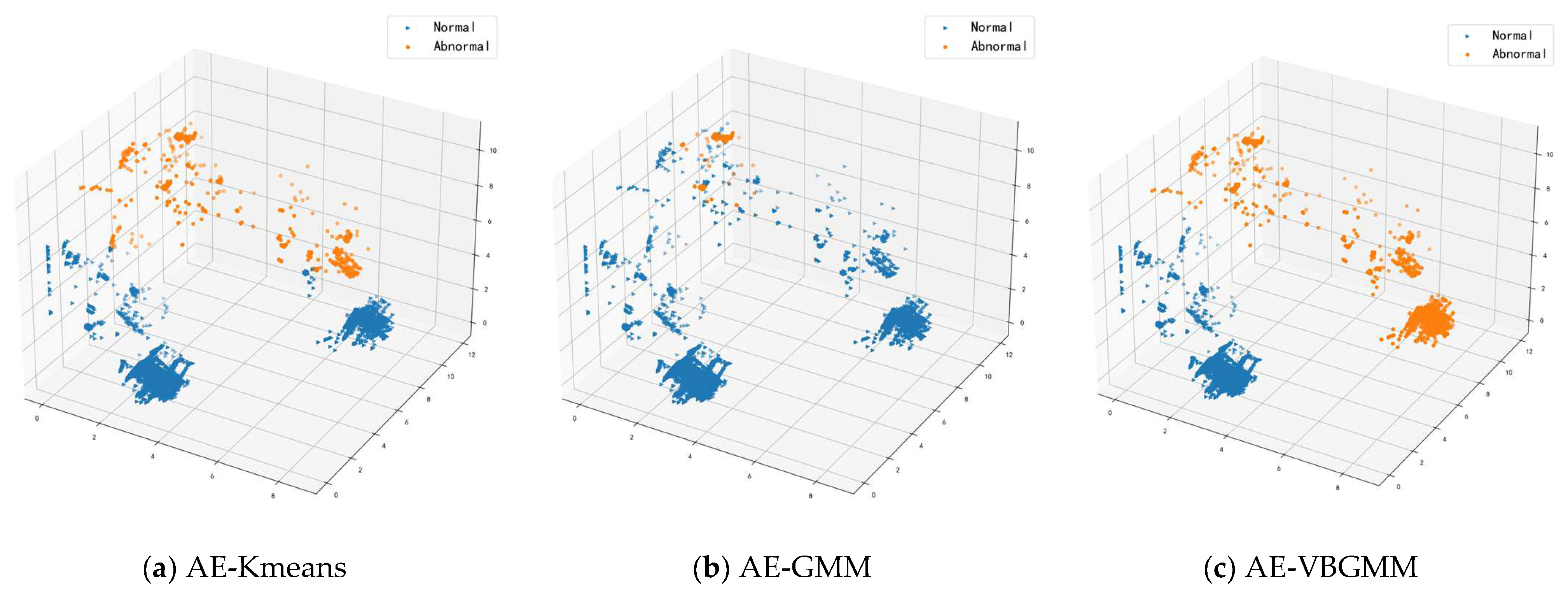
4.3.2. Analysis of Clustering Results

In this paper, we implement the anomaly detection method of the literature [9,13] and compare it with our proposed autoencoder Bayesian Gaussian mixture model.

• Autoencoder K-means model (AE-Kmeans). Refer to Section 4.2 for the parameter setting of the autoencoder; cluster class of K-means is set to 2.
• Autoencoder Gaussian Mixture Model (AE-GMM). The autoencoder parameter settings are referred to in Section 4.2, the number of cluster classes is set to 2 for GMM, and the number of iterations is set to 10.
• Bayesian Gaussian Mixture Model for Autoencoder (AE-VBGMM). The parameter setting of the autoencoder is described in Section 4.2. VBGMM sets the initial cluster class to 2, calculates the weight of each cluster, dynamically adjusts the number of cluster classes according to the weight, and sets the number of iterations to 10.

In the same dataset, two models, AE-Kmeans and AE-GMM, are implemented in this paper, and the results are visually represented and compared with AE-VBGMM.

The normal data benign were, respectively, combined with five different types of abnormal data for anomaly detection.

Table 4. P, RI, ARI, and F-score of AE-GMM with AE-VBGMM and AE-Kmeans with AE-VBGMM for anomaly detection. The best value of each evaluation criterion is marked in bold.

Attack	AE-GMM				AE-Kmeans				AE-VBGMM
	P	RI	ARI	F	P	RI	ARI	F	P	RI	ARI	F
hostbrute	1.000	1.000	1.000	1.000	0.999	0.998	0.997	0.998	1.000	1.000	1.000	1.000
ackflooding	0.885	0.797	0.579	0.833	0.887	0.799	0.585	0.834	0.995	0.991	0.981	0.991
arpspoofing	1.000	1.000	1.000	1.000	1.000	1.000	1.000	1.000	1.000	1.000	1.000	1.000
httpflooding	0.896	0.814	0.616	0.845	0.896	0.814	0.615	0.845	1.000	1.000	1.000	1.000
udpflooding	0.899	0.821	0.630	0.850	0.901	0.820	0.630	0.850	0.999	0.999	0.999	0.999

shows the values of P, RI, ARI, and F obtained after the three methods were used for anomaly detection. Three comparison experiments of AE-Kmeans, AE-GMM, and AE-VBGMM were performed using an autoencoder to reduce the dimensionality of the data and combining the three clustering methods of K-means, GMM, and VBGMM, respectively. When comparing the experimental results, it can be found that for the arpspoofing type of attack, all three methods can achieve a good clustering effect. For the attack type hostbrute, two methods, AE-GMM and AE-VBGMM, have sound cluster effects. For the other three attack types, the autoencoder Bayesian Gaussian mixture model proposed in this paper for anomaly detection is significantly better than the other two methods, with a clustering purity of more than 99% and little difference between K-means and GMM clustering effects. The poor clustering effect of K-means and GMM is because the clustering effect of K-means is closely related to the selection of the initial value, which is random. At the same time, the GMM uses the EM algorithm for parameter estimation, which is prone to fall into local optima.

Therefore, in this paper, the results of three attack types—other than arpspoofing and hostbrute—using three clustering algorithms, AE-Kmeans, AE-GMM, and AE-VBGMM, are visualized and displayed as follows with ARI as the main evaluation index.

The visualization results of anomaly detection by AE-Kmeans, AE-GMM, and AE-VBGMM for normal data benign and abnormal data ackflooding are shown in Figure 5. From the visualization results in the figure, we can see that AE-VBGMM can well separate normal data from abnormal data, and there is no overlap between them. In contrast, the results obtained by the two methods, AE-GMM and AE-Kmeans, have overlapping situations. There are 100,000 normal and 50,000 abnormal data in the experimental data, and the ratio of normal data to abnormal data is 2:1. Figure 5a indicates the results of the visualization of AE-Kmeans, which yielded 116,849 normal data and 33,151 abnormal data, where orange represents normal data, and blue represents abnormal data, with an ARI of 0.585. Figure 5b indicates the AE-GMM visualization results with 117,183 normal data and 32,817 abnormal data after clustering, with an ARI of 0.579. Figure 5c displays the visualization, results of the AE-VBGMM, with 100,057 normal data and 49,943 abnormal data after clustering and an ARI of 0.981. Obviously, for the attack type of ackflooding, the clustering effect of AE-VBGMM is better than those of AE-Kmeans and AE-GMM.

Figure 6 shows the anomaly detection visualization results of AE-Kmeans, AE-GMM, and AE-VBGMM that implement normal data benign and abnormal data httpflooding. The visualization result graph indicates a partial overlap between AE-Kmeans and AE-GMM clustering results, while AE-VBGMM does not. The ratio of normal data to abnormal data is 2:1. Figure 6a indicates the clustering results using AE-Kmeans, which clustered 115,486 normal data and 34,514 abnormal data, with an ARI of 0.616. Figure 6b shows the results using AE-GMM, with 116,472 normal data and 33,528 abnormal data obtained using this method, with an ARI of 0.595. Figure 6c indicates the clustering result using AE-VBGMM; the received normal data is 100,000, abnormal data is 50,000, and ARI is 1, the abnormal data is wholly detected. For the attack type of httpflooding, the AE-VBGMM for anomaly detection effect is significantly better than the AE-GMM and AE-Kmeans.

The visualization results of AE-Kmeans, AE-GMM, and AE-VBGMM for anomaly detection of normal data benign and abnormal data udpflooding are presented in Figure 7. The visualization result graph shows that there is partial overlap between AE-Kmeans and AE-GMM clustering results, while AE-VBGMM has almost no overlap. The ratio of normal data to abnormal data is 2:1. Figure 7a represents the result of AE-Kmeans, the normal data obtained by clustering is 114,737, the abnormal data is 35,263, and the ARI is 0.630. Figure 7b indicates the results using AE-GMM, with 115,135 normal data and 34,865 abnormal data obtained using this method, with an ARI of 0.625. Figure 7c indicates the clustering results using AE-VBGMM, which yielded 100,005 normal data, 49,995 abnormal data, and an ARI of 0.999. It can be found that for udpflooding such attack types, AE-VBGMM for anomaly detection is significantly better than AE-GMM and AE-Kmeans.

4.4. Discussion

As a result, in the experiment, the AE-VBGMM proposed in this paper outperformed existing methods such as AE-Kmeans and AE-GMM. The main advantages of AE-VBGMM are:

• The model adopts an autoencoder for feature processing of high-dimensional data, and its non-linear dimensionality reduction feature well preserves the effective features of the data, solves the problem of the high dimensionality of data which is difficult to process, and circumvents the randomness and uncertainty of traditional feature processing methods.
• The Gaussian mixture model often uses the EM algorithm, and the Bayesian Gaussian mixture model uses variational inference to estimate the parameters. Using variational inference to estimate the parameters can effectively circumvent the disadvantage that the EM algorithm can easily lead to local optima.
• The Bayesian Gaussian mixture model can dynamically implement cluster partitioning according to the weights assigned to each cluster class in the clustering process. In contrast, the traditional clustering algorithm K-means requires manual specification of the number of clusters. Still, in the realistic anomaly detection environment, the number of abnormal attacks cannot be predicted in advance, so K-means is unsuitable for anomaly detection.

5. Conclusions

This paper addresses the issue of IoT security, especially the malicious nodes in IoT network. Therefore, we propose AE-VBGMM, a model for IoT anomaly detection. With this model, the autoencoder is adopted to reduce the dimensionality of network data with high complexity, and a Bayesian Gaussian mixture model is used to cluster the dimensional reduced data. To evaluate the proposed model, we used four performance metrics in the experiments, including Purity of clustering, Rand Index, Adjusted Rand Index, and F-score. The results of the experiments indicated that the proposed model can detect the abnormal nodes in IoT and mean, and it outperformed existing methods such as Kmeans and GMM. Furthermore, although we focus on solving the anomaly detection problem in this paper, we believe that the method can be extended to other areas as well, which will be the aspects we explore later.

References

1. Jayalaxmi, P.; Saha, R.; Kumar, G.; Kumar, N.; Kim, T.-H. A Taxonomy of Security Issues in Industrial Internet-of-Things: Scoping Review for Existing Solutions, Future Implications, and Research Challenges. IEEE Access 2021, 9, 25344–25359. [Google Scholar] [CrossRef]
2. Sisinni, E.; Saifullah, A.; Han, S.; Jennehag, U.; Gidlund, M. Industrial Internet of Things: Challenges, Opportunities, and Directions. IEEE Trans. Ind. Inform. 2018, 14, 4724–4734. [Google Scholar] [CrossRef]
3. Tange, K.; De Donno, M.; Fafoutis, X.; Dragoni, N. A Systematic Survey of Industrial Internet of Things Security: Requirements and Fog Computing Opportunities. IEEE Commun. Surv. Tutor. 2020, 22, 2489–2520. [Google Scholar] [CrossRef]
4. Yan, X.; Xu, Y.; Xing, X.; Cui, B.; Guo, Z.; Guo, T. Trustworthy Network Anomaly Detection Based on an Adaptive Learning Rate and Momentum in IIoT. IEEE Trans. Ind. Inform. 2020, 16, 6182–6192. [Google Scholar] [CrossRef]
5. Bhuyan, M.H.; Bhattacharyya, D.K.; Kalita, J.K. Network Anomaly Detection: Methods, Systems and Tools. IEEE Commun. Surv. Tutor. 2013, 16, 303–336. [Google Scholar] [CrossRef]
6. Doshi, R.; Apthorpe, N.; Feamster, N. Machine Learning DDoS Detection for Consumer Internet of Things Devices. In Proceedings of the 2018 IEEE Security and Privacy Workshops (SPW), San Francisco, CA, USA, 24 May 2018; pp. 29–35. [Google Scholar] [CrossRef] [Green Version]
7. Joglar, J.A. Electrical abnormalities with St. Jude Medical/Abbott pacing leads: Let’s not call it lead failure yet. Heart Rhythm. 2021, 18, 2070–2071. [Google Scholar] [CrossRef] [PubMed]
8. Chandola, V.; Banerjee, A.; Kumar, V. Anomaly detection: A survey. ACM Comput. Surv. 2009, 41, 1–22. [Google Scholar] [CrossRef]
9. Song, Q. Deep Autoencoding Gaussian Mixture Model for Unsupervised Anomaly Detection. In Proceedings of the International Conference on Learning Representations, Vancouver, BC, Canada, 30 April–3 May 2018. [Google Scholar]
10. Jolliffe, I.T. Principal Component Analysis and Factor Analysis; Principal Component Analysis; Springer: New York, NY, USA, 1986. [Google Scholar]
11. Yang, J.; Frangi, A.; Yang, J.-Y.; Zhang, D.; Jin, Z. KPCA plus LDA: A complete kernel Fisher discriminant framework for feature extraction and recognition. IEEE Trans. Pattern Anal. Mach. Intell. 2005, 27, 230–244. [Google Scholar] [CrossRef] [PubMed] [Green Version]
12. Wang, X.; Miranda-Moreno, L.; Sun, L. Hankel-structured Tensor Robust PCA for Multivariate Traffic Time Series Anomaly Detection. arXiv 2021, arXiv:2110.04352. [Google Scholar]
13. Chang, C.-P.; Hsu, W.-C.; Liao, I.-E. Anomaly Detection for Industrial Control Systems Using K-Means and Convolutional Autoencoder. In Proceedings of the 2019 International Conference on Software, Telecommunications and Computer Networks (SoftCOM), Split, Croatia, 19–21 September 2019. [Google Scholar] [CrossRef]
14. Kravchik, M.; Shabtai, A. Detecting Cyber Attacks in Industrial Control Systems using Convolutional Neural Networks. In Proceedings of the 2018 Workshop on Cyber-Physical Systems Security and PrivaCy, Toronto, ON, Canada, 15–19 October 2018; pp. 72–83. [Google Scholar]
15. Ferrag, M.A.; Maglaras, L.; Moschoyiannis, S.; Janicke, H. Deep learning for cyber security intrusion detection: Approaches, datasets, and comparative study. J. Inf. Secur. Appl. 2019, 50, 102419. [Google Scholar] [CrossRef]
16. Park, S.H.; Park, H.J.; Choi, Y.-J. RNN-based Prediction for Network Intrusion Detection. In Proceedings of the 2020 International Conference on Artificial Intelligence in Information and Communication (ICAIIC), Fukuoka, Japan, 19–21 February 2020; pp. 572–574. [Google Scholar] [CrossRef]
17. Goh, J.; Adepu, S.; Tan, M.; Lee, Z.S. Anomaly Detection in Cyber Physical Systems Using Recurrent Neural Networks. In Proceedings of the 2017 IEEE 18th International Symposium on High Assurance Systems Engineering (HASE), Singapore, 12–14 January 2017; pp. 140–145. [Google Scholar] [CrossRef]
18. Koroniotis, N.; Moustafa, N.; Sitnikova, E.; Turnbull, B. Towards the Development of Realistic Botnet Dataset in the Internet of Things for Network Forensic Analytics: Bot-IoT Dataset. Future Gener. Comput. Syst. 2018, 100, 779–796. [Google Scholar] [CrossRef] [Green Version]
19. De Araujo-Filho, P.F.; Kaddoum, G.; Campelo, D.R.; Santos, A.G.; Macedo, D.; Zanchettin, C. Intrusion Detection for Cyber–Physical Systems Using Generative Adversarial Networks in Fog Environment. IEEE Internet Things J. 2020, 8, 6247–6256. [Google Scholar] [CrossRef]
20. Zhou, P. Payload-based Anomaly Detection for Industrial Internet Using Encoder Assisted GAN. In Proceedings of the 2020 IEEE 6th International Conference on Computer and Communications (ICCC), Chengdu, China, 11–14 December 2020; pp. 669–673. [Google Scholar] [CrossRef]
21. Liu, H.; Zhou, Z.; Zhang, M. Application of Optimized Bidirectional Generative Adversarial Network in ICS Intrusion Detection. In Proceedings of the 2020 Chinese Control and Decision Conference (CCDC), Hefei, China, 22–24 August 2020; pp. 3009–3014. [Google Scholar] [CrossRef]
22. Zhou, X.; Hu, Y.; Liang, W.; Ma, J.; Jin, Q. Variational LSTM Enhanced Anomaly Detection for Industrial Big Data. IEEE Trans. Ind. Inform. 2020, 17, 3469–3477. [Google Scholar] [CrossRef]
23. Al-Hawawreh, M.; Sitnikova, E. Industrial Internet of Things Based Ransomware Detection using Stacked Variational Neural Network. In Proceedings of the BDIOT 2019: Proceedings of the 3rd International Conference on Big Data and Internet of Things, Melbourn, VIC, Australia, 22–24 August 2019; pp. 126–130. [Google Scholar] [CrossRef]
24. Sumathi, S.; Karthikeyan, N. Search for Effective Data Mining Algorithm for Network Based Intrusion Detection (NIDS)-DDOS Attacks. In Proceedings of the 2018 International Conference on Intelligent Computing and Communication for Smart World (I2C2SW), Erode, India, 14–15 December 2018; pp. 41–45. [Google Scholar] [CrossRef]
25. Lukashevich, H.; Nowak, S.; Dunker, P. Using one-class SVM Outliers Detection for Verification of Collaboratively Tagged Image Training Sets. In Proceedings of the IEEE International Conference on Multimedia and Expo, New York, NY, USA, 28 June–3 July 2009; pp. 682–685. [Google Scholar] [CrossRef]
26. Gajera, V.; Shubham; Gupta, R.; Jana, P.K. An effective Multi-Objective task scheduling algorithm using Min-Max normalization in cloud computing. In Proceedings of the 2016 2nd International Conference on Applied and Theoretical Computing and Communication Technology (iCATccT), Bangalore, India, 21–23 July 2016; pp. 812–816. [Google Scholar] [CrossRef]
27. Yuan, F.N.; Zhang, L.; Shi, J.T.; Xia, X.; Li, G. Theories and applications of auto-encoder neural networks: A literature survey. Chin. J. Comput. 2019, 42, 203–230. [Google Scholar] [CrossRef]
28. Bishop, C.M. Pattern Recognition and Machine Learning (Information Science and Statistics); Springer: New York, NY, USA, 2006. [Google Scholar]
29. Zimek, A.; Schubert, E.; Kriegel, H.-P. A survey on unsupervised outlier detection in high-dimensional numerical data. Stat. Anal. Data Min. ASA Data Sci. J. 2012, 5, 363–387. [Google Scholar] [CrossRef]
30. Zhang, Y.Y.; Zhong, Y.W. Image Segmentation via Variational Mixture of Gaussions. J. Ningbo Univ. 2014, 27. [Google Scholar]
31. Mnih, A.; Gregor, K. Neural Variational Inference and Learning in Belief Networks. In Proceedings of the International Conference on Machine Learning, Beijing, China, 21–26 June 2014; pp. 1791–1799. [Google Scholar] [CrossRef]
32. Kang, H.; Ahn, D.H.; Lee, G.M.; Yoo, J.D.; Park, K.H.; Kim, H.K. IoT Network Intrusion Dataset. IEEE Dataport. Available online: https://dx.doi.org/10.21227/q70p-q449 (accessed on 27 September 2019).
33. Li, T.; Hong, Z.; Yu, L. Machine Learning-based Intrusion Detection for IoT Devices in Smart Home. In Proceedings of the 2020 IEEE 16th International Conference on Control & Automation (ICCA), Singapore, 9–11 October 2020; pp. 277–282. [Google Scholar] [CrossRef]
Figure 1. Autoencoder Bayesian Gaussian mixture model.
Electronics 11 03287 g001
Figure 2. Autoencoder Network Model.
Electronics 11 03287 g002
Figure 3. Structure of autoencoder network.
Electronics 11 03287 g003
Figure 4. Variation curves of loss rate and accuracy with epoch for the autoencoder model.
Electronics 11 03287 g004
Figure 5. Abnormality detection of normal data benign and abnormal data ackflooding using three methods, AE-Kmeans, AE-GMM, and AE-VBGMM, where orange represents abnormal data, and blue represents normal data.
Electronics 11 03287 g005
Figure 6. Anomaly detection of normal data benign and abnormal data httpflooding by AE-Kmeans, AE-GMM, and AE-VBGMM, where orange represents abnormal data, and blue represents normal data.
Electronics 11 03287 g006
Figure 7. Anomaly detection of normal data benign and abnormal data udpflooding by AE-Kmeans, AE-GMM, and AE-VBGMM, where orange represents abnormal data, and blue represents normal data.
Electronics 11 03287 g007