Article

A Hybrid Driver Fatigue and Distraction Detection Model Using AlexNet Based on Facial Features

1
Information Technology Department, King Abdulaziz University, Jeddah 21589, Saudi Arabia
2
Computer Science Department, Faculty of Computers and Artificial Intelligence, Benha University, Benha 13518, Egypt
*
Author to whom correspondence should be addressed.
Electronics 2022, 11(2), 285; https://doi.org/10.3390/electronics11020285
Submission received: 4 December 2021 / Revised: 23 December 2021 / Accepted: 12 January 2022 / Published: 17 January 2022
(This article belongs to the Topic Machine and Deep Learning)

Abstract

:
Modern cities have imposed a fast-paced lifestyle where more drivers on the road suffer from fatigue and sleep deprivation. Consequently, road accidents have increased, becoming one of the leading causes of injuries and death among young adults and children. These accidents can be prevented if fatigue symptoms are diagnosed and detected sufficiently early. For this reason, we propose and compare two AlexNet CNN-based models to detect drivers’ fatigue behaviors, relying on head position and mouth movements as behavioral measures. We used two different approaches. The first approach is transfer learning, specifically, fine-tuning AlexNet, which allowed us to take advantage of what the model had already learned without developing it from scratch. The newly trained model was able to predict drivers’ drowsiness behaviors. The second approach is the use of AlexNet to extract features by training the top layers of the network. These features were reduced using non-negative matrix factorization (NMF) and classified with a support vector machine (SVM) classifier. The experiments showed that our proposed transfer learning model achieved an accuracy of 95.7%, while the feature extraction SVM-based model performed better, with an accuracy of 99.65%. Both models were trained on a simulated NTHU Driver Drowsiness Detection dataset.

1. Introduction

For a long time, road safety has been a matter of concern as traffic accidents endanger the driver, passengers and everyone else in their scope, due to road and vehicle damage. Therefore, several kinds of research studies have been carried out to investigate the factors of traffic crashes and accidents. According to the World Health Organization’s 2018 global report on road safety [1], traffic accidents are responsible for approximately 1.35 million deaths and 50 million injuries each year and are the leading cause of injury for children and young adults from the age of 5 to 29, among which driver fatigue is a main factor. Fatigue can be described as a state reached when the brain cannot maintain ongoing activity. According to the AAA Foundation for Traffic Safety [2], 328,000 crashes occur annually due to driver fatigue. Consequently, monitoring driver vigilance can be an effective countermeasure for fatigue management. Therefore, driver fatigue detection systems that alert the driver of impending fatigue were introduced. Over the years, many solutions have been proposed in this area. They are categorized based on the used detection measures, i.e., behavioral or physiological.
Physiological methods can be identified by physical measures obtained from the human body, such as brain activity, detected by an electroencephalogram (EEG) [3,4,5,6,7,8]; heartbeat, measured by an electrocardiogram (ECG) [9,10,11]; eye signals, identified by an electrooculogram (EOG) [12,13]; and electrical muscle signal detection, referred to as electromyography (EMG) [14,15,16]. Due to their information richness, these physiological approaches have a high level of accuracy. However, most physiological parameters are obtained via physically attached sensors, which negatively impact the driver’s comfort and system acceptability.
On the other hand, the behavioral measures identify driver fatigue based on external visible behaviors, including the driver’s facial expressions, such as eye metrics, i.e., blinking rate or pupil behaviors. Although the eye state is a measure that is widely used by researchers [17,18,19,20], it is highly sensitive to light and glasses. Other facial measures are yawning [20,21,22] and head position [23,24]. In addition, behavioral characteristics can be fused with vehicle measures, such as the steering wheel angle and grip, lane monitoring and speed [25,26,27,28]. Although approaches that depend on the vehicle characteristics are not invasive, they can have some dependencies, such as the vehicle type, the driver’s driving experience and external conditions.
Since behavioral methods are more accessible through non-contact and non-invasive techniques and can provide high detection accuracy, we propose a fatigue detection model that classifies fatigue behaviors. Accordingly, we used behavioral measures; first, the driver’s head position was observed to identify whether the driver’s head was still and focused on the lane, distracted by looking to the side, or nodding as an indication of being fatigued. Second, we classified mouth movements to identify whether the driver was yawning, talking and laughing, or just being still. Furthermore, we utilized a pre-trained AlexNet CNN in two different approaches. The first approach involved fine-tuning the final few layers so that the model could accommodate the NTHU Driver Drowsiness Detection dataset used. The second approach involved using AlexNet for feature extraction, followed by NMF for dimension reduction. These features were then fed into an SVM classifier.
The main contribution of this work is that the model eliminates the dependency on a single feature when detecting driver fatigue. In other words, our proposed model learns and extracts the facial features from the upper body and/or the entire face. Therefore, it is less sensitive to camera placement. In addition, our model reduces the computational complexity of detecting only one area, such as the eye or mouth, which can raise challenges in real-time driving conditions. Moreover, exploiting deep neural networks for feature extraction is considered the easiest and fastest approach since it requires only one pass through the data. Combining a pre-trained deep neural network with a powerful classifier, such as the SVM, produced a robust and real-time fatigue detection model. We also combined fatigue and distraction detection in one model. This paper is structured as follows: Section 2 presents a literature review of related work to highlight various fatigue detection methods currently in use. Section 3 illustrates the methodology behind our model, while Section 4 provides brief background knowledge of the used terminologies. Section 5 covers the implementation, results and evaluation of the proposed models. Finally, the discussion and conclusion are presented in Section 6 and Section 7, respectively.

2. Related Work

Many researchers in the past have dedicated their work to developing solutions that enhance the detection of driver fatigue. The current section presents different AI (artificial intelligence) methods to increase driver safety using physical or facial characteristics. We can categorize these methods into rule-based, machine learning and deep learning methods.

2.1. Rule-Based

Rule-based methods depend on detecting the fatigue state based on a set of calculated rules. Zhongmin Liu et al. [29] developed a fatigue detection system whereby the eye and mouth features are detected through the multi-block local binary pattern (MB-LBP) algorithm, which is based on Haar-like and LBP features, as well as the Adaboost classifier. Furthermore, based on the calculated blinking and yawning frequency, a fuzzy interference system evaluates the final driver state. The authors argued that their proposed method had a fatigue detection rate of 96.5% under normal conditions, while, in severe fatigue cases, it reached almost 100%. However, it did not yield the same performance if the driver wore glasses. Another rule-based research method that depends on head posture was introduced by Ines Teyeb et al. [30]; their model detects driver fatigue if the head angle exceeds a certain threshold. They were able to identify fatigue cases with an 88.33% success rate. Although rule-based methods are straightforward, they may falsely identify fatigue when the relevant visual cue cannot be distinguished from similar motions.

2.2. Machine Learning

Machine learning is widely adopted in this field. Abdelmalik Moujahid et al. [31] proposed a fatigue monitoring system based on machine learning. They used a pyramid multi-level method for face representation and a face descriptor based on three types of feature extraction algorithms, namely, histogram of oriented gradients (HOG), a covariance descriptor (COV) and a local binary pattern (LBP) descriptor, followed by principal component analysis (PCA) for feature reduction and SVM for classification. The authors compared their model to some transfer pre-trained networks, such as AlexNet, VGGFaceNet and FlowImageNet. However, their model outperformed them all with a detection accuracy of 79.84%. Furthermore, Hari C.V. and Praveen Sankaran [23] proposed a two-layer cluster approach with Gabor features and SVM for classification and achieved an accuracy of 95.8%. This approach was compared with deep learning-constructed CNN. However, their proposed feature extraction approach performed better. In [32], the authors used an improved version of HOG for feature extraction from the eye region followed by a naive Bayesian (NB) classifier for the purpose of detecting driver fatigue. Their framework achieved an accuracy of 85.62%.

2.3. Deep Learning

Other researchers have used deep learning methods. Xiaofeng Li et al. [33] proposed a driver fatigue detection system that utilizes neural networks. First, the LittleFace detection network is used to locate the driver’s face and only the normal state undergoes the speed-optimized supervised descent method (SDM) face alignment algorithm to obtain visual features of all parts of the face. The extracted features are the eye aspect ratio, mouth aspect ratio and head poses. Each of these features is learned from the corresponding landmark information, which leads to the estimation of the driver fatigue state. The authors state that their system achieved an average detection accuracy of 89.55%. However, the face alignment performance may decrease when the driver is wearing glasses. Additionally, Rateb Jabbara et al. [34] presented a non-complex fatigue detection framework specifically designed for Android applications. It is based on extracting facial features using a perceptron multilayer neural network for binary classification. They achieved an accuracy of 81%. In [35], the authors proposed and compared two LSTM-based fatigue detection systems that utilize eye movement. The first is a recurrent LSTM and the second is a convolutional LSTM, which achieved higher accuracy results, reaching 97%. Another deep learning model was developed using two ANNs (artificial neural networks), one for prediction and the other for detection [36]. Data were collected from multiple sources; behavioral, physiological and vehicle metrics were combined. However, the authors found that behavioral data alone achieved the best prediction rate of the model. On the other hand, the combined data achieved the best detection rate of the model.
Moreover, Hu He et al. [37] proposed a two-stage CNN-based model for detection and classification, where features from the eye and mouth regions were used for fatigue identification. The authors conducted experiments on RaspberryPi4, which achieved an accuracy of 94.7%. Additionally, Yan Wang et al. [18] created an eye-gaze detection system based on a dual-stream bidirectional CNN and an eye screening mechanism to eliminate errors. The highest accuracy reached was 97.9%. According to the authors, their approach can be applied to general image recognition tasks and fatigue detection. Another proposed method to determine the fatigue state utilized the characteristics of the eyes and mouth for training a single multi-task CNN model, where the highest accuracy achieved was 98.81% [20].

2.4. Pre-Trained CNN
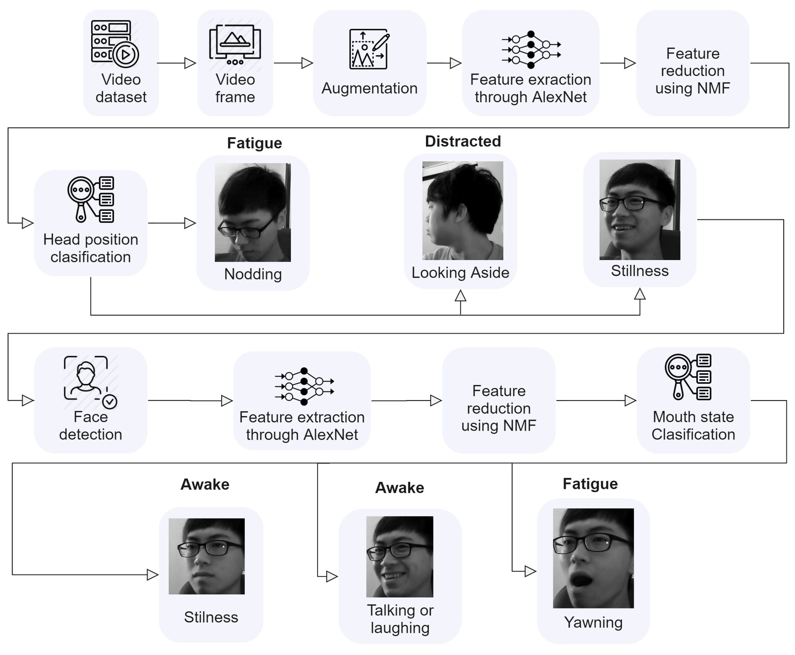
Since our work is concerned with utilizing deep neural pre-trained networks, the following research studies adopted this approach. In [38], the authors extracted features from each eye separately and fed them into a pre-trained CNN model similar to VGG-16 architecture to detect fatigue. The authors were able to achieve an average accuracy of 93.3%.
Other researchers devoted their work to identifying driver distraction through upper body behavior. Y. Xing et al. [39] compared the classification of seven driving behaviors with different models where the pre-trained CNN was fine-tuned and where the pre-trained CNN was used as a feature extractor. For the first approach, the authors used two types of input images, which were Gaussian mixture model (GMM) segmented images and raw images. These images were then trained on pre-trained AlexNet, GoogLeNet and ResNet models. The experiment’s results showed that GMM-based AlexNet achieved the best activity recognition classification results—81.6%. However, when relying on a binary classification to indicate if the driver was distracted or not, the best classification result was found for GMM-based AlexNet, with 94.2% average accuracy.
Similarly, Sarfaraz Masood et al. [40] used pre-trained VGG-16 CNNs to identify ten driving distraction behaviors. They were able to identify distraction behaviors with accuracy of up to 99.5%. Similarly, Yuxin Zhang et al. [41] utilized various information from different sources to identify driver distraction, including facial behaviors, where a camera was used to detect head orientation and eye gaze. The proposed convolutional-LSTM-based model partially used transfer learning and MobileNet was utilized for the data-type images, achieving an accuracy of up to 97.47%. Finally, a summary of the previously mentioned literature is provided in Table 1.
Based on the provided literature, we propose a non-invasive driver fatigue detection model, aiming to reduce computational complexity while improving detection accuracy, as presented in the following section.

3. Methodology

The current section provides an overview of the proposed SVM-based transfer deep learning model, which aims to detect driver fatigue and distraction symptoms. Figure 1 shows the block diagram of the proposed system. Each component is described in detail in the following sections.
As illustrated in Figure 1, video frames were taken from the NTHU drowsy driving video dataset. These frames were preprocessed and fed into a pre-trained AlexNet CNN. Consequently, a feature representation of the training dataset was produced. Then, the NMF was used for the dimension reduction of the feature set, increasing the speed of model training and reducing storage and computational time. The reduced feature set was used as an input to train an SVM classifier. In the proposed model, the driver’s head position is classified to detect the focus of the driver. The head position was chosen as it is the easiest and fastest indicator to detect. The model shows that the driver is visually distracted if he/she is looking away from the road. In another case, if the model identifies fatigue, then the classification has detected that the driver’s head was nodding. However, if the driver’s head is still, the model goes to the next stage and checks the facial features. After using the face detection algorithm, images were fed into another AlexNet pre-trained model, where the facial features were extracted, then reduced and classified through an SVM classifier. The mouth region was chosen for the second classification. If the driver’s mouth is still, talking or laughing, the model assumes that the driver is awake. However, if the driver is yawning, then the model reports it as fatigue.
The following section provides background knowledge on the primary concepts employed in our proposed model.

4. Background Knowledge

4.1. Convolutional Neural Networks

CNNs function as feed-forward networks designed for analyzing and classifying visual data [42]. There are essential factors that have made neural networks well known and successful, such as the availability of large-scale public images and video datasets [43], as well as the invention of high-performance computing (HPC), including graphical processing units and distributed clusters [44]. Overall, the CNN has shown effective results with feature extraction and pattern identification problems [43,45].

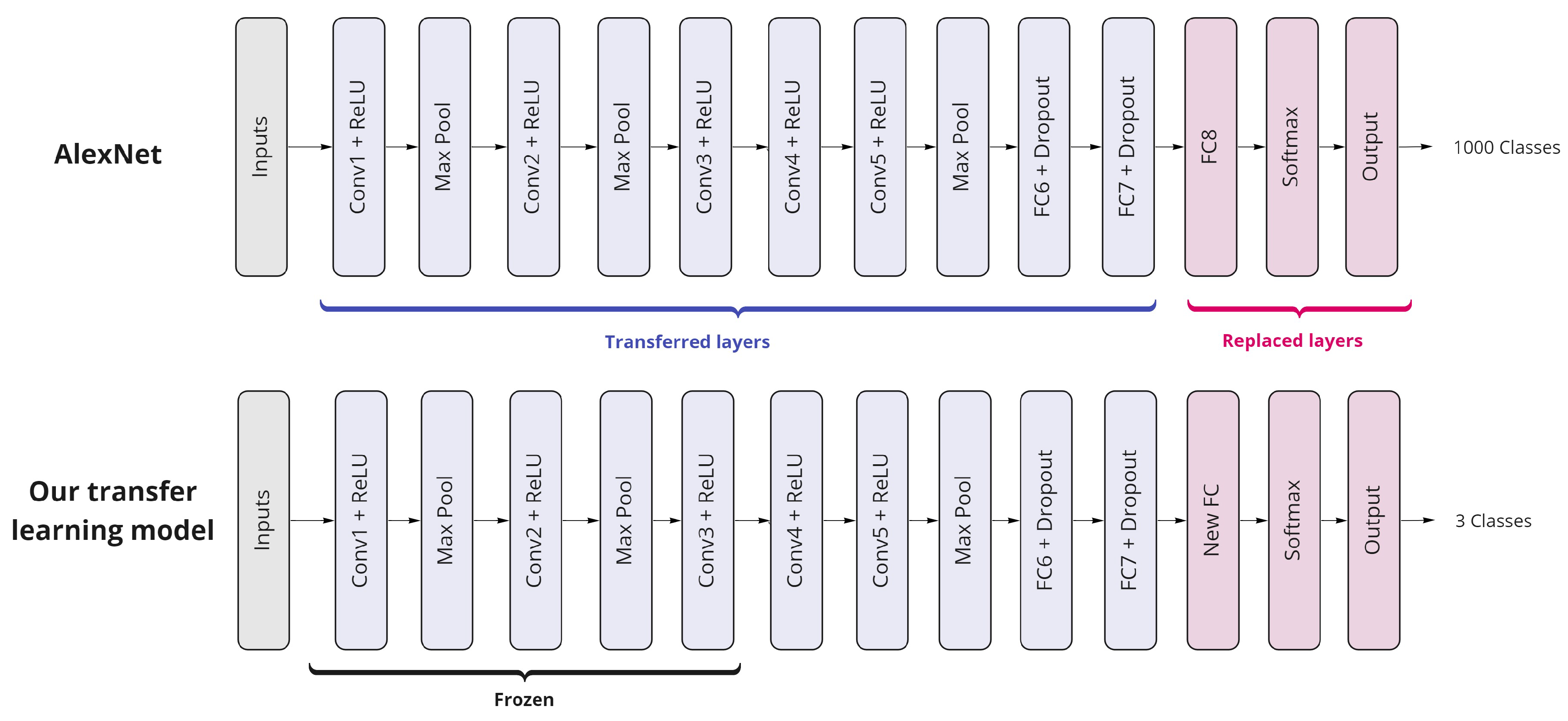
4.2. Pre-Trained Networks and Transfer Learning

Transfer learning is considered a well-known machine learning method, whereby new models can gain knowledge and experience from a previously learned task to improve performance in a new one. The purpose of transfer learning in deep learning is to save time and resources by avoiding the need to train multiple neural network architectures from scratch to fulfill similar tasks. Transfer learning has already been applied to solve problems in various fields, including, but not limited to, speech recognition tasks [46], medical diagnosis tasks [47], human action recognition tasks [48], emotion recognition tasks [49] and climate change and cloud classification [50], as well as road safety systems [45,51]. Building and training a new convolutional neural network from scratch consumes much time and effort. Therefore, pre-trained models are widely used as they provide a better starting point and have a higher learning rate, taking advantage of previously acquired knowledge. Deep pre-trained neural networks can be applied in two ways, i.e., transfer learning by retaining the original pre-trained network while altering the weights to adapt to the new dataset and using the pre-trained network for feature extraction and utilize these features to train a machine learning classifier, such as SVM. Both approaches are widely used. However, the second approach has considerable success in image recognition and classification tasks [48]. Our proposed model falls within the second approach. A few well-known pre-trained networks were trained on a large-scale dataset with millions of images and could classify thousands of objects. The pre-trained network characteristics affect the choice of selecting a network to use. Although VGG16 has high accuracy, the memory requirement is more than twice the consumption needed for AlexNet, since it has about 138 million parameters, as opposed to AlextNet, with 62 million parameters. Additionally, AlexNet has the least computational power among other transfer networks in terms of the number of floating point operations (FLOPs) required to run a forward pass. For this reason, AlextNet was chosen since it provided good attributes in terms of speed, accuracy and size.

4.3. AlexNet

AlexNet is a convolutional neural network that was created by Alex Krizhevsky and his team of researchers. Thanks to its pre-trained neural structure, it is capable of quickly identifying more than a thousand objects. AlexNet was trained on the ImageNet database, which contains ten million images and is categorized into nearly 22 thousand categories. Its goal is to allow researchers to access a valuable image dataset to help them with their studies. Since 2010, ImageNet has held a competition for object recognition called the ImageNet Large Scale Visual Recognition Challenge (ILSVRC). In 2012, Krizhevsky et al. achieved the lowest error rate of 15.3% in ILSVRC, winning first place [52]. Some essential features made AlextNet stand out from other competitors, such as the rectified linear units (ReLUs), which allowed a large model to train six times faster than the standard Tanh units [43]. Additionally, the use of multiple GPUs also significantly improved the model training time. Moreover, the possibility of overfitting in AlextNet is slim due to the introduction of overlapping pooling, which reduced the error by 0.5%. In addition, Alex Krizhevsky et al. minimized overfitting using data augmentation and dropout [43].
AlexNet has a total of eight layers with 62.3 million learnable parameters. It has five convolutional layers combined with max-pooling layers, three fully connected layers and two dropout layers. In addition, the ReLU is the activation function of all layers, except the final output layer, where the Softmax activation function is used. As shown by the architecture in Table 2, as we go deeper, the number of filters is increased to allow the extraction of more features. On the other hand, the size of the filters is reduced to decrease the shape of the filter map. Moreover, since AlexNet is a deep network model, Krizhevsky et al. added padding to maintain the feature maps’ size at a significantly reduced level.

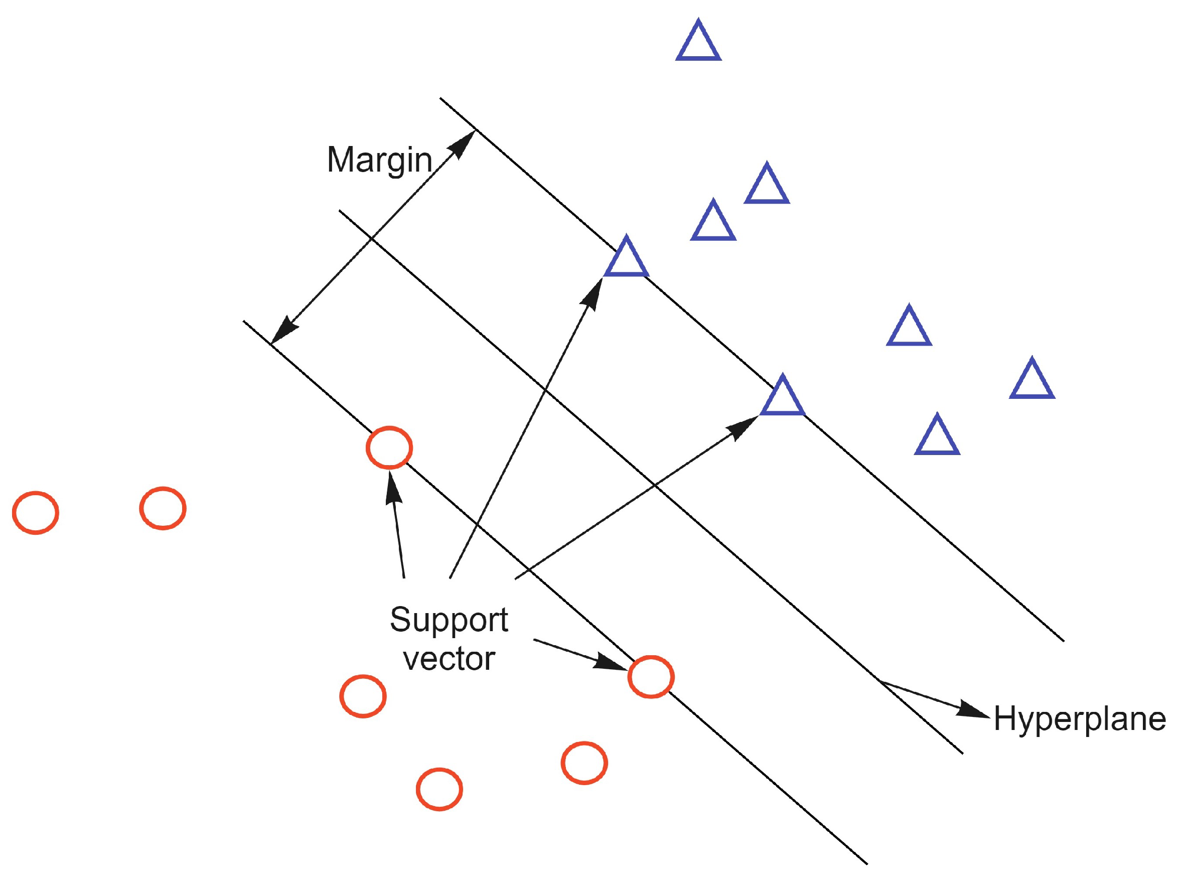
4.4. Support Vector Machine

The support victor machine is considered one of the most common supervised learning models in machine learning. Cortes and Vapnik created SVM and initially meant it to solve binary classification problems [53]. Nonetheless, it became a powerful method to classify linear and non-linear tasks, perform regression and detect outliers. The basic concept of SVM is assigning data points in a non-linear fashion to a highly dimensional feature space by applying the suitable kernel function with the hope of separating data into classes by creating lines or hyperplanes, as illustrated in Figure 2.

5. Implementation

In this work, two pre-trained CNN-based methods were used to classify images from the NTHU driver drowsiness dataset. The first method uses transfer learning based on AlexNet, whereas the second method uses AlexNet as a feature extractor based on SVM. Both models’ structure, implementation and evaluation are explained in detail in the following sections.

5.1. Dataset Description

The dataset used in this study is the Driver Drowsiness Detection dataset collected by National Tsuing Hua University (NTHU) in the computer vision lab [54]. Thirty-six subjects participated in recording a total of 9.5 h in a driver simulation environment to create training, evaluation and testing datasets. Participants were requested to record driving scenarios in changing conditions, such as wearing and removing glasses/sunglasses in the day and at night. Furthermore, drivers performed different behaviors to show their drowsiness status, as elaborated in Table 3. Videos in the dataset were acquired using active infrared illumination, which is convenient for night vision recording. The resolution of the videos was 640 × 480 in AVI and had a frame rate of 15 frames per second (fps) for night videos and 30 fps for daytime videos. Figure 3 and Figure 4 represent sample images for the same behavior but changing conditions and for different behaviors but similar conditions, respectively.

5.2. Dataset Preprocessing and Augmentation

First, frame extraction was applied with a frame rate of 30 fps to the video dataset to acquire the images. At the same time, the label was added to the image from the corresponding annotation file of each video. Afterward, we used the Viola–Jones algorithm [55], which converts images to the grey scale to reduce processing. The algorithm works by relying on Haar features to enable face detection. Viola and Jones identified three types of Haar-like features in their research, edge, line and four rectangle features. The horizontal and vertical features are essential for face detection as they simulate the eyebrows and nose shape, as shown in Figure 5. Consequently, calculated integral images underwent Adaboost training to properly locate and identify facial features. Furthermore, the cascading classifier was used to distinguish whether a window contained a face or not. The upside of using the Viola–Jones algorithm is the real-time processing ability, as well as the robustness, since it has a highly accurate detection rate.
We separated the images to form two different datasets, head and mouth. The classes of each dataset are represented in Table 4. Another equally important image processing technique is image augmentation. By applying image augmentation to the training data, the count of input images can be effectively increased. Augmentation also ensures consistency in the trained network and allows it to overlook distortions in image data. Since our proposed model uses the AlexNet deep transfer model, we applied image augmentation by resizing the dataset to match the standard input image size of AlexNet, which is 227 × 227 × 3, where 3 is the RGB color channels.

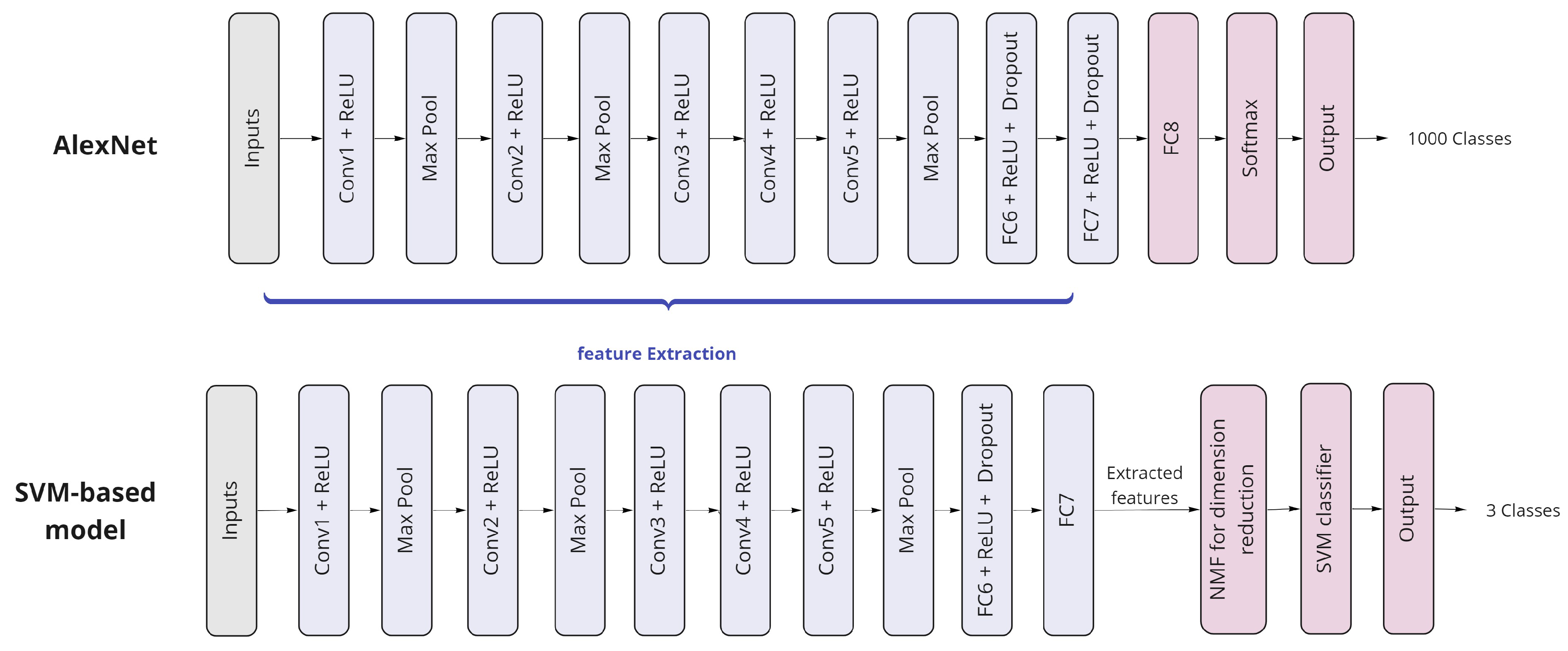
5.3. AlexNet as a Deep Transfer Learning Model

We used the pre-trained AlextNet architecture as the base for our transfer learning model based on two datasets: (1) the head position dataset, which contains three classes, i.e., looking to the side, nodding and stillness; (2) the mouth movement dataset, which contains three classes, i.e., yawning, talking and laughing, and stillness. We began by loading the pre-trained network. Afterward, 80% of the augmented dataset images were used for training, 10% for validation and 10% for testing. Then, we replaced the last three layers in the original AlexNet architecture with new layers to match our three-class output instead of the existing thousand class output. The removed layers were FC8, Softmax and the output layer. The newly added layers were a new FC layer, the Softmax layer and a new output layer, as illustrated in Figure 6. The function of Softmax in the output layer is the classification of facial images. It works by converting real values to probabilities by computing the exponential of a particular class over the sum of the exponential of each class. Consequently, the highest probability was considered as the actual output. Moreover, the cross-entropy loss function was combined with Softmax to determine how well the neural networks fit the data, as defined in Equation (1), where M is the number of classes.
C = 1 M Obsearved C × log ( Predicted C )

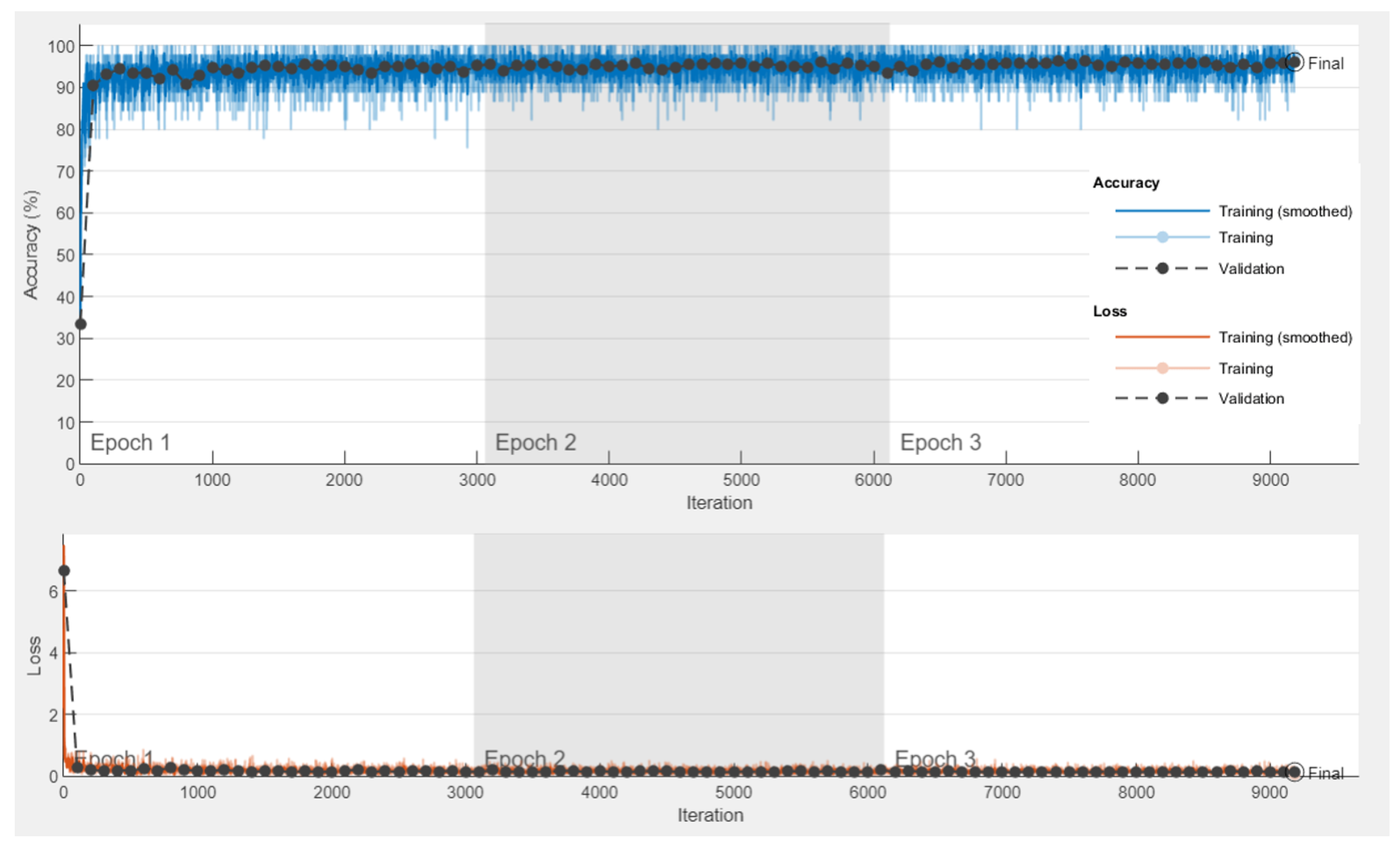
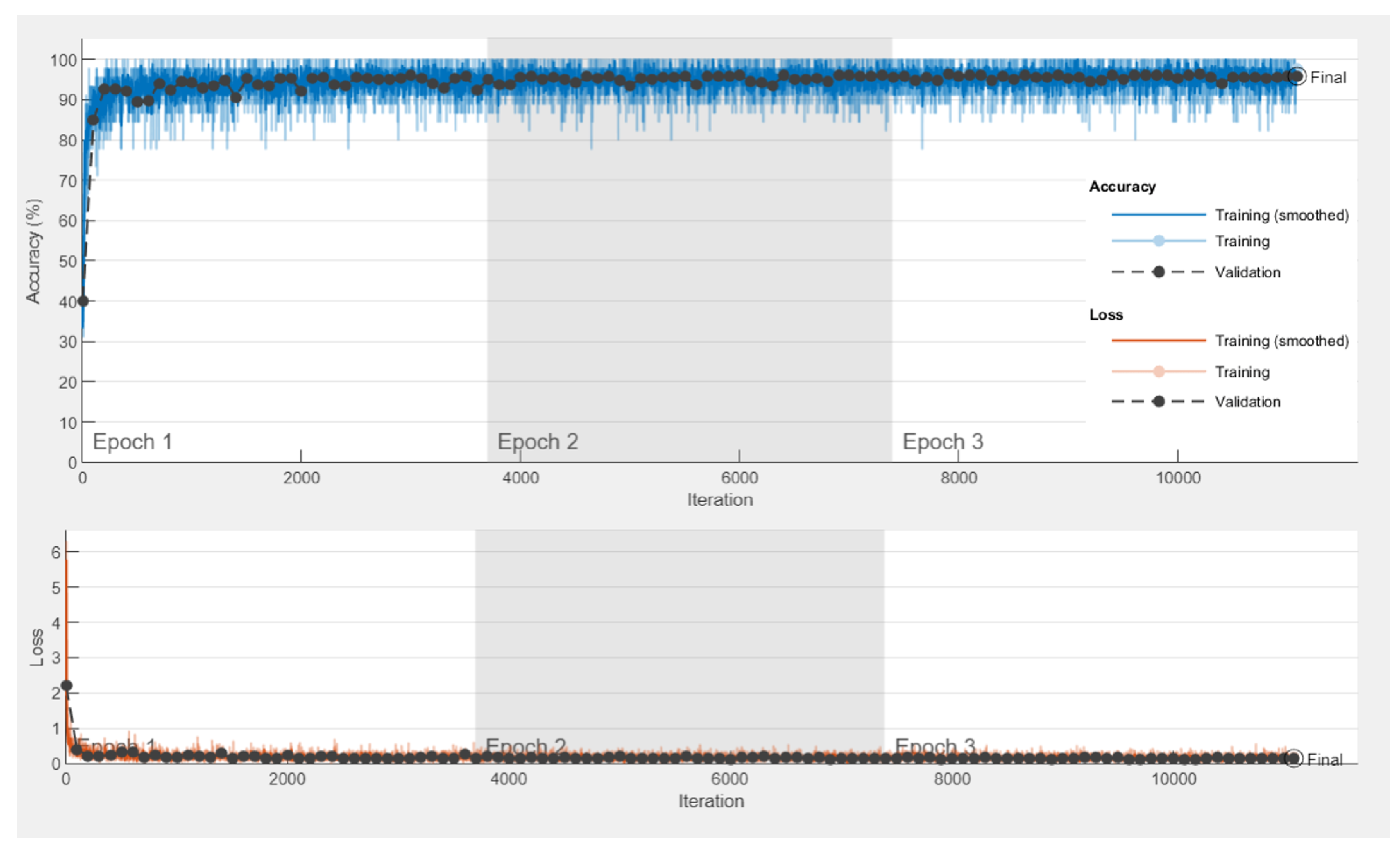
5.3.1. The Experiment of the Transfer Learning-Based Model

All the experiments in this study were conducted using an Intel Core i7-9750H laptop with NVIDIA GeForce GTX 1660 Ti GPU and 16 GB of memory.
After constructing the new model, we set the learning rate to zero in the initial layers, specifically until the third convolutional layer. This process is called weight freezing. As a result, the training time was reduced as the gradients for the frozen layers were not computed, allowing the features obtained from ImageNet to be transferred to our model. The head and mouth datasets were trained separately using the Adam optimizer (adaptive moment estimation), which is one of the most powerful and widely used optimization algorithms in deep learning, as it combines the advantages of RMSProp and momentum optimizers. It reserves the exponentially weighted average of the preceding derivatives, such as momentum, and the preceding squared derivatives, such as RMSProp [56]. Since we applied transfer learning, we did not need a large number of epochs. Therefore, we set the maximum epochs to three. The training dataset was split into mini-batches of 45 and the initial learning rate was set to 0.0003 during training. The hyperparameter of the model is presented in Table 5. Moreover, the model validated the network every 100 iterations. To balance the count of images, training was carried out on the head and mouth datasets, containing nearly 57 thousand and 69 thousand images in each class, respectively, as shown in Table 6.

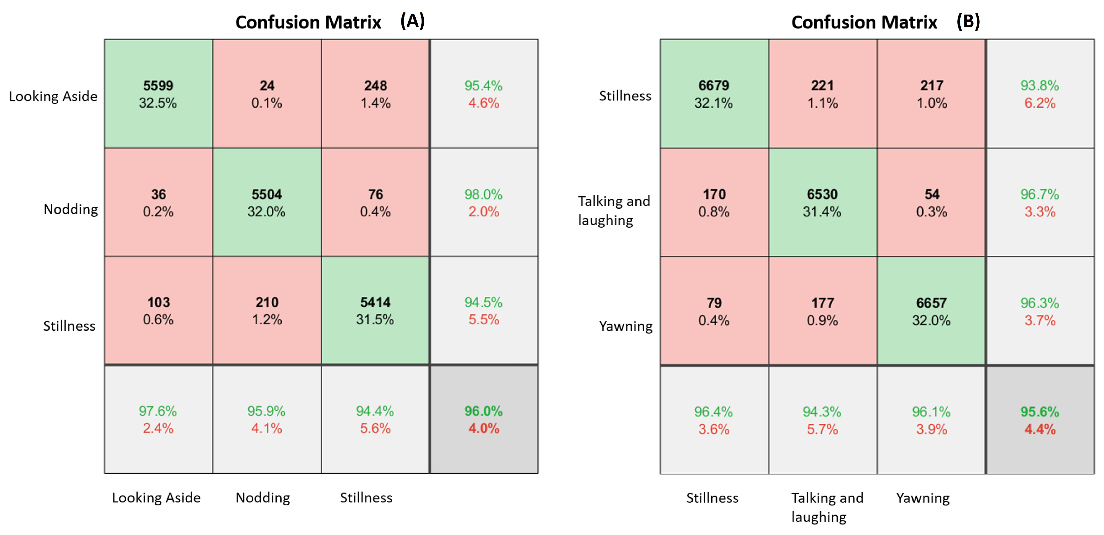
5.3.2. Experimental Results

This section presents the accuracy and performance of the transfer learning model. As illustrated in Figure 7 and Figure 8, the model that classified head positions attained a test accuracy of 95.9% and the model that classified mouth movements achieved a test accuracy of 95.5%.

5.3.3. Performance Metrics

Based on the confusion matrix shown in Figure 9, few performance metrics were derived, namely, (1) PPV (positive predictive value), also called precision, which displays the number of relevant selected cases (2); (2) recall, which indicates how many relevant cases the model properly detected (3); (3) specificity, which shows how many of the model’s actual negative cases were correctly identified (4); (4) FDR (false discovery rate), which is the complement of PPV and shows how many false positive cases were identified (5); (5) the F1-score, which is the mean PPV and recall (6). Moreover, the average results are shown in Table 7.
Recall = True Positive True Positive + False Negative
Specificity = True Negative True Negative + False Psitive
FDR = False Positive False Positive + True Positive
F 1 Score = 2 × Precision × Recall Precision + Recall

5.4. AlexNet as a Feature Extractor with SVM Classifier Model

In this model, the AlexNet pre-trained CNN is used as an image feature extractor. These features are then used as an input to train a machine learning classifier, such as SVM. An illustration of the model representation is shown in Figure 10. This approach is one of the easiest and most efficient methods of employing CNNs, as it saves a lot of the training time since the model goes through the data only once. In this model, the pre-trained CNN was fed a sample of the images from each class, approximately 3000 images for both the head position and the mouth movement datasets, as presented in Table 8. The learned features were extracted from the deeper layers, specifically, the second fully connected layer, which is referred to as fc7 in Figure 10. We chose to extract the features from this layer since it had high-level features learned from earlier layers. The output feature map has a dimension of n × 4096, where n is the number of elements and 4096 represents the number of extracted features. At this stage, we required a dimension reduction technique. Therefore, the NMF function was used.

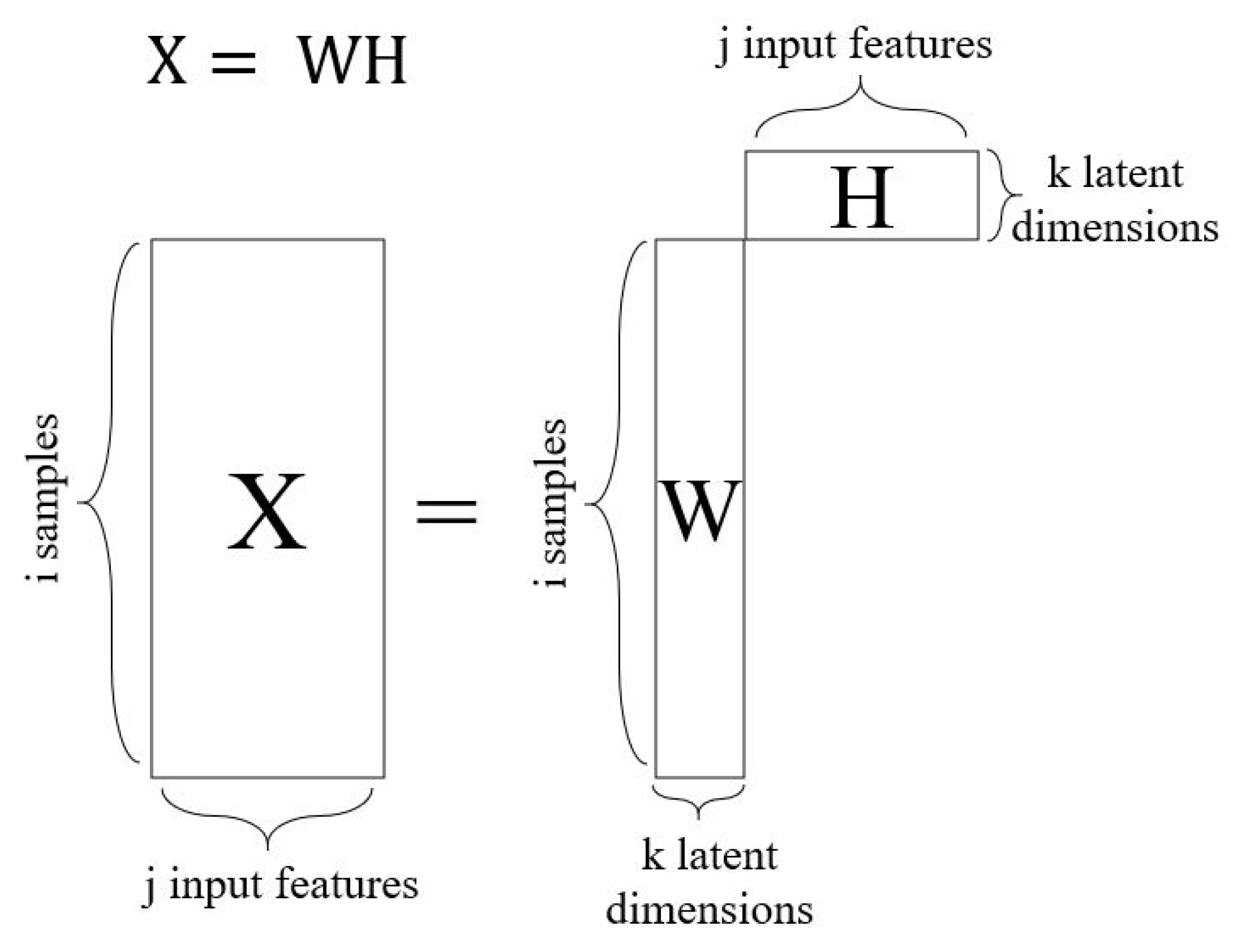
5.4.1. Non-Negative Matrix Factorization

The non-negative matrix factorization is a well-known tool created by Lee and Seung [57]. NMF aims to analyze high-dimensional data and extract distinctive features from a set of non-negative vectors. Basically, NMF factorizes a matrix X with dimensions i × j into two non-negative matrices, matrix W of size i × k and matrix H of size k × j, as shown in Equation (7).
X ( i , j ) W ( i , k ) H ( k , j )
where non-negative matrix X represents the extracted features from all the pixels of the input image; furthermore, the positive integer k has a value of k < min(i, j), where k values represent the resulting columns and rows of W and H, respectively, as shown in Figure 11.
NMF has the ability to minimize the cost function, which is the square of the Euclidean distance between X and WH. To this end, NMF applies a multiplicative update algorithm, which is based on the gradient descent optimization algorithm with different multiplicative update rules. Lee and Seung proved that the gradient descent could converge the minimization problem in a limited number of iterations [58].
The previous section highlights that NMF is used for dimension reduction. However, to obtain the optimal feature value (k) that optimized our model performance, we experimented with our model using a different combination of k values (from 20 to 60). Moreover, we compared the performance against different classifiers, optimizable SVM, optimizable tree and optimizable KNN. The training was carried out for 100 iterations using Bayesian optimization. Regarding the validation, we applied a five-fold cross-validation technique. The configurations are presented in Table 9.

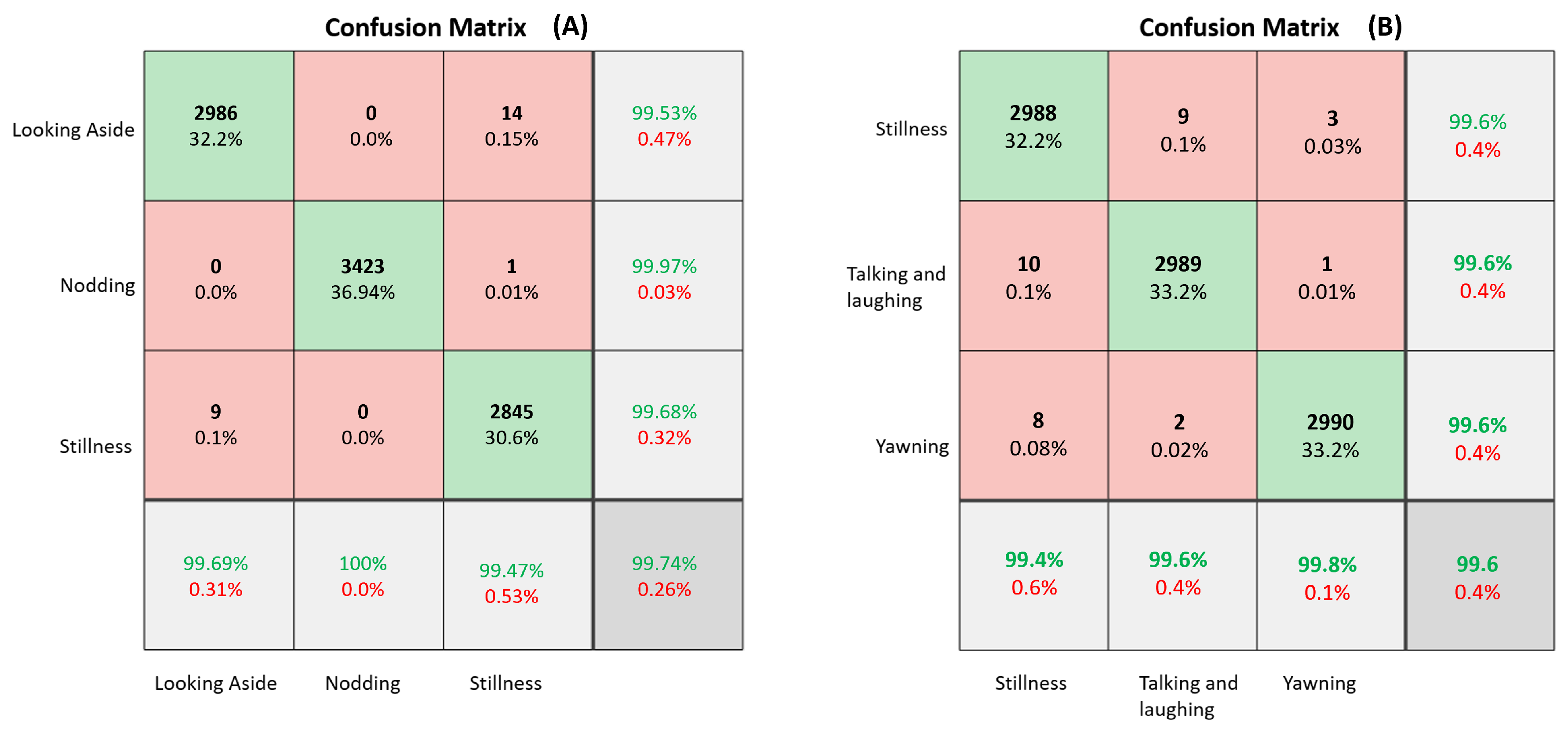
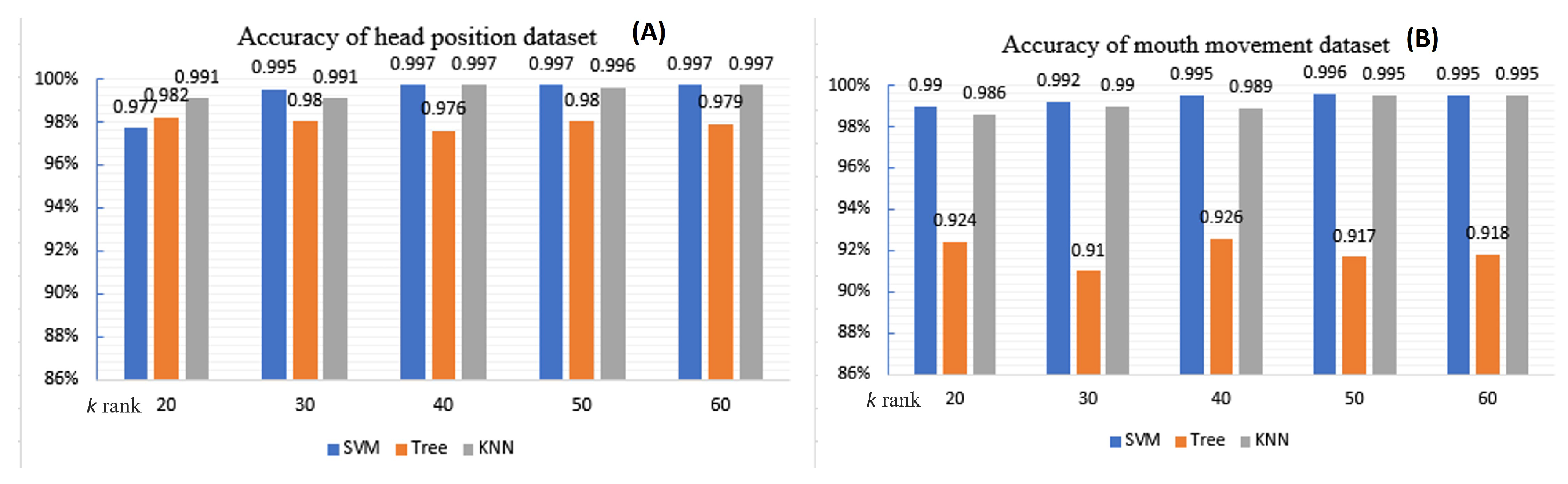
5.4.2. Experimental Results

This section presents the training results of the feature extraction and reduction model. Different reduced feature values for NMF were selected, ranging from 20 to 60, in combination with one of the classifiers. As shown in Figure 12, the SVM and the KNN classifiers had a higher classification accuracy than the tree classifier. However, we chose to work with SVM as it was slightly better and converged faster. Based on all the experiments, we conclude that the best number of selected features is between 40 and 50. Therefore, the performance metrics for the two best models that achieved the highest results are presented below in Table 10. In addition, the corresponding confusion matrix for each of the head position and mouth movement datasets are shown in Figure 13.

6. Discussion

Although the choice of the dataset depended mainly on public availability, we found that the NTHU dataset is diverse in terms of ethnicity. It was found to simulate day and night conditions with and without glasses. This allowed our experiments to be applicable to real-life conditions. However, it is yet to be tested on a real-life driving dataset. Moreover, the purpose of the technique of detecting the mouth movements from the entire face was to learn the facial features, such as the eyes, while the driver is yawning, or talking and laughing, making our model less dependent on a single feature. From the analysis of different transfer learning approaches, we found that, by using AlexNet as a feature extractor in combination with NMF dimension reduction and the SVM classifier, we were able to improve driver fatigue detection performance, producing an average accuracy of 99.65%. In other words, we can say that our proposed model based on AlextNet feature extraction outperformed the AlexNet transfer learning approach in contrast to other works, such as [39], where a comparison was made between transfer learning and the feature extraction approach and the authors found that the feature extraction method did not perform as well as the transfer learning methods in identifying the driver’s behaviors. Moreover, we compared our proposed model with other research studies that used the NTHU dataset, as shown in Table 11.

7. Conclusions

Among the existing work for driver fatigue detection, we introduce a non-invasive approach based on the fusion of features from the driver’s head position and mouth movements. Our work utilized pre-trained neural networks, specifically, the AlexNet CNN. Based on the conducted experiments on the NTHU dataset, we found that, by using AlexNet as a feature extractor and NMF for dimension reduction followed by an SVM classifier, we were able to achieve a high detection accuracy of up to 99.65%. Our approach was compared with transfer learning with fine-tuning of AlexNet. However, it did not yield a higher accuracy than our proposed model. In future work, we suggest testing the model on a real driving conditions’ dataset.

Author Contributions

Conceptualization, S.A. and W.S.; Data curation, S.A.; Formal analysis, S.A., W.A. and W.S.; Investigation, S.A. and W.S.; Methodology, S.A. and W.S.; Project administration, W.A. and W.S.; Software, S.A.; Supervision, W.A. and W.S.; Validation, S.A. and W.S.; Visualization, S.A., W.A. and W.S.; Writing—original draft, S.A.; Writing—review & editing, S.A., W.A. and W.S.; Funding acquisition, W.A. All authors have read and agreed to the published version of the manuscript.

Funding

This research study was funded by The Deanship of Scientific Research (DSR) at King Abdulaziz University, Jeddah, Saudi Arabia, under grant no. FP-211-43.

Institutional Review Board Statement

Not applicable.

Informed Consent Statement

Not applicable.

Data Availability Statement

The dataset used in this study was obtained from Computer Vision Lab, National Tsuing Hua University and are available from the authors at http://cv.cs.nthu.edu.tw/php/callforpaper/datasets/DDD/ (accessed on 3 December 2021) with the permission of National Tsuing Hua University.

Conflicts of Interest

The authors declare no conflict of interest.

References

  1. W.H.O. Global Status Report on Road Safety 2018; World Health Organization: Geneva, Switzerland, 2019; OCLC: 1084537103. [Google Scholar]
  2. Tefft, B.C. Prevalence of motor vehicle crashes involving drowsy drivers, United States, 1999–2008. Accid. Anal. Prev. 2012, 45, 180–186. [Google Scholar] [CrossRef]
  3. Gao, Z.; Wang, X.; Yang, Y.; Mu, C.; Cai, Q.; Dang, W.; Zuo, S. EEG-Based Spatio-Temporal Convolutional Neural Network for Driver Fatigue Evaluation. IEEE Trans. Neural Netw. Learn. Syst. 2019, 30, 1–9. [Google Scholar] [CrossRef]
  4. Zhang, C.; Sun, L.; Cong, F.; Kujala, T.; Ristaniemi, T.; Parviainen, T. Optimal imaging of multi-channel EEG features based on a novel clustering technique for driver fatigue detection. Biomed. Signal Process. Control 2020, 62, 102103. [Google Scholar] [CrossRef]
  5. Tuncer, T.; Dogan, S.; Ertam, F.; Subasi, A. A dynamic center and multi threshold point based stable feature extraction network for driver fatigue detection utilizing EEG signals. Cogn. Neurodyn. 2021, 15, 223–237. [Google Scholar] [CrossRef]
  6. Yang, Y.X.; Gao, Z.K. A Multivariate Weighted Ordinal Pattern Transition Network for Characterizing Driver Fatigue Behavior from EEG Signals. Int. J. Bifurc. Chaos 2020, 30, 2050118. [Google Scholar] [CrossRef]
  7. Wang, F.; Wu, S.; Zhang, W.; Xu, Z.; Zhang, Y.; Chu, H. Multiple nonlinear features fusion based driving fatigue detection. Biomed. Signal Process. Control 2020, 62, 102075. [Google Scholar] [CrossRef]
  8. Shalash, W.M. A Deep Learning CNN Model for Driver Fatigue Detection Using Single Eeg Channel. In Proceedings of the IEEE International Conference on Imaging Systems and Techniques, New York, NY, USA, 24–26 August 2021. [Google Scholar]
  9. Gu, X.; Zhang, L.; Xiao, Y.; Zhang, H.; Hong, H.; Zhu, X. Non-contact Fatigue Driving Detection Using CW Doppler Radar. In Proceedings of the 2018 IEEE MTT-S International Wireless Symposium (IWS), Chengdu, China, 6–10 May 2018; pp. 1–3. [Google Scholar] [CrossRef]
  10. Murugan, S.; Selvaraj, J.; Sahayadhas, A. Detection and analysis: Driver state with electrocardiogram (ECG). Phys. Eng. Sci. Med. 2020, 43, 525–537. [Google Scholar] [CrossRef]
  11. Cherian, V.A.; Bhardwaj, R.; Balasubramanian, V. Real-Time Driver Fatigue Detection from ECG Using Deep Learning Algorithm. In Ergonomics for Improved Productivity; Muzammil, M., Khan, A.A., Hasan, F., Eds.; Springer: Singapore, 2021; pp. 615–621. [Google Scholar]
  12. Chieh, T.C.; Mustafa, M.M.; Hussain, A.; Hendi, S.F.; Majlis, B.Y. Development of vehicle driver drowsiness detection system using electrooculogram (EOG). In Proceedings of the 2005 1st International Conference on Computers, Communications, & Signal Processing with Special Track on Biomedical Engineering, Kuala Lumpur, Malaysia, 14–16 November 2005; pp. 165–168. [Google Scholar] [CrossRef]
  13. Jiao, Y.; Deng, Y.; Luo, Y.; Lu, B.L. Driver sleepiness detection from EEG and EOG signals using GAN and LSTM networks. Neurocomputing 2020, 408, 100–111. [Google Scholar] [CrossRef]
  14. Boon-Leng, L.; Dae-Seok, L.; Boon-Giin, L. Mobile-based wearable-type of driver fatigue detection by GSR and EMG. In Proceedings of the TENCON 2015—2015 IEEE Region 10 Conference, Macao, China, 1–4 November 2015; pp. 1–4. [Google Scholar] [CrossRef]
  15. Satti, A.T.; Kim, J.; Yi, E.; Cho, H.Y.; Cho, S. Microneedle Array Electrode-Based Wearable EMG System for Detection of Driver Drowsiness through Steering Wheel Grip. Sensors 2021, 21, 5091. [Google Scholar] [CrossRef] [PubMed]
  16. Wali, M.K. Ffbpnn-based high drowsiness classification using EMG and WPT. Biomed. Eng. Appl. Basis Commun. 2020, 32, 2050023. [Google Scholar] [CrossRef]
  17. Chen, P. Research on driver fatigue detection strategy based on human eye state. In Proceedings of the 2017 Chinese Automation Congress (CAC), Jinan, China, 20–22 October 2017; pp. 619–623. [Google Scholar] [CrossRef]
  18. Wang, Y.; Huang, R.; Guo, L. Eye gaze pattern analysis for fatigue detection based on GP-BCNN with ESM. Pattern Recognit. Lett. 2019, 123, 61–74. [Google Scholar] [CrossRef]
  19. Fatima, B.; Shahid, A.R.; Ziauddin, S.; Safi, A.A.; Ramzan, H. Driver Fatigue Detection Using Viola Jones and Principal Component Analysis. Appl. Artif. Intell. 2020, 34, 456–483. [Google Scholar] [CrossRef]
  20. Savas, B.K.; Becerikli, Y. Real Time Driver Fatigue Detection System Based on Multi-Task ConNN. IEEE Access 2020, 8, 12491–12498. [Google Scholar] [CrossRef]
  21. Zhang, W.; Su, J. Driver yawning detection based on long short term memory networks. In Proceedings of the 2017 IEEE Symposium Series on Computational Intelligence (SSCI), Honolulu, HI, USA, 27 November–1 December 2017; pp. 1–5. [Google Scholar] [CrossRef]
  22. Yang, H.; Liu, L.; Min, W.; Yang, X.; Xiong, X. Driver Yawning Detection Based on Subtle Facial Action Recognition. IEEE Trans. Multimed. 2021, 23, 572–583. [Google Scholar] [CrossRef]
  23. Hari, C.; Sankaran, P. Driver distraction analysis using face pose cues. Expert Syst. Appl. 2021, 179, 115036. [Google Scholar] [CrossRef]
  24. Ansari, S.; Naghdy, F.; Du, H.; Pahnwar, Y.N. Driver Mental Fatigue Detection Based on Head Posture Using New Modified reLU-BiLSTM Deep Neural Network. IEEE Trans. Intell. Transp. Syst. 2021, 1–13. [Google Scholar] [CrossRef]
  25. Xu, X.; Rong, H.; Li, S. Internet-of-Vehicle-Oriented Fatigue Driving State. In Proceedings of the 2016 IEEE International Conference on Ubiquitous Wireless Broadband (ICUWB), Nanjing, China, 16–19 October 2016; p. 4. [Google Scholar]
  26. Xi, J.; Wang, S.; Ding, T.; Tian, J.; Shao, H.; Miao, X. Detection Model on Fatigue Driving Behaviors Based on the Operating Parameters of Freight Vehicles. Appl. Sci. 2021, 11, 7132. [Google Scholar] [CrossRef]
  27. Li, R.; Chen, Y.V.; Zhang, L. A method for fatigue detection based on Driver’s steering wheel grip. Int. J. Ind. Ergon. 2021, 82, 103083. [Google Scholar] [CrossRef]
  28. Bakker, B.; Zabłocki, B.; Baker, A.; Riethmeister, V.; Marx, B.; Iyer, G.; Anund, A.; Ahlström, C. A Multi-Stage, Multi-Feature Machine Learning Approach to Detect Driver Sleepiness in Naturalistic Road Driving Conditions. IEEE Trans. Intell. Transp. Syst. 2021, 1–10. [Google Scholar] [CrossRef]
  29. Liu, Z.; Peng, Y.; Hu, W. Driver fatigue detection based on deeply-learned facial expression representation. J. Vis. Commun. Image Represent. 2020, 71, 102723. [Google Scholar] [CrossRef]
  30. Teyeb, I.; Jemai, O.; Zaied, M.; Ben Amar, C. A Drowsy Driver Detection System Based on a New Method of Head Posture Estimation. In Intelligent Data Engineering and Automated Learning–IDEAL 2014; Corchado, E., Lozano, J.A., Quintián, H., Yin, H., Eds.; Lecture Notes in Computer Science; Springer International Publishing: Cham, Germany, 2014; Volume 8669, pp. 362–369. [Google Scholar]
  31. Moujahid, A.; Dornaika, F.; Arganda-Carreras, I.; Reta, J. Efficient and compact face descriptor for driver drowsiness detection. Expert Syst. Appl. 2021, 168, 114334. [Google Scholar] [CrossRef]
  32. Bakheet, S.; Al-Hamadi, A. A Framework for Instantaneous Driver Drowsiness Detection Based on Improved HOG Features and Naïve Bayesian Classification. Brain Sci. 2021, 11, 240. [Google Scholar] [CrossRef] [PubMed]
  33. Li, X.; Xia, J.; Cao, L.; Zhang, G.; Feng, X. Driver fatigue detection based on convolutional neural network and face alignment for edge computing device. Proc. Inst. Mech. Eng. Part J. Automob. Eng. 2021, 235, 2699–2711. [Google Scholar] [CrossRef]
  34. Jabbar, R.; Al-Khalifa, K.; Kharbeche, M.; Alhajyaseen, W.; Jafari, M.; Jiang, S. Real-time Driver Drowsiness Detection for Android Application Using Deep Neural Networks Techniques. Procedia Comput. Sci. 2018, 130, 400–407. [Google Scholar] [CrossRef]
  35. Quddus, A.; Shahidi Zandi, A.; Prest, L.; Comeau, F.J. Using long short term memory and convolutional neural networks for driver drowsiness detection. Accid. Anal. Prev. 2021, 156, 106107. [Google Scholar] [CrossRef]
  36. Jacobé de Naurois, C.; Bourdin, C.; Bougard, C.; Vercher, J.L. Adapting artificial neural networks to a specific driver enhances detection and prediction of drowsiness. Accid. Anal. Prev. 2018, 121, 118–128. [Google Scholar] [CrossRef]
  37. He, H.; Zhang, X.; Jiang, F.; Wang, C.; Yang, Y.; Liu, W.; Peng, J. A Real-time Driver Fatigue Detection Method Based on Two-Stage Convolutional Neural Network. IFAC-PapersOnLine 2020, 53, 15374–15379. [Google Scholar] [CrossRef]
  38. Pinto, A.; Bhasi, M.; Bhalekar, D.; Hegde, P.; Koolagudi, S.G. A Deep Learning Approach to Detect Drowsy Drivers in Real Time. In Proceedings of the 2019 IEEE 16th India Council International Conference (INDICON), Rajkot, India, 13–15 December 2019; pp. 1–4. [Google Scholar] [CrossRef]
  39. Xing, Y.; Lv, C.; Cao, D. Application of Deep Learning Methods in Driver Behavior Recognition. In Advanced Driver Intention Inference; Elsevier: Amsterdam, The Netherlands, 2020; pp. 135–156. [Google Scholar] [CrossRef]
  40. Masood, S.; Rai, A.; Aggarwal, A.; Doja, M.; Ahmad, M. Detecting distraction of drivers using Convolutional Neural Network. Pattern Recognit. Lett. 2020, 139, 79–85. [Google Scholar] [CrossRef]
  41. Zhang, Y.; Chen, Y.; Gao, C. Deep unsupervised multi-modal fusion network for detecting driver distraction. Neurocomputing 2021, 421, 26–38. [Google Scholar] [CrossRef]
  42. Kůrková, V.; Manolopoulos, Y.; Hammer, B.; Iliadis, L.; Maglogiannis, I. (Eds.) Artificial Neural Networks and Machine Learning. In Proceedings of the ICANN 2018: 27th International Conference on Artificial Neural Networks, Rhodes, Greece, 4–7 October 2018; Lecture Notes in Computer Science. Springer International Publishing: Berlin/Heidelberg, Germany, 2018. Part II. Volume 11140. [Google Scholar] [CrossRef]
  43. Krizhevsky, A.; Sutskever, I.; Hinton, G.E. ImageNet classification with deep convolutional neural networks. Commun. ACM 2017, 60, 84–90. [Google Scholar] [CrossRef]
  44. Simonyan, K.; Zisserman, A. Very Deep Convolutional Networks for Large-Scale Image Recognition. arXiv 2015, arXiv:1409.1556. [Google Scholar]
  45. Abbas, Q. HybridFatigue: A Real-time Driver Drowsiness Detection using Hybrid Features and Transfer Learning. Int. J. Adv. Comput. Sci. Appl. (IJACSA) 2020, 11. [Google Scholar] [CrossRef] [Green Version]
  46. Kunze, J.; Kirsch, L.; Kurenkov, I.; Krug, A.; Johannsmeier, J.; Stober, S. Transfer Learning for Speech Recognition on a Budget. arXiv 2017, arXiv:1706.00290. [Google Scholar]
  47. Alyoubi, W.L.; Abulkhair, M.F.; Shalash, W.M. Diabetic Retinopathy Fundus Image Classification and Lesions Localization System Using Deep Learning. Sensors 2021, 21, 3704. [Google Scholar] [CrossRef] [PubMed]
  48. Sargano, A.B.; Wang, X.; Angelov, P.; Habib, Z. Human action recognition using transfer learning with deep representations. In Proceedings of the 2017 International Joint Conference on Neural Networks (IJCNN), Vancouver, QC, Canada, 24–29 July 2017; pp. 463–469. [Google Scholar] [CrossRef] [Green Version]
  49. Kaya, H.; Gürpınar, F.; Salah, A.A. Video-based emotion recognition in the wild using deep transfer learning and score fusion. Image Vis. Comput. 2017, 65, 66–75. [Google Scholar] [CrossRef]
  50. Manzo, M.; Pellino, S. Voting in Transfer Learning System for Ground-Based Cloud Classification. Mach. Learn. Knowl. Extr. 2021, 3, 542–553. [Google Scholar] [CrossRef]
  51. Shalash, W.M. Driver Fatigue Detection with Single EEG Channel Using Transfer Learning. In Proceedings of the 2019 IEEE International Conference on Imaging Systems and Techniques (IST), Abu Dhabi, United Arab Emirates, 9–10 December 2019; pp. 1–6. [Google Scholar] [CrossRef]
  52. Russakovsky, O.; Deng, J.; Su, H.; Krause, J.; Satheesh, S.; Ma, S.; Huang, Z.; Karpathy, A.; Khosla, A.; Bernstein, M.; et al. ImageNet Large Scale Visual Recognition Challenge. Int. J. Comput. Vis. 2015, 115, 211–252. [Google Scholar] [CrossRef] [Green Version]
  53. Cortes, C.; Vapnik, V. Support-vector networks. Mach. Learn. 1995, 20, 273–297. [Google Scholar] [CrossRef]
  54. Weng, C.H.; Lai, Y.H.; Lai, S.H. Driver Drowsiness Detection via a Hierarchical Temporal Deep Belief Network. In Proceedings of the Asian Conference on Computer Vision—ACCV 2016 Workshops, Taipei, Taiwan, 20–24 November 2016; Chen, C.S., Lu, J., Ma, K.K., Eds.; Lecture Notes in Computer Science. Springer International Publishing: Berlin/Heidelberg, Germany, 2016; Volume 10118, pp. 117–133. [Google Scholar]
  55. Viola, P.; Jones, M. Robust Real-time Object Detection. Int. J. Comput. Vis. 2001, 4, 4. [Google Scholar]
  56. Michelucci, U. Applied Deep Learning: A Case-Based Approach to Understanding Deep Neural Networks; Apress: Berkeley, CA, USA, 2018. [Google Scholar] [CrossRef]
  57. Lee, D.D.; Seung, H.S. Learning the parts of objects by non-negative matrix factorization. Nature 1999, 401, 788–791. [Google Scholar] [CrossRef]
  58. Gillis, N. Nonnegative Matrix Factorization: Complexity, Algorithms and Applications. Ph.D. Thesis, Université Catholique de Louvain, Ottignies-Louvain-la-Neuve, Belgique, 2011. Available online: https://dial.uclouvain.be/downloader/downloader.php?pid=boreal:70744&datastream=PDF_01 (accessed on 5 November 2020).
Figure 1. Overview of the proposed model.
Electronics 11 00285 g001
Figure 2. A binary classification of SVM.
Electronics 11 00285 g002
Figure 3. Sample images for the same behavior but changing conditions.
Electronics 11 00285 g003
Figure 4. Sample images for different behaviors in similar conditions.
Electronics 11 00285 g004
Figure 5. Haar-like features.
Electronics 11 00285 g005
Figure 6. The structure of the transfer learning model.
Electronics 11 00285 g006
Figure 7. Training progress of head position dataset.
Electronics 11 00285 g007
Figure 8. Training progress of mouth movement dataset.
Electronics 11 00285 g008
Figure 9. Confusion matrix of the transfer learning model for (A) head position dataset and (B) mouth movement dataset.
Electronics 11 00285 g009
Figure 10. AlexNet as a feature extractor combined with SVM classifier.
Electronics 11 00285 g010
Figure 11. Non-negative matrix factorization.
Electronics 11 00285 g011
Figure 12. Training results of the feature extraction model for classifying (A) head position dataset and (B) mouth movement dataset.
Electronics 11 00285 g012
Figure 13. Confusion matrices of the feature extraction model for (A) the head position dataset and (B) mouth movement dataset.
Electronics 11 00285 g013
Table 1. Summary of the literature review.
CitationGoalUsed MeasuresMethodDatasetPerformance
[29]Detecting driver fatiguePERCLOS YawningRule-basedCaltech10k Web Faces dataset, FDDB datasetSuccess rate under normal conditions: 96.5%
[30]Detecting driver fatigueHead positionRule-basedSelf-built datasetSuccess rate: 88.33%
[23]Detecting driver distractionHead positionTwo-layer clustered approach with Gabor features and SVM classifierSelf-built datasetAccuracy: 95.8%
[32]Detecting driver fatigueEye stateImproved HOG features and NB classifierNTHU Drowsy Driver Detection datasetAccuracy: 85.62%
[31]Detecting driver fatigueFacial featuresFeature extraction through multiple face descriptors followed by PCA and SVMNTHU Drowsy Driver Detection datasetAccuracy: 79.84%
[34]Detecting driver fatigueFacial featuresMulti-layer perceptronNTHU Drowsy Driver Detection datasetAccuracy: 81%
[33]Detecting driver fatigue and distractionEye aspect ratio, mouth aspect ratio, head posesCNN-based face detection network, speed-optimized SDM face alignment algorithmAFLW, Pointing’04, 300W, 300W-LP, Menpo2D, self-built dataset (DriverEyes), YawDD datasetAccuracy: 89.55%
[35]Detecting driver fatigueEye movementLSTM-CNNSelf-built datasetAccuracy: 97.87%
[36]Detecting driver fatigueEye movement, head position, head rotation, heart rate, respiration rate, car dataAdaptive ANNSelf-built dataset80% performance improvement after adaptation of AdANN
[37]Detecting driver fatigueEye state, mouth stateCNNYawDD dataset, Self-built datasetAccuracy: 94.7%
[18]Detecting driver fatigueEye gazeDual-stream bidirectional CNN with projection vectors and Gabor filtersClosed Eyes in the Wild dataset, Eyeblink dataset, self-built datasetAccuracy: 97.9%
[20]Detecting driver fatiguePERCLOS, YawningCNNYawdDD dataset, NTHU Drowsy Driver Detection datasetAccuracy: 98.81%
[38]Detecting driver fatigueEye statePre-trained VGG-16 CNNClosed Eyes in the Wild dataset, self-built datasetAccuracy: 93.3%
[39]Detecting driver distractionUpper body behaviorsPre-trained AlexNet CNNSelf-built datasetAccuracy: 94.2%
[40]Detecting driver distractionUpper body behaviorsPre-trained VGG-16 CNNState Farm Distracted Drivers DatasetAccuracy: 99.5%
[41]Detecting driver distractionHead orientation, eye behavior, skin sensor to detect emotions, car signals, EMGDeep multi-modal fusion based on Conv-LSTM MobileNet CNN is used for images data typeSelf-built datasetAccuracy: 97.47%
Table 2. AlexNet architecture.
TypeNumber of FiltersFilter SizeStridePaddingSize of the Feature MapActivation Function
Input----227 × 227 × 3-
Convolution l9611 × 114-55 × 55 × 96ReLU
Max Pool 1-3 × 32-27 × 27 × 96-
Convolution 22565 × 51227 × 27 × 256ReLU
Max Pool 2-3 × 32-13 × 13 × 256-
Convolution 33843 × 31113 × 13 × 384ReLU
Convolution 43843 × 31113 × 13 × 384ReLU
Convolution 52563 × 31113 × 13 × 256ReLU
Max Pool 3-3 × 32-6 × 6 × 256-
Fully Connected 1----4096ReLU
Dropout 1Rate = 0.5---4096-
Fully Connected 2----4096ReLU
Dropout 2Rate = 0.5---4096-
Fully Connected 3----1000Softmax
Table 3. Drivers’ behaviors from the NTHU dataset.
Driver’s BehaviorDescription
YawningThe participant yawns as an indication of tiredness
NoddingThe participant’s head falls as an indication of feeling sleepy
Looking asideThe participant looks right or left as an indication of distraction
Talking or laughingThe participant makes conversation as an indication of being vigilant
Sleepy eyesThe participant’s eye blinking rate is increasing as an indication of drowsiness
DrowsyThe participant performs a collection of the above behaviors as an indication of drowsiness
StillnessThe participant is still and drives normally
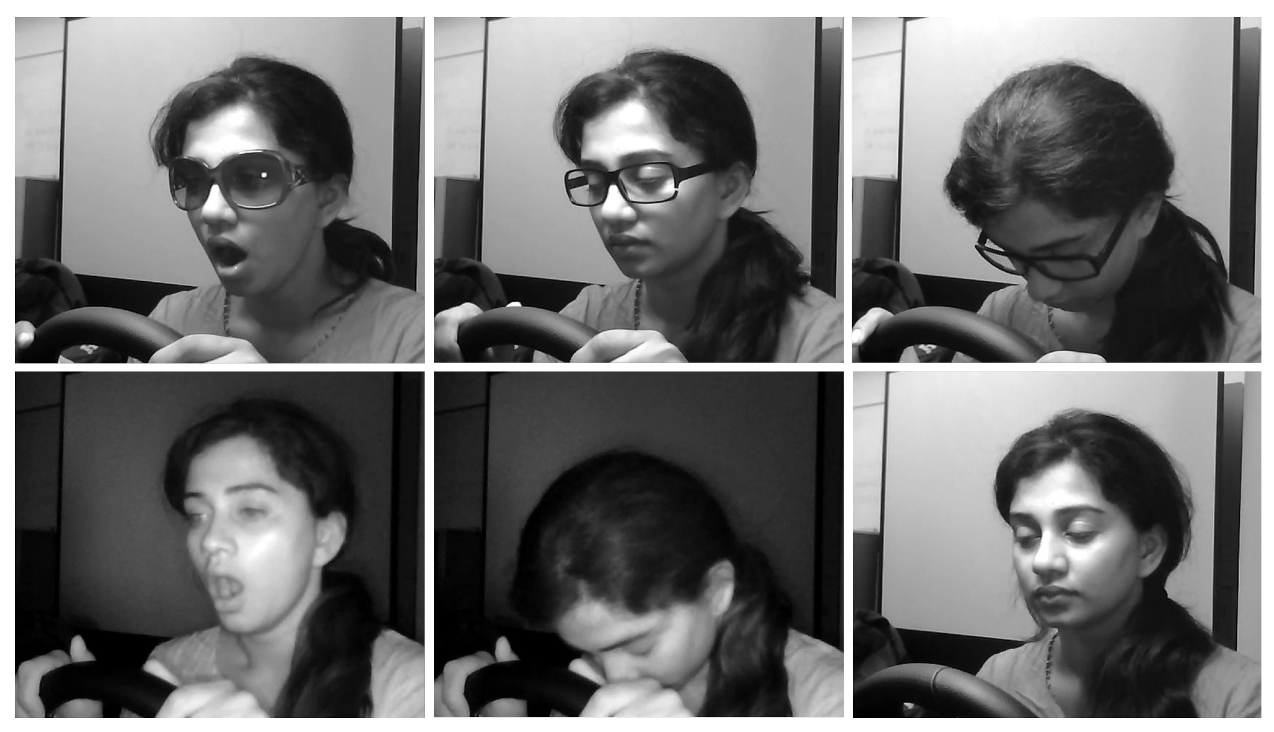
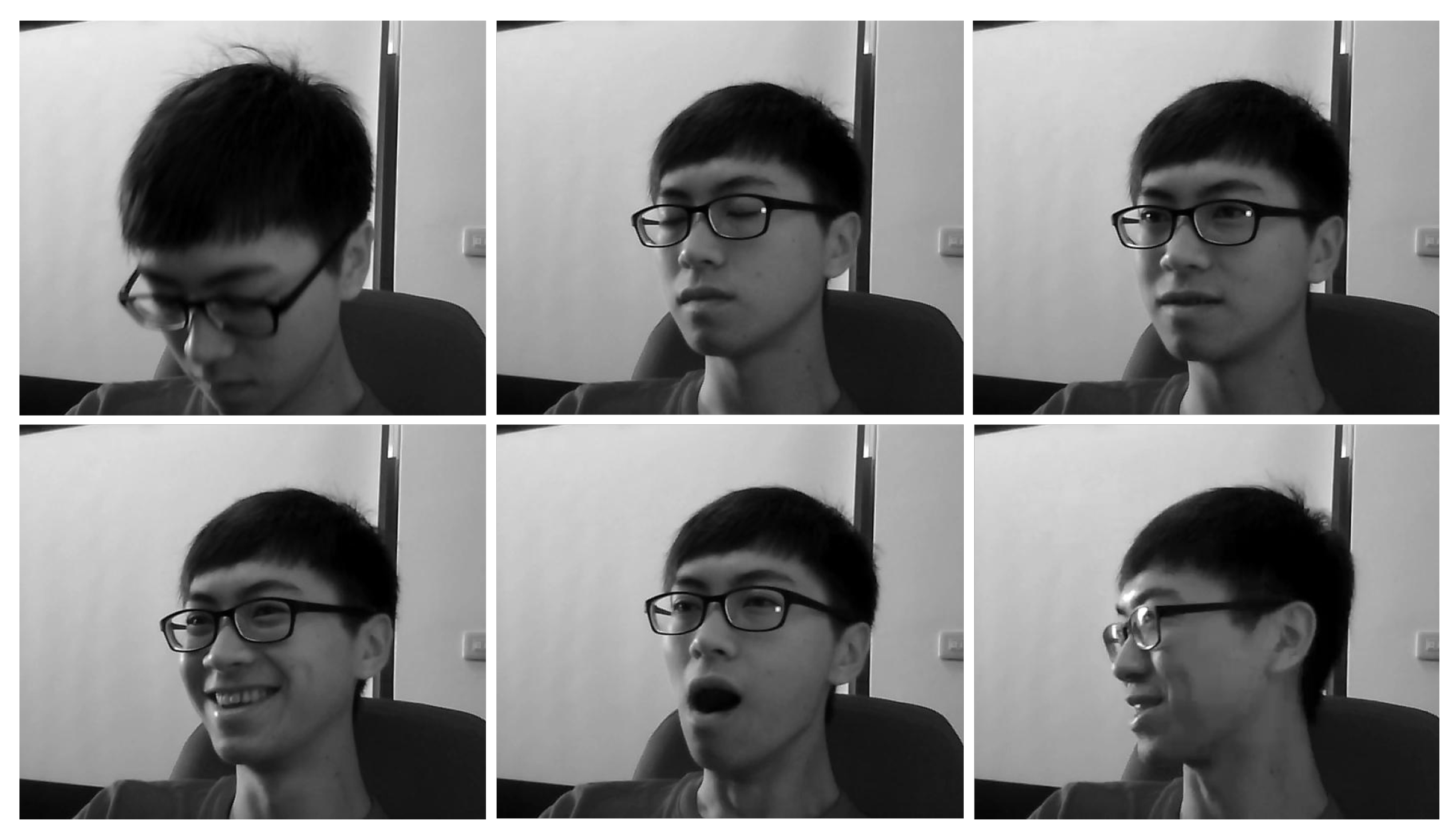
Table 4. Representation of the dataset used.
DatasetClassesDataset AnnotationNumber of SubjectsScenarios
Head PositionStillness036Day—without glasses
Nodding1 Day—glasses
Looking to the side2 Day—sunglasses
Mouth MovementsStillness036Night—without glasses
Yawning1 Night—glasses
Talking and laughing2
Table 5. Hyperparameter configuration for the transfer learning models.
ConfigurationValue
OptimizerAdam optimizer
Mini-batches45
Initial learning rate0.0003
Maximum epochs3
Validation frequencyEvery 100 iterations
L2 regularization0.1
Squared gradient decay factor0.8
Execution environmentmulti-GPU
Table 6. Image count for the transfer learning model.
Head Position DatasetMouth Movement Dataset
Training45,600 images55,200 images
Evaluation5700 images6900 images
Testing5700 images6900 images
Image Size640 × 480640 × 480
Total57,000 images69,000 images
Table 7. Performance metrics of the transfer learning model.
Transfer Learning ModelPPVRecallSpecificityFDRF1-ScoreAccuracy
Transfer learning modelPPVRecallSpecificityFDRF1-scoreAccuracy
Head dataset0.9590.9590.970.040.95995.9%
Mouth dataset0.9550.9580.9770.040.95795.5%
Combined model0.9570.9580.970.040.95895.7%
Table 8. Image count for the feature extraction model.
Head Position DatasetMouth Movement Dataset
3000 looking aside images3000 yawning images
3425 nodding images3000 talking and laughing images
2854 stillness images3000 stillness images
9279 images9000 images
Table 9. Hyperparameter configuration for the feature extraction models.
ConfigurationValue
ClassifierOptimizable SVM, optimizable tree and optimizable KNN
Kernel functionGaussian
OptimizerBayesian optimization
K rank20–60
ValidationFive-fold cross-validation technique
Table 10. Performance metrics of the SVM-based feature extraction model.
Transfer Learning ModelK RankPPVRecallSpecificityFDRF1-ScoreAccuracy
Head dataset400.9970.9970.9980.020.99799.7%
Mouth dataset500.9960.9960.9980.0030.99699.6%
Combined model-0.99650.99650.9980.010.996599.65%
Table 11. Comparing our model with other works.
CitationUsed MeasuresMethodDatasetPerformance
[31]Facial featuresFeature extraction through multiple face descriptors followed by PCA and SVMNTHU Drowsy Driver Detection datasetAccuracy: 79.84%
[32]Eye stateImproved HOG features and NB classifierNTHU Drowsy Driver Detection datasetAccuracy: 85.62%
[34]Facial featuresMulti-layer perceptronNTHU Drowsy Driver Detection datasetAccuracy: 81%
[20]PERCLOS, yawningCNNNTHU Drowsy Driver Detection datasetAccuracy: 98.89%
Our modelHead position, mouth movementsAlexNet feature extraction based on NMF and SVMNTHU Drowsy Driver Detection datasetAccuracy: 99.65%
Publisher’s Note: MDPI stays neutral with regard to jurisdictional claims in published maps and institutional affiliations.

