An Adaptive Modeling Framework for Bearing Failure Prediction

Abstract

Rolling element bearings are a common component in rotating equipment, a class of machines that is essential in a wide range of industries. Detecting and predicting bearing failures is then vital for reducing maintenance and production costs due to unplanned downtime. In previous literature, significant efforts have been devoted to building data-driven health models from historical bearing data. However, a common limitation is that these methods are typically tailored to specific failure instances and have limited ability to model bearing failures between repairs in the same system. In this paper, we propose a multi-state health model to predict bearing failures before they occur. The model employs a regression-based method to detect health state transition points and applies an exponential random coefficient model with a Bayesian updating process to estimate time-to-failure distributions. A model training framework is also introduced to make our proposed model applicable to more bearing instances in the same system setting. The proposed method has been tested on a publicly available bearing prognostics dataset. Case study results show that the proposed method provides accurate failure predictions across several system failures, and that the training approach can significantly reduce the time necessary to generate an effective, generalized model.

1. Introduction

Rotating equipment is widely used in industry applications, with the demand for system reliability continuing to increase. Equipment failures cause unplanned downtime across the system, which can lead to production losses and costly repairs. Rolling element bearings are one of the most common components in modern rotating equipment. During operation, the race and rolling element surfaces within these bearings are subject to a variety of stresses. As a bearing nears the end of its fatigue life, these stresses can cause defects to emerge on bearing surfaces. Continued operation will exacerbate surface defects, a process that can be accelerated by the presence of contaminating particulates or flakes of material from the bearing itself. As a result, degradation in health often develops gradually on the bearings but quickly escalates as the surface defects increase [1]. Approximately 40% to 50% of machine breakdowns are caused by bearing failures [2]. Therefore, it is critical to detect the presence and propagation of faults, and estimate the time to failure (TTF) to prevent unplanned downtime.

Approaches to detect the presence of degradation in bearings and predict imminent failures may be physics-based, if the degradation process and system parameters are well-understood, or data-driven, if failure data for training is available. Previous physics-based approaches have used models that relate vibration characteristics to bearing health based on the size of the bearings surface defects [3] or changes in the stiffness of the bearings that result from surface defects [4]. In these works, experimental tests are necessary to tune the parameters of the dynamic bearing models. A review of similar approaches to modeling bearing failures can be found in [5]. These methods are well-suited for detecting specific bearing failure modes but are often not suitable for general health monitoring. More recently, there have been significant efforts devoted to data-driven approaches for modeling and predicting the failure time of bearings [6,7]. Existing work has modeled bearing degradation as both a series of discrete states [8] and a continuous process [9]. Many different methods for estimating a bearing’s health state and predicting failures during operation have also been proposed, making use of adaptive regression models [10], neural networks [11,12], Kalman filters [13], and hidden Markov models [14]. These data-driven techniques model the dynamical behavior of the monitored bearings in the system, and adjust the model parameters to capture the recent trend of the degradation signals.

Bearing failure modes are predominately characterized by defects on one or more of the bearing’s internal surfaces. In practice, bearing failures can be attributed to wear on the inner race surface, wear on the outer race surface, or wear on the surface of a rolling element. The underlying cause of wear can also be used to describe bearing failure. Two common causes of bearing wear are insufficient lubricant and the presence of foreign particles in the bearing [5]. A limitation of existing approaches is that most of the data-driven models are tailored for specific failure instances of the bearings. Existing models have a limited ability to be applied to varying instances of bearing failure within the same system. Thus, these approaches cannot be used when industrial rotating equipment encounter unanticipated bearing failure modes. Some deep learning methods have shown high accuracy of the TTF prediction for a wide range of bearing instances; however, these methods require a large amount of training data [15,16]. Additionally, these methods cannot retrain or adjust their models when new failure instances are encountered. Such limitations make these methods impractical for implementation in agile manufacturing systems.

In this study, we propose a general multi-state health model for rolling element bearings in rotating equipment that predicts the TTF distribution before failure occurs given historical condition data. The model employs a regression-based method to detect the health state transition points. For the prediction of TTF distribution, we extend the exponential random coefficient model from [17,18] in order to make the model parameters adaptive and fit it into the proposed multi-state health model. Specifically, we develop a linear model during early stages of degradation and then transition it to an exponential model as degradation progresses and we get an understanding from the data of the exponential time constant. Furthermore, to address the limitation of existing works, a model training framework is proposed. It trains the multi-state health model based on historical bearing data, and is able to update the model when new failure instances are encountered.

The first contribution of this work is a general multi-state health model for the purpose of TTF prediction of rolling element bearings. The second contribution is a model training framework to make the proposed model generally applicable to different bearings in the same system and adjustable when the model observes new data.

The rest of this paper is organized as follows: Section 2 explains the general structure of the proposed multi-state health model as well as the method for state transition points detection and TTF prediction. Section 3 describes the proposed model training process. Section 4 introduces the case study on IMS bearing data and obtained results. Finally, Section 5 presents conclusions and proposals for future work.

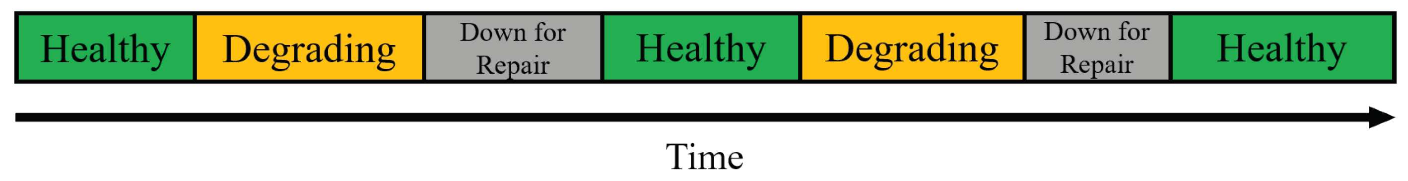
2. Multi-State Health Model

This section presents a general multi-state health model which analyzes historical data of bearings on rotating equipment for the purpose of TTF prediction. In the following parts of this section, we first introduce the general structure of the health model. Next, we describe the methods for state transition point detection. Finally, we present how we predict the TTF distribution using an exponential random coefficient model with Bayesian updating method.

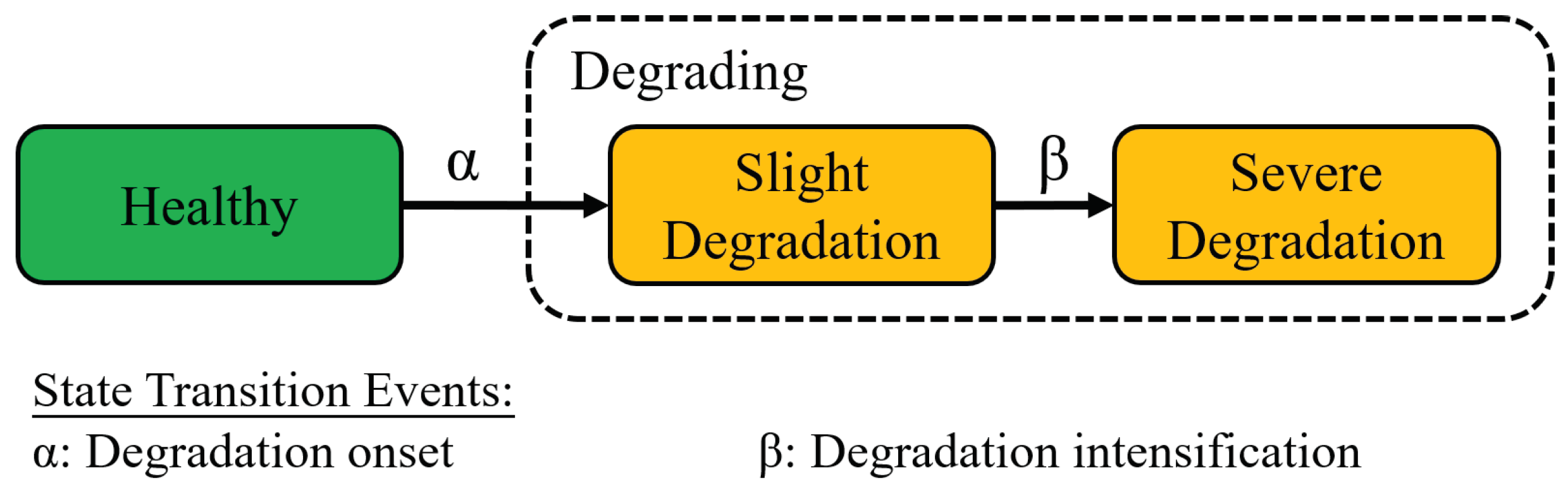
2.1. Health Model Structure

In the literature, bearing lifetime is commonly represented as a two-state process [19,20]. The first state is the Healthy state, characterized by steady-state behavior of bearing features, and the second state is the Degrading state, characterized by time-series trends in machine features that can be used to detect and track bearing deterioration [21]. However, the degradation of bearings can be complex, such that a single model is unable to track the entire process. So, this study augments the fundamental two-state bearing model by splitting the Degrading state into two sub-states, Slight Degradation and Severe Degradation, as shown in Figure 1. As described in later sections, the addition of a Slight Degradation state allows the health model to detect the presence of degradation, a valuable warning flag for system operators, even before the degradation process has progressed far enough to make reliable TTF predictions.

The steady-state descriptor presented by previous approaches is carried over here to describe bearing behavior in the Healthy state. We make the assumption that the distributions of machine features in the Healthy state are approximately normal within a bounded range of a normal mean. When a degradation onset event ($\alpha$) occurs, this means the bearing is about to degrade. The detection of a degradation onset event triggers the bearing to enter the Slight Degradation state. Generally, the Slight Degradation state is characterized by a departure from steady-state behavior and the emergence of time-series trends in one or more features. Within this study, a linear model is used to track slight degradation.

Following this state, a degradation intensification event ($\beta$) can be detected, at which point the degradation process is accelerated such that the model used in the Slight Degradation state can no longer describe the bearing’s degradation. At this point, the bearing enters the Severe Degradation state. In this state, the degradation process has progressed enough that it becomes possible to make reliable TTF predictions using a new degradation model. An exponential model is used here to track severe degradation, a choice that is supported by previous studies on bearing degradation [17,18,22].

The failure prediction process proposed by this work is illustrated in Figure 2. All components necessary to predict the TTF distribution of a bearing are included in an entity called a multi-state model $\left(M\right)$. A multi-state health-model consists of a model for degradation onset detection $\left(Q_{\alpha }\right)$, a model for degradation intensification $\left(Q_{\beta }\right)$, and a failure time predictor model $\left(P\right)$. Each of these components are described later sections, and can be written as functions of their model parameters, as in Figure 2.

2.2. Detection of Degradation Onset

The proposed method uses a combination of machine features as the multivariate detection health index $I_D=(i_1,i_2,\cdots i_m)$ to detect the occurrence of the degradation onset event $\left(\alpha \right)$ for each bearing. The features chosen here should show dynamic behaviors when in the early stage of bearing degradation, deviating from the uniform behavior in Healthy state. The method for $\alpha$ detection consists of the detection based on each individual feature $i_d$ ($d\in \mathbb{Z},1\le d\le m$), which is normalized independently. The $\alpha$ detection begins with a window of n feature values, where the mean of these n values in the window $\left(X\right)$ is computed. Meanwhile, the mean $\left(a\right)$ and the standard deviation $\left(\sigma \right)$ of all of the measured values are computed. As the window moves, the mean value over the window $\left(\overline{X}\right)$ is continuously compared to the historical mean $\left(a\right)$. Based on the assumption that all the features included in $I_D$ follow normal distributions in the Healthy state, approximately 99.7% of the data points should lie within three standard deviations of the mean. So we set the threshold to $a\pm 3\sigma$. Thus, if

$$|\overline{X}-a|>3\sigma ,$$

(1)

then a candidate degradation onset is detected. If a candidate degradation onset is detected in all of the features $i_d\in I_D$, then $\alpha$ is detected and the bearing should transition to Slight Degradation state. Alternatively, other $\alpha$ detection criteria, such as a majority of features crossing the threshold, can also be used in different system contexts.

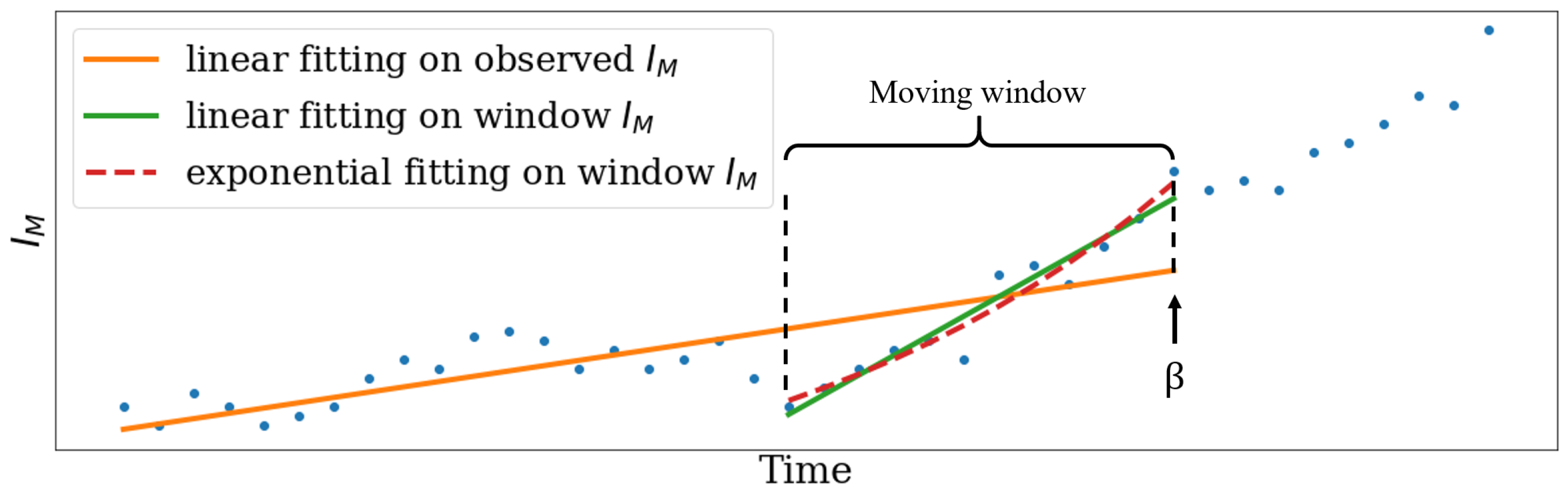
2.3. Detection of Degradation Intensification

Once a bearing enters a Slight Degradation state, a univariate prognostic health index $I_M$ is used to track degradation. The physical quantity represented by $I_M$ can vary based on the bearing and the monitoring system’s sensing capabilities. For example, this index may track the internal bearing temperature or the power present in a particular vibration frequency band. So, knowledge from system experts should be relied upon to select an index that reliably indicates system degradation. Automated processes for health index selection proposed in recent literature can also be utilized [23,24].

The approach for degradation intensification $\left(\beta \right)$ detection begins with a window of N prognostic health index values. The moving window is updated once a new data point is observed. In each iteration, a least squares linear regression and an exponential regression are performed over the window. Additionally, a linear regression model is fitted to all of the observed data. An example of the expected behavior of three regressions during the detection of $\beta$ is shown in Figure 3. The R-squared ($R^2$) values are computed for each regression model. The $R^2$ thresholds ${\gamma }_0$, ${\gamma }_1$, and ${\gamma }_2$ are predefined for the linear regression on the window data, exponential regression on window data and the linear regression on all of the observed data, respectively. Usually, these thresholds are initially determined from historical instances. The condition that represents the detection of $\beta$ is given by

$$\left\{\begin{array}{c}{R}_0^2<{\gamma }_0\hfill \\ R_1^2>{\gamma }_1\hfill \\ R_2^2<{\gamma }_2\hfill \end{array}\right.$$

(2)

where $R_0^2$, $R_1^2$, and $R_2^2$ are the R-squared values for the linear regression on window data, exponential regression on window data, and the linear regression on all observed data. The first instance when all these regression values violate their respective thresholds simultaneously indicates the time of degradation intensification $\left(\beta \right)$.

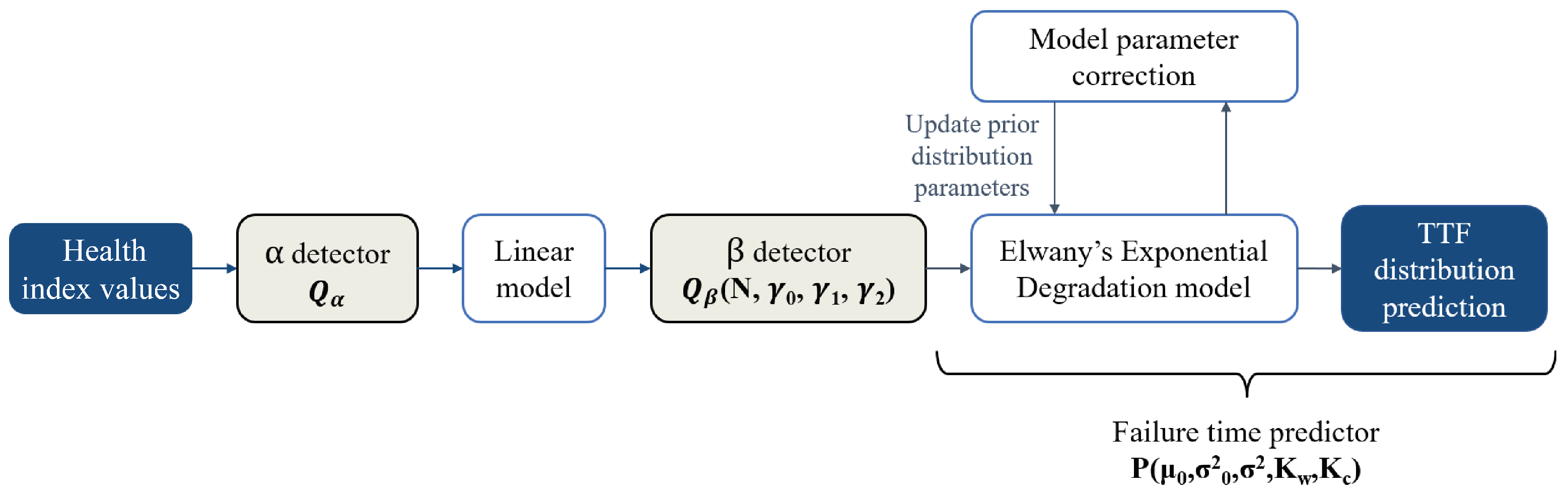
2.4. Prediction of TTF Distribution with Bayesian Updating Method

Once degradation intensification $\left(\beta \right)$ is detected, the bearing is assumed to be in the Severe Degradation state, for which an exponential random coefficient model is applied to predict the distribution of TTF. The method described here treats slight degradation and severe degradation as separate processes with distinct trend models. So, only prognostic health index values measured after degradation intensification are used to fit the exponential severe degradation model. The similarity between a linear trend and an early exponential trend suggests that it may be reasonable to the view slight degradation stage as the beginning of a single exponential degradation process. However, our analysis of several bearing failure instances has shown that segmenting the degradation process results in more accurate TTF predictions.

2.4.1. Exponential Random Coefficient Model

Random coefficient models are often used to describe stochastic degradation processes by adding random coefficients into degradation models [25]. When online measurements are available to track the process being modeled, the distributions of the random coefficients can be adapted using a Bayesian update rule, as in [17]. In [18], linear and exponential random coefficient models with error terms that follow Brownian motion were proposed and the mean remaining life was used for TTF estimation. We extend the random coefficient model from these works and incorporate it into the proposed multi-state health model.

For simplicity of computation, we assume the exponential curve passes through the last data point of the linear curve in the Slight Degradation state to fix the offset (b) of the exponential model. The exponential random coefficient model with one parameter can be written in the form

$$S\left(t_k\right)=\varphi ·e^{\theta t_k+\epsilon \left(t_k\right)}+b,$$

(3)

where $S\left(t_k\right)$ is the value of the prognostic health index $I_M$ at time $t_k$, $\varphi$ is a constant deterministic parameter, $\theta$ is a random variable coefficient assumed to follow a normal distribution $\left(\pi \right(\theta \left)\right)$ with mean ${\mu }_0$ and variance ${\sigma }_0^2$, b is the fixed offset determined by the linear Slight Degradation model, and $\epsilon \left(t_k\right)$ is an error term following a Brownian motion with mean zero and variance parameter ${\sigma }^2$. For mathematical convenience, we take the logarithm of $S\left(t_k\right)$. Then the model can be written as follows:

$$L\left(t_k\right)=ln(S\left(t_k\right)-b)={\varphi }^{\prime }+\theta t_k+\epsilon \left(t_k\right),$$

(4)

where $L\left(t_k\right)$ is the logarithm of $S\left(t_k\right)$ and ${\varphi }^{\prime }=ln\left(\varphi \right)$.

2.4.2. Bayesian Updating of the Distribution Parameters

A Bayesian update method is used to adapt the exponential model parameter $\theta$ when new measurements of the prognostic health index are made. With this approach, the prior distribution of the model parameter is updated based on a new measurement, resulting in a posterior distribution that becomes the prior for the next measurement. A method for defining a prior distribution before any measurements have been made is presented in Section 3.

Equations to compute the posterior distribution parameters are derived in [18] and defined by (5) and (6).

$$\begin{array}{cc}\hfill {\mu }_{\theta ,t_k}& =\frac{{\mu }_0{\sigma }^2+\left(L\left(t_k\right)-{\varphi }^{\prime }\right){\sigma }_0^2}{t_k{\sigma }_0^2+{\sigma }^2}\hfill \end{array}$$

(5)

$$\begin{array}{cc}\hfill {\sigma }_{\theta ,t_k}^2& =\frac{{\sigma }^2{\sigma }_0^2}{t_k{\sigma }_0^2+{\sigma }^2}\hfill \end{array}$$

(6)

One limitation of this update method, however, is that the closed-form solutions in (5) and (6) force the exponential model to weigh each historical data point equally, thus making the exponential curve emphasize early data and fail to capture the rapid increase when the TTF becomes smal. In order to solve this problem, our proposed method introduces a correction term to adjust ${\mu }_{\theta ,t_k}$ before using it to update the prior distribution for the next prediction. The error correction process can make the model more adaptive to the rising trends of actual data, and improve the accuracy of the TTF estimation.

To correct the posterior mean for $\theta$ at time $t_k$, an error term is defined, as shown in (7), as the sum of the weighted difference between actual and predicted $I_M$ from the beginning of the Severe Degradation state to time $t_k$, when the most recent data is observed.

$$e(t_k)=\sum _{i=1}^{k}w(K_w,t_i)·(s(t_i)-\tilde{S}(t_i))$$

(7)

In (7), $e\left(t_k\right)$ is an error term for the correction of ${\mu }_{\theta ,t_k}$ at time $t_k$, $s\left(t_i\right)$ is the actual $I_M$ at $t_i$, $\tilde{S}\left(t_i\right)$ is the predicted $I_M$ calculated as $\tilde{S}\left(t_i\right)=\varphi ·exp({\mu }_{\theta ,t_k}·t_k)+b$, and $w(K_w,t_i)$ is an exponential weighting term, $w(K_w,t_i)=(1-K_w)K_w^{k-i}$. A correction term is given as

$$\Delta \theta \left(t_k\right)=K_c·e\left(t_k\right),$$

(8)

where $K_c$ is a constant correction gain. Now, the value we use to update the mean of the model parameter $\theta$ in the prior distribution for the next prediction is

$${\mu }_{\theta ,t_k}^{\prime }={\mu }_{\theta ,t_k}+\Delta \theta \left(t_k\right).$$

(9)

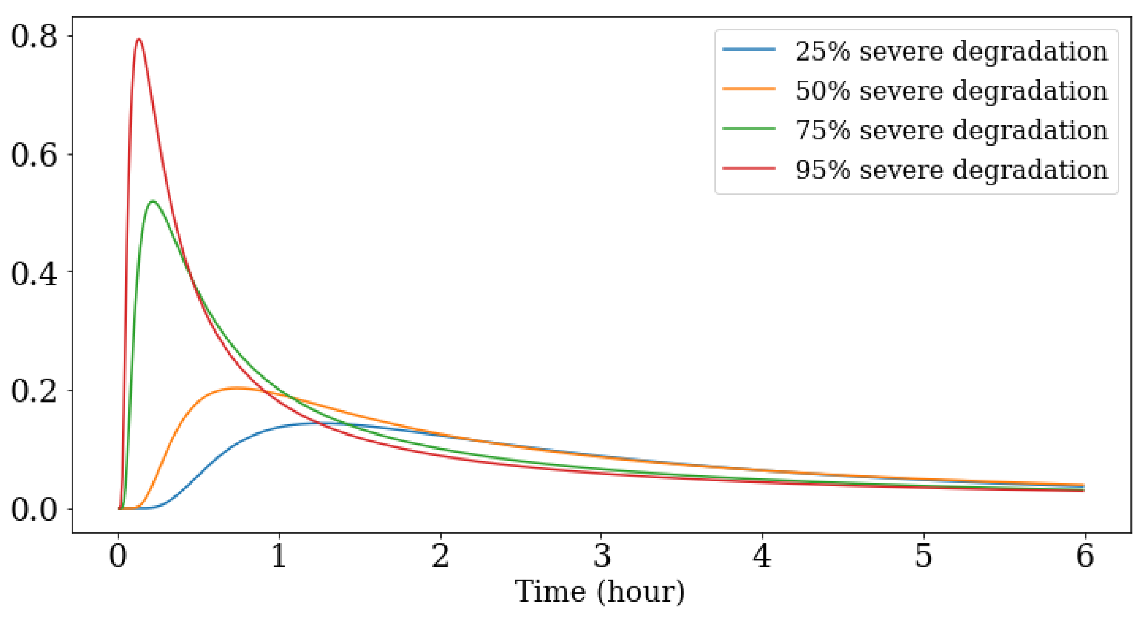
2.4.3. Computing the TTF Distribution

Having computed the posterior distribution of $\theta$ at time $t_k$, we would now like to determine the distribution of the TTF of the monitored bearing. For this purpose, we need to find a predefined failure threshold $\delta$ for the prognostic health index $I_M$. In general, such failure thresholds are not always clearly defined and are mostly unavailable in on-line analysis, so estimating one for a given application requires knowledge of industrial standards, application precision and engineering judgment [17]. The following method is extended from the approach in [18].

Give the failure threshold $\delta$ and a time $t_k$, we define the random variable $L(t_k+t)$ as the logged value of $I_M$ observed after t time units, $t>0$. Given $L\left(t_1\right),\cdots ,L\left(t_k\right)$ observed at times $t_1,\cdots ,t_k$, the mean and variance of $L(t_k+t)$ are given as

$$\tilde{\mu }\left(t_k+t\right)={\mu }_{\theta ,t_k}t+L\left(t_k\right)$$

(10)

$${\tilde{\sigma }}^2\left(t_k+t\right)={\sigma }_{\theta ,t_k}^2{t}^2+{\sigma }^{2}t.$$

(11)

Next, we define a random variable T to be the remaining life of a partially degraded bearing such that $L(t_k+T)=\delta$. Then the conditional cumulative distribution function (cdf) of T given $L\left(t_1\right),\cdots ,L\left(t_k\right)$ can be computed as follows:

$$P(T\le t|L\left(t_1\right),\cdots ,L\left(t_k\right))=\Phi \left(\frac{\tilde{\mu }\left(t+t_k\right)-\delta }{\tilde{\sigma }\left(t+t_k\right)}\right),$$

(12)

where $\Phi (·)$ is the cdf of a standard normal random variable. Now, we have shown how to find the conditional cdf of the remaining life of a bearing at time $t_k$. We can easily find the cdf of the TTF by adding current time $t_k$ to the remaining life. This procedure for Bayesian updating of prior distribution parameters and estimation of the TTF distribution is performed every time a new prognostic health index $I_M$ is observed by the model.

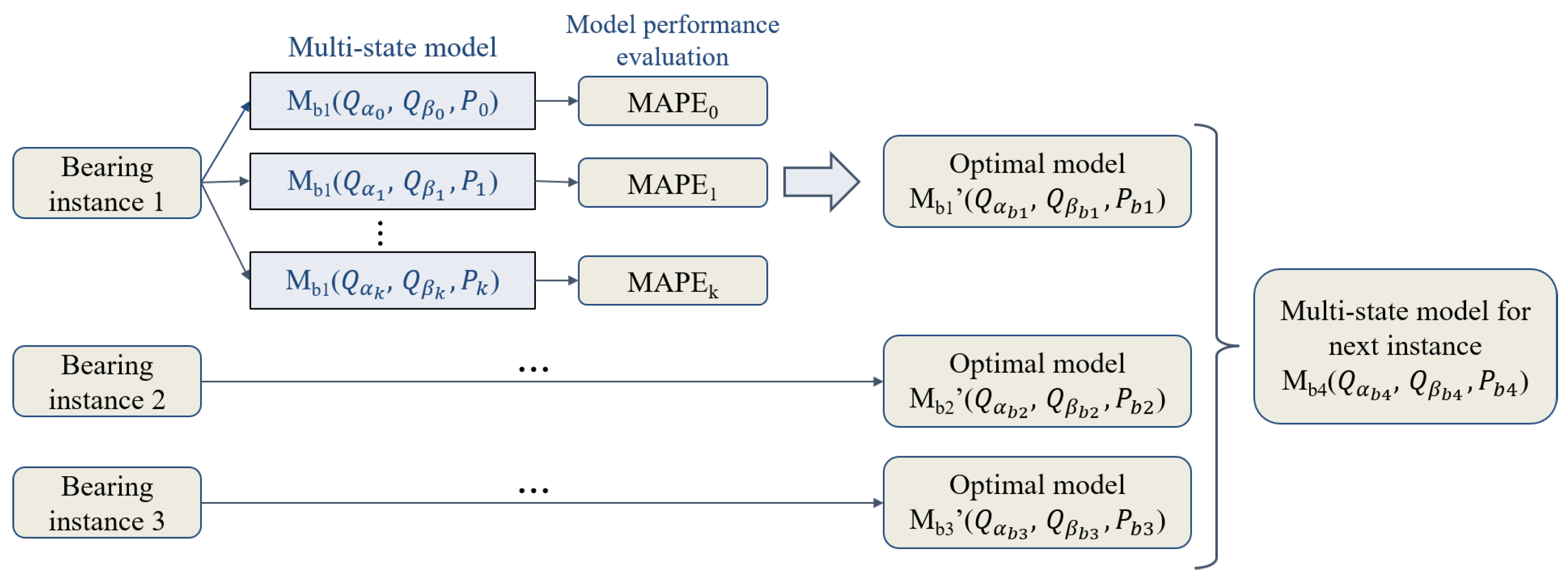
3. Model Training Process

This section presents the training process of the multi-state health model described in Section 2. This process makes the model more adaptive to a wide range of bearing instances in the same system. During a continuous manufacturing process, a well-suited health model for operating equipment should be adjustable when new condition data is observed. It is helpful to consider this training process in the context of an example equipment lifetime, shown in Figure 4. A multi-state health model generated from scratch (or from historical data if available) detects a degradation onset event on a bearing component, and triggers a transition from the Healthy state to the Degrading super-state. Next, based on the TTF prediction provided by the proposed model during the Severe Degradation state, an equipment shutdown is prompted for repair. After that, the equipment is brought back to a Healthy state, and the training method generates a new health model based on previous model and last failure instance. The newly generated model detects state transition points and predicts the TTF distribution until a repair event happens. In other words, with the application of the training method, the proposed health model is updated once a new failure instance is encountered.

The remainder of the section first describes the evaluation metrics that are used to evaluate the performance of generated models in the training process. Next, we elaborate on the training method that enables the proposed model to be adjustable when new failure instances are encountered.

3.1. Evaluation Metrics

This section presents the metrics that are used to evaluate the model performance. For each prediction of TTF made at time $t_k$, a percentage prediction error is computed as follows:

$$D_k=\frac{|T_{\delta }-{\widehat{T}}_{t_k}|}{T_{\delta }}\times 100\%.$$

(13)

where $T_{\delta }$ is the actual TTF and ${\widehat{T}}_{t_k}$ is the TTF predicted at time $t_k$.

For further evaluation of the TTF distribution, we calculate an approximate 90th Percentile Interval (PI), $(a_k,b_k)$, for the predicted TTF $T_k$ at each given time $t_k$. We let $a_k$ denote the 5th percentile and $b_k$ denote the 95th percentile of the TTF distribution. The calculation of $a_k$ and $b_k$ uses the following expressions:

$$P(T_k\le a_k\mid S\left(t_1\right),S\left(t_2\right),\cdots ,S\left(t_k\right))=0.05$$

(14)

$$P(T_k\le b_k\mid S\left(t_1\right),S\left(t_2\right),\cdots ,S\left(t_k\right))=0.95.$$

(15)

A higher accuracy metric would involve the conversion to a logarithm chart, but it would be more complicated. Given the sparsity of data, we use the approach described above for simplicity.

Moreover, in order to evaluate the performance of a model over the whole degradation process of a bearing, we use an evaluation metric from [26] called mean absolute percentage error (MAPE) which is given by

$$\mathrm{MAPE}=(\sum _{k=1}^T\frac{|T_{\delta }-{\widehat{T}}_{t_k}|}{T_{\delta }}\times 100\%)/T.$$

(16)

A multi-state health model that makes more accurate TTF predictions over a long period has a lower MAPE value. This metric is used for single failure model evaluation in the following training process.

3.2. Training Method

In this section, we describe a training framework used across multiple bearing instances between repair events in the same system. Initially, when the model has not seen any bearing instances before, we generate a model with all the parameters shown in Figure 2 randomly generated for on-line analysis on the first bearing instance and use the MAPE value to evaluate the model. In the testing done for this study, parameters N and ${\mu }_0$ were generated by sampling from a uniform distribution with bounds $[0,10]$, and parameters ${\gamma }_0,{\gamma }_1,{\gamma }_2,{\sigma }_0^2$ and ${\sigma }^2$ were generated by sampling from a uniform distribution with bounds $[0,1]$. Using these prior distributions resulted in models with reasonable failure prediction here, but may need to be adjusted for other systems. Once the first bearing has failed, we can undergo a training process within this single bearing in order to learn an optimal set of model parameters for it. After that, if we need to do another on-line analysis on a new bearing instance, then we can apply the optimal model obtained from the first bearing to the new bearing. Due to the assumption that all the bearings are operating in the same system, there should be some common patterns in the bearing degradation process. Therefore, we suppose that a model that provides accurate predictions on historical bearing instances will also work well on subsequent bearing instances.

Figure 5 shows an example of the model training process. At this point in the training process, three bearing failure instances have been encountered, and our model uses this historical data to train a revised model for the next instance.

For a single known bearing instance, k multi-state models, expressed as

$$M(Q_{\alpha },Q_{{\beta }_0},P_0),M(Q_{\alpha },Q_{{\beta }_1},P_1),\cdots ,M(Q_{\alpha },Q_{{\beta }_k},P_k),$$

with different parameters for $\beta$, detector $Q_{\beta }$, and TTF predictor P will be generated. In our implementation, the window size N, the $R^2$ thresholds ${\gamma }_0$, ${\gamma }_1$, ${\gamma }_2$, the mean ${\mu }_0$ and variance ${\sigma }_0^2$ for the prior distribution of $\theta$, and the variance ${\sigma }^2$ for the distribution of the error term $\epsilon \left(t_k\right)$ are randomly generated for each model. In this analysis, the weighting parameter $\left(K_w\right)$ and correction gain $\left(K_c\right)$ constants are set to $K_w=0.8$ and $K_c=0.1$. These values establish an appropriate balance between trusting historical observations and adapting to new observations in this analysis, but can be modified for other systems. If the time of degradation intensification $\left(\beta \right)$ is detected too close to the actual TTF, there is too little time left to obtain prediction results and schedule a repair event. Thus, we set a threshold that if $\beta$ is detected less than 5 h before the TTF, then that model will be discarded because the time left is too little for operators to schedule maintenance work before bearing failure. We compare the MAPE values for all of the remaining models, and choose the one that minimizes the MAPE value as the optimal model $M^{\prime }(Q_{\alpha },Q_{\beta },P)$ for this bearing instance. Indeed, a more intelligent gradient descent algorithm could be used here so that we can find the optimal model with the lowest MAPE in a step-wise procedure.

Once a bearing instance or several bearing instances are known, a multi-state health model can be trained with these instances. Since each known bearing instance is paired with an optimal model, we take the average of the learned model parameters $(N,{\gamma }_0,{\gamma }_1,{\gamma }_2,{\mu }_0,{\sigma }_0^2,{\sigma }^2)$ to construct a model that is used for online testing with new bearings.

4. Case Study

In this section, we describe how the proposed multi-state health model and training process is implemented to analyze the bearing run-to-failure dataset provided by the Center for Intelligent Maintenance Systems (IMS) [27] and discuss the results of the model training experiments.

4.1. IMS Dataset

The proposed method is tested on the IMS bearing data. Four Rexnord ZA-2115 double row bearings are installed on the shaft and High Sensitivity Quartz ICP accelerometers are installed on the bearing housing. An AC motor is coupled to the shaft to keep the rotation speed constant at 2000 RPM and a radial load of 6000 lbs is applied onto the shaft and bearings by a spring mechanism. The data packet includes the vibration data of four bearings in the test system through three test-to-failure experiments. Each data set that corresponds to each test consists of individual files that are 1-s vibration signal snapshots recorded every 10 min. Each file consists of 20,480 points with the sampling rate set at 20 kHz. These data are recorded every 10 min (except the first 43 files for test 1 are taken every 5 min).

4.2. Model Implementation

To detect degradation onset in this dataset, a combination of kurtosis, skewness, peak frequency, and peak-to-peak features, defined in

Table 1. Statistic feature expressions.

Feature	Expression
Kurtosis	$\frac{1}{N}{\sum }_{i=1}^N\frac{{(x_i-\overline{x})}^4}{{\sigma }^4}$
Skewness	$\frac{1}{N}{\sum }_{i=1}^N\frac{{(x_i-\overline{x})}^3}{{\sigma }^3}$
Peak Frequency	$max\left(f\right)$
Peak-to-peak	$x_{max}-x_{min}$
Root Mean Square (RMS)	${\left(\frac{1}{N}{\sum }_{i=1}^N{x}_i^2\right)}^{\frac{1}{2}}$

was used as the multivariate detection health index $I_D$. The root mean square (RMS) feature, as defined in Table 1, was selected as the univariate prognostic health index $I_M$ for the detection of degradation intensification $\left(\beta \right)$ and the prediction of TTF distribution. In order to obtain a fixed failure threshold value $\delta$, we perform an ordinary linear regression on the last 10 data points before failure, and take the last value from the linear model as $\delta$.

We first applied the proposed model to a single bearing, bearing 3 in test 3 of the IMS dataset, to observe how the TTF distribution changes as more data are given to the model. The model parameters are fine-tuned after several off-line tests. The bottom plot in Figure 6 shows the two-stage degradation regression model fit to this bearing’s prognostic health index $I_M$. The predicted trajectory for $I_M$ in the Slight Degradation state is generated by a linear model, while that for $I_M$ in the Severe Degradation state is generated by an exponential model. We find that the bearing’s prognostic health index $I_M$ closely follows the degradation trajectories predicted by the proposed model and that the exponential model reaches the failure threshold at approximately the same time as the $I_M$ measurements. This behavior supports the decision to model bearing degradation as a two-stage process with linear and exponential trajectories. For comparison, the top plot in Figure 6 shows the exponential regression model that would be generated if bearing degradation was treated as a single-stage process. This plot shows close agreement between the exponential model and early $I_M$ measurements, but the exponential model does not adapt to the increased rate of bearing degradation later in the test. As a result, the exponential model reaches the failure threshold significantly after the $I_M$ measurements, leading to inaccurate TTF predictions.

Figure 7 shows the probability density function (PDF) of TTF at different degrees of degradation. The bearing is at 0% severe degradation the instant that degradation intensification $\left(\beta \right)$ is detected, and at 100% severe degradation the instant that it fails. As time passes, the peak of the PDF approaches zero hours, indicating that TTF predictions become smaller as the degradation progresses. Furthermore, the peak value of the PDF becomes larger as time passes, indicating that TTF can be predicted with higher confidence.

Table 2. TTF prediction results on bearing 3 in test 3 in the IMS dataset.

Time (Hour)	% Severe Degradation Time	Actual Failure Time (Hour)	Predicted Failure Time (Hour)	5th Percentile	95th Percentile	% Error D
26.0	25%	30.5	33.02	25.60	>100	8.25%
27.5	50%	30.5	31.31	25.25	>100	2.64%
29.0	75%	30.5	30.96	24.86	76.06	1.50%
30.2	95%	30.5	31.02	24.79	63.69	1.69%

illustrates the prediction results on bearing 3 in test 3 at $25\%$, $50\%$, $75\%$, and $95\%$ percentage of the severe degradation time. At each listed prediction time, the predicted TTF, an approximate 90th percentile interval, and a percentage prediction error D are computed and shown in the table. As more degradation data is seen by the model, the predicted TTF approaches the true TTF. The range of the 90th percentile interval also becomes smaller, illustrating that model prediction becomes more confident.

4.3. Results

To test the effectiveness of the proposed model training process, we set up a training and testing sequence using the IMS dataset. The bearings in this dataset encountered multiple failure modes, each characterized by surface defects at different internal bearing surfaces. An inner race defect occurred in bearing 3 in test 1, outer race defects occurred in bearing 3 in test 3 and bearing 1 in test 2, and a rolling element defect occurred in bearing 4 in test 1. Bearing 3 in test 3 and bearings 3 and 4 in test 1 are used for training sequentially. Bearing 1 in test 2 is treated as a test bearing for the purposes of evaluating the proposed training process. In

Table 3. Model training results.

Model	Bearing	MAPE 1
Randomly generated	Test 3 Bearing 3	16.637%
Optimal model among 50 randomly generated models	Test 3 Bearing 3	4.594%
Randomly generated	Test 2 Bearing 1	5.962%
Model trained with Test 3 Bearing 3		3.792%
Model trained with Test 3 Bearing 3 and Test 1 Bearing 3		5.483%
Model trained with Test 3 Bearing 3, Test 1 Bearings 3 & 4		5.156%

¹ The MAPE value for a randomly generated model is an average MAPE of all valid models from the 50 randomly generated ones.

, we compare the performance of a randomly generated model and an optimal model for a single bearing in the upper part, and compare the performance of the models with different knowledge of historical bearing failures on the testing bearing in the lower part.

Comparing the two models in the upper part of Table 3, the MAPE score of the optimal model for bearing 3 in test 3 is much smaller than that of the randomly generated model, indicating that the training method within a single bearing results in more accurate TTF predictions. Additionally, a comparison of the randomly generated model for bearing 1 in test 2 with the models trained on data from historical bearing failures shows that all trained models result in a lower MAPE score than the randomly generated model. This indicates that the proposed training process helps to increase TTF prediction accuracy for new failures. It is notable that these improvements in prediction accuracy are achieved across tests with different failure modes. This underscores the general nature of this training process, making it suitable to learn and make predictions across different bearing failure modes. The training approach takes only a few seconds to determine the optimal model for test bearings, making it suitable for online TTF prediction. The IMS bearing dataset contains a limited number of bearing failures, so it is difficult to determine whether a larger number of historical failure instances would improve prediction accuracy further.

5. Conclusions

In this paper, a multi-state health model is proposed to predict the TTF distribution of rolling element bearings on rotating equipment. Given historical data of bearing failure, this approach employs a regression-based method to detect degradation state transition points, and applies an exponential random coefficient model to predict a TTF distribution. A model training framework is introduced to make our proposed model adjustable to unseen bearing instances in the same system. A case study demonstrates that the proposed method provides accurate TTF predictions across multiple bearing failures. The training method enables the health model to be adaptive to condition changes in the system, especially when new failure instances are obtained after a rotating equipment gets repaired, and reduces the time for generating a reliable model for an unknown bearing instance. Therefore, the proposed approach is a compelling solution to the problem of online bearing prognosis.

Future improvement can be done to develop a more efficient parameter search algorithm, which will be able to narrow down the search space of the adjustable model parameters as more failures are observed. An efficient parameter search algorithm would reduce the time to find an optimal model for a single run-to-failure bearing instance. Moreover, since the IMS bearing data contains a limited number of bearings that failed during run-to-failure experiments, averaging the learned model parameters in the model training framework can satisfy the need to generate a proper model for future failures in the system. Future work could be done to determine and separate the common and varying aspects of the model if more failure instances are available. The methods proposed here were effective at making failure predictions for bearing failures induced by natural friction between the bearing components. However, other mechanisms, such is improper lubrication and contaminating particles, can also induce failure, and further testing is necessary to validate these methods with those failure modes (which were not introduced in the experiments used for this work). The multi-state health model and training process proposed here should also be applied to other systems that exhibit exponential degradation.

References

1. Jiang, J.; Zhang, B. Rolling element bearing vibration modeling with applications to health monitoring. J. Vib. Control 2012, 18, 1768–1776. [Google Scholar] [CrossRef]
2. Nandi, S.; Toliyat, H.A.; Li, X. Condition Monitoring and Fault Diagnosis of Electrical Motors, A Review. IEEE Trans. Energy Convers. 2005, 20, 719–729. [Google Scholar] [CrossRef]
3. Li, Y.; Billington, S.; Zhang, C.; Kurfess, T.; Danyluk, S.; Liang, S. Adaptive prognostics for rolling element bearing condition. Mech. Syst. Signal Process. 1999, 13, 103–113. [Google Scholar] [CrossRef]
4. Qiu, J.; Zhang, C.; Seth, B.B.; Liang, S.Y. Damage mechanics approach for bearing lifetime prognostics. Mech. Syst. Signal Process. 2002, 16, 817–829. [Google Scholar] [CrossRef]
5. Cubillo, A.; Perinpanayagam, S.; Esperon-Miguez, M. A review of physics-based models in prognostics: Application to gears and bearings of rotating machinery. Adv. Mech. Eng. 2016, 8, 1–21. [Google Scholar] [CrossRef] [Green Version]
6. Cerrada, M.; Sánchez, R.V.; Li, C.; Pacheco, F.; Cabrera, D.; Valente de Oliveira, J.; Vásquez, R.E. A review on data-driven fault severity assessment in rolling bearings. Mech. Syst. Signal Process. 2018, 99, 169–196. [Google Scholar] [CrossRef]
7. Neupane, D.; Seok, J. Bearing Fault Detection and Diagnosis Using Case Western Reserve University Dataset With Deep Learning Approaches: A Review. IEEE Access 2020, 8, 93155–93178. [Google Scholar] [CrossRef]
8. Peng, B.; Wan, S.; Bi, Y.; Xue, B.; Zhang, M. Automatic Feature Extraction and Construction Using Genetic Programming for Rotating Machinery Fault Diagnosis. IEEE Trans. Cybern. 2020, 51, 4909–4923. [Google Scholar] [CrossRef] [PubMed]
9. Qiu, H.; Lee, J.; Lin, J.; Yu, G. Wavelet filter-based weak signature detection and its application on rolling element bearing prognosis. J. Sound Vib. 2006, 289, 1066–1090. [Google Scholar] [CrossRef]
10. Ahmad, W.; Khan, S.A.; Kim, J.M. A Hybrid Prognostics Technique for Rolling Element Bearings Using Adaptive Predictive Models. IEEE Trans. Ind. Electron. 2018, 65, 1577–1584. [Google Scholar] [CrossRef]
11. Ali, J.B.; Chebel-Morello, B.; Saidi, L.; Malinowski, S.; Fnaiech, F. Accurate bearing remaining useful life prediction based on Weibull distribution and artificial neural network. Mech. Syst. Signal Process. 2015, 56–57, 150–172. [Google Scholar]
12. Mahamad, A.K.; Saon, S.; Hiyama, T. Predicting remaining useful life of rotating machinery based artificial neural network. Comput. Math. Appl. 2010, 60, 1078–1087. [Google Scholar] [CrossRef] [Green Version]
13. Cui, L.; Wang, X.; Xu, Y.; Jiang, H.; Zhou, J. A novel Switching Unscented Kalman Filter method for remaining useful life prediction of rolling bearing. Measurement 2019, 135, 678–684. [Google Scholar] [CrossRef]
14. Tobon-Mejia, D.A.; Medjaher, K.; Zerhouni, N.; Tripot, G. A Data-Driven Failure Prognostics Method Based on Mixture of Gaussians Hidden Markov Models. IEEE Trans. Reliab. 2012, 61, 491–503. [Google Scholar] [CrossRef] [Green Version]
15. Ren, L.; Sun, Y.; Cui, J.; Zhang, L. Bearing remaining useful life prediction based on deep autoencoder and deep neural networks. J. Manuf. Syst. 2018, 48, 71–77. [Google Scholar] [CrossRef]
16. Huang, C.G.; Huang, H.Z.; Li, Y.F.; Peng, W. A novel deep convolutional neural network-bootstrap integrated method for RUL prediction of rolling bearing. J. Manuf. Syst. 2021, 61, 757–772. [Google Scholar] [CrossRef]
17. Gebraeel, N.Z.; Lawley, M.A.; Li, R.; Ryan, J.K. Residual-life distributions from component degradation signals: A Bayesian approach. IIE Trans. 2005, 37, 543–557. [Google Scholar] [CrossRef]
18. Elwany, A.; Gebraeel, N. Real-Time Estimation of Mean Remaining Life Using Sensor-Based Degradation Models. J. Manuf. Sci. Eng. 2009, 131, 051005. [Google Scholar] [CrossRef]
19. Ginart, A.; Barlas, I.; Goldin, J.; Dorrity, J.L. Automated Feature Selection for Embeddable Prognostic and Health Monitoring (PHM) Architectures. In Proceedings of the 2006 IEEE Autotestcon, Anaheim, CA, USA, 18–21 September 2006; pp. 195–201. [Google Scholar]
20. Jin, X.; Sun, Y.; Que, Z.; Wang, Y.; Chow, T.W.S. Anomaly Detection and Fault Prognosis for Bearings. IEEE Trans. Instrum. Meas. 2016, 65, 2046–2054. [Google Scholar] [CrossRef]
21. Toothman, M.; Braun, B.; Bury, S.J.; Dessauer, M.; Henderson, K.; Wright, R.; Tilbury, D.M.; Moyne, J.; Barton, K. Trend-based repair quality assessment for industrial rotating equipment. IEEE Control Syst. Lett. 2020, 5, 1675–1680. [Google Scholar] [CrossRef]
22. Shao, Y.; Nezu, K. Prognosis of remaining bearing life using neural networks. Proc. Inst. Mech. Eng. Part I J. Syst. Control. Eng. 2000, 214, 217–230. [Google Scholar] [CrossRef]
23. Yang, F.; Habibullah, M.S.; Zhang, T.; Xu, Z.; Lim, P.; Nadarajan, S. Health Index-Based Prognostics for Remaining Useful Life Predictions in Electrical Machines. IEEE Trans. Ind. Electron. 2016, 63, 2633–2644. [Google Scholar] [CrossRef]
24. Liu, K.; Chehade, A.; Song, C. Optimize the Signal Quality of the Composite Health Index via Data Fusion for Degradation Modeling and Prognostic Analysis. IEEE Trans. Autom. Sci. Eng. 2017, 14, 1504–1514. [Google Scholar] [CrossRef]
25. Lei, Y.; Li, N.; Guo, L.; Li, N.; Yan, T.; Lin, J. Machinery health prognostics: A systematic review from data acquisition to RUL prediction. Mech. Syst. Signal Process. 2018, 104, 799–834. [Google Scholar] [CrossRef]
26. Coble, J.; Hines, J.W. Incorporating prior belief in the general path model: A comparison of information sources. Nucl. Eng. Technol. 2014, 46, 773–782. [Google Scholar] [CrossRef] [Green Version]
27. Lee, J.; Qiu, H.; Yu, G.; Lin, J.; Services, R.T. Bearing Data Set. Available online: https://ti.arc.nasa.gov/tech/dash/groups/pcoe/prognostic-data-repository/ (accessed on 19 November 2021).
Figure 1. Multi-state health model statechart.
Electronics 11 00257 g001
Figure 2. Framework of a multi-state health model M ( Q α , Q β , P ) .
Electronics 11 00257 g002
Figure 3. Detection of degradation intensification ( β ) .
Electronics 11 00257 g003
Figure 4. Example operating timeline.
Electronics 11 00257 g004
Figure 5. Framework of the training process. (given three observed bearing failure instances).
Electronics 11 00257 g005
Figure 6. I M degradation trajectories and regression models for single-stage degradation process (top) and 2-stage degradation process (bottom).
Electronics 11 00257 g006
Figure 7. PDF of remaining useful life at different percentage of bearing’s life.
Electronics 11 00257 g007