


Comparison of Grid Reactive Voltage Regulation with Reconfiguration Network for Electric Vehicle Penetration

Abstract
:1. Introduction
EV Charging Problem
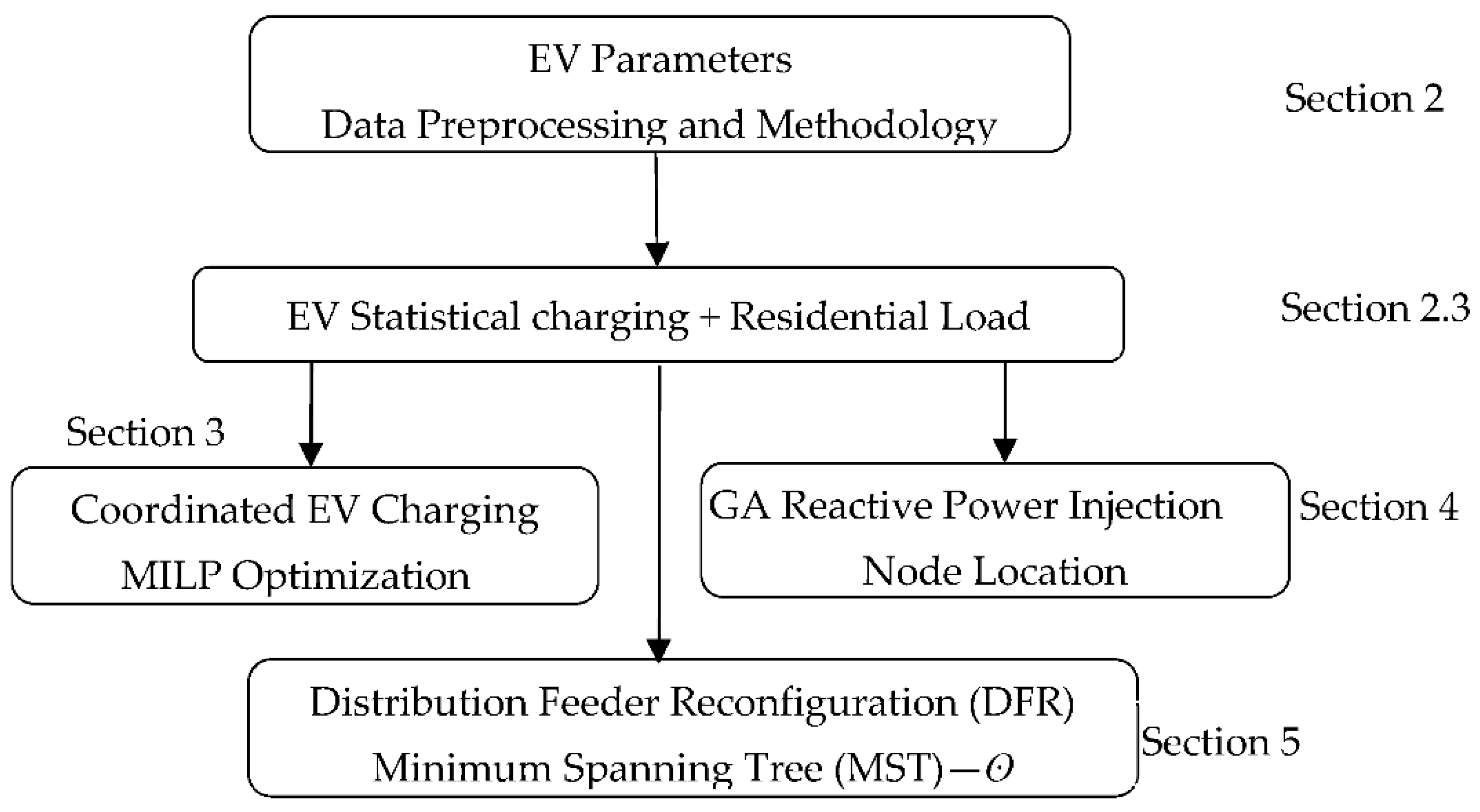
2. Simulation Methodology
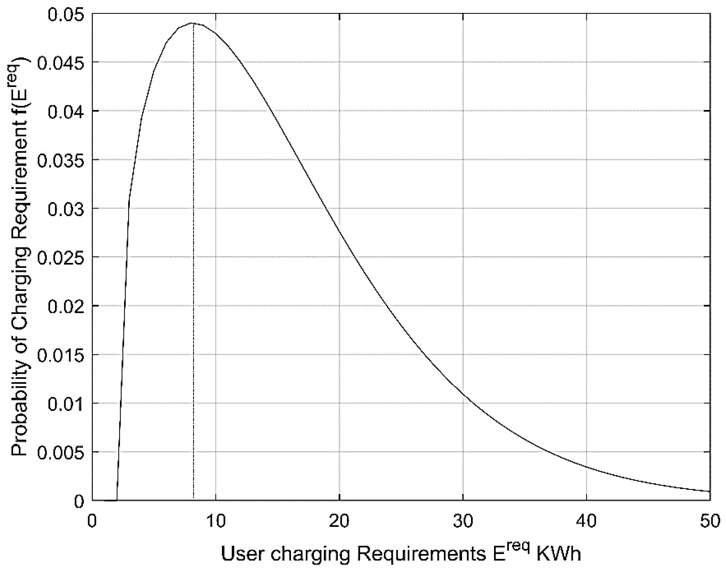
2.1. EV Charging Distribution
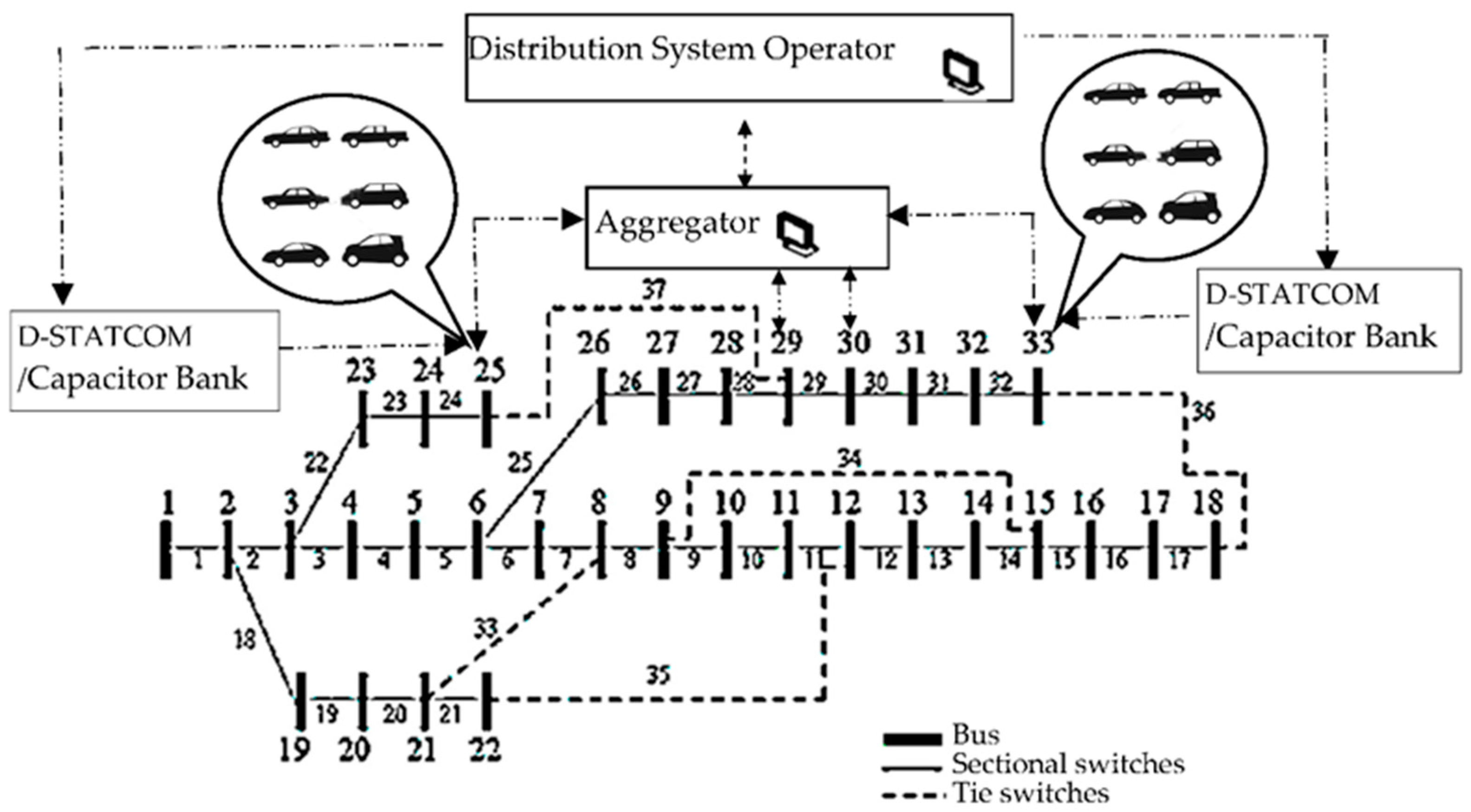
2.2. IEEE 33 Bus and EV Charging Parameters
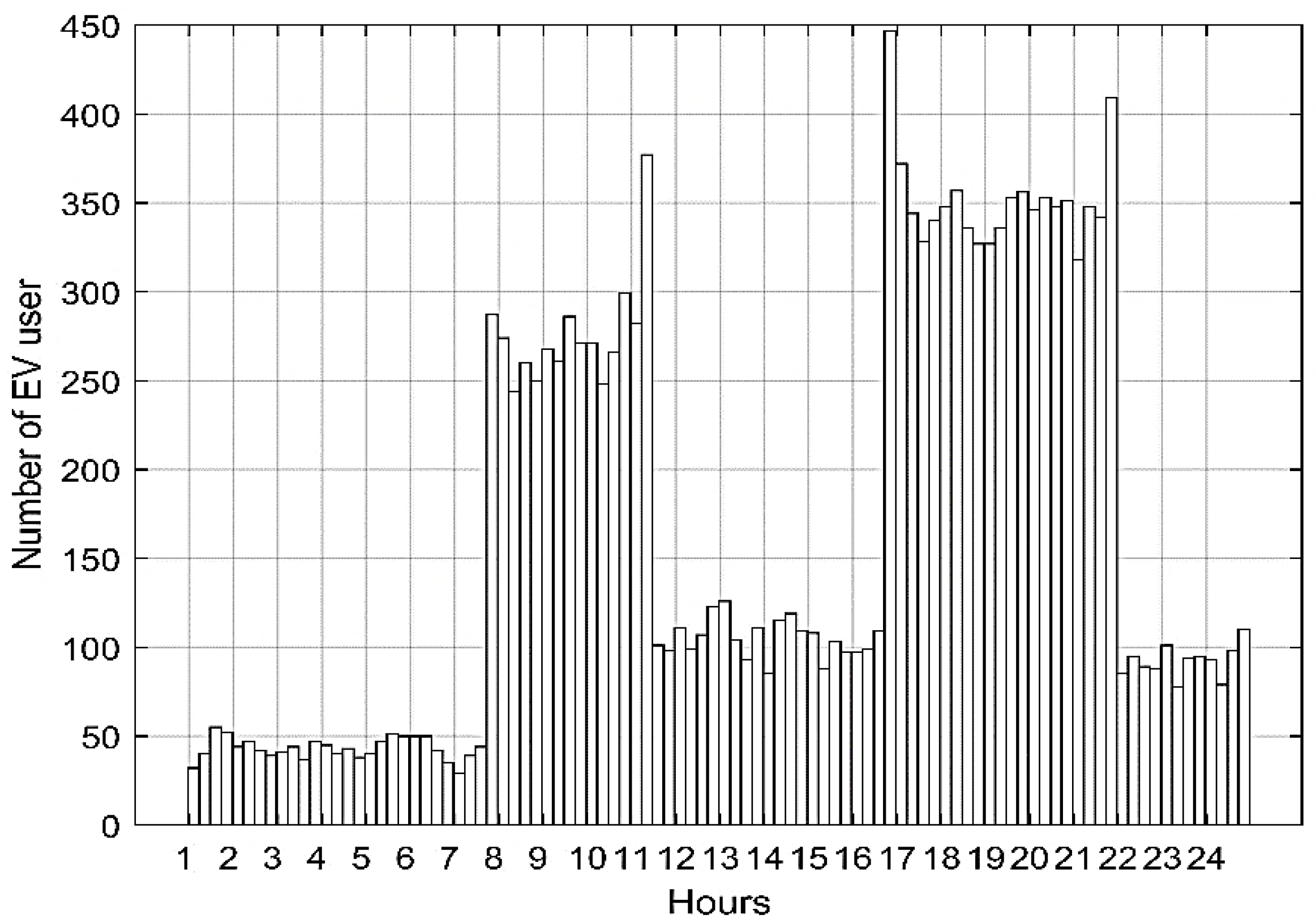
2.3. EV Charging Statistical Load
3. Coordinated EV Charging-MILP
3.1. Coordinated Power Flow Analysis
4. Power Injection GA-Optimization with Power Flow Analysis
4.1. Injection Power Flow Analysis
4.2. Random Search of Injection Nodes and Magnitude
4.3. Reactive Injection Objective Function
5. Minimum Spanning Tree (MST) Analysis
5.1. Branch Search for Maximum Flow
5.2. MST Power Flow Analysis
5.3. MST Objective Function
6. Results and Analysis
7. Conclusions
Author Contributions
Funding
Data Availability Statement
Conflicts of Interest
Appendix A

| No. | Sn | Rc | Resistance | Reactance |
|---|---|---|---|---|
| 1 | 1 | 2 | 0.0922 | 0.0470 |
| 2 | 2 | 3 | 0.4930 | 0.2511 |
| 3 | 3 | 4 | 0.3660 | 0.1864 |
| 3 | 3 | 4 | 0.3660 | 0.1864 |
| 4 | 4 | 5 | 0.3811 | 0.1941 |
| 4 | 5 | 6 | 0.8190 | 0.7070 |
| 6 | 6 | 7 | 0.1872 | 0.6188 |
| 7 | 7 | 8 | 0.7114 | 0.2351 |
| 8 | 8 | 9 | 1.0300 | 0.7400 |
| 9 | 9 | 10 | 1.0440 | 0.7400 |
| 10 | 10 | 11 | 0.1966 | 0.0650 |
| 11 | 11 | 12 | 0.3744 | 0.1238 |
| 12 | 12 | 13 | 1.4680 | 1.1550 |
| 13 | 13 | 14 | 0.5416 | 0.7129 |
| 14 | 14 | 15 | 0.5910 | 0.5260 |
| 15 | 15 | 16 | 0.7463 | 0.545 |
| 16 | 16 | 17 | 1.289 | 1.721 |
| 17 | 17 | 18 | 0.732 | 0.574 |
| 18 | 2 | 19 | 0.164 | 0.1565 |
| 19 | 19 | 20 | 1.5042 | 1.3554 |
| 20 | 20 | 21 | 0.4095 | 0.4784 |
| 21 | 21 | 22 | 0.7089 | 0.9373 |
| 22 | 3 | 23 | 0.4512 | 0.3083 |
| 23 | 23 | 24 | 0.898 | 0.7091 |
| 24 | 24 | 25 | 0.896 | 0.7011 |
| 25 | 6 | 26 | 0.203 | 0.1034 |
| 26 | 26 | 27 | 0.2842 | 0.1447 |
| 27 | 27 | 28 | 1.059 | 0.9337 |
| 28 | 28 | 29 | 0.8042 | 0.7006 |
| 29 | 29 | 30 | 0.5075 | 0.2585 |
| 30 | 30 | 31 | 0.9744 | 0.963 |
| 31 | 31 | 32 | 0.3105 | 0.3619 |
| 32 | 32 | 33 | 0.341 | 0.5302 |
| 33 | 8 | 21 | 2 | 2 |
| 34 | 9 | 15 | 2 | 2 |
| 35 | 22 | 12 | 2 | 2 |
| 36 | 18 | 33 | 2 | 2 |
| Bus | |VL||pu| | deg| |
|---|---|---|
| 2 | 0.997 | 0.015 |
| 3 | 0.9829 | 0.097 |
| 4 | 0.9754 | 0.163 |
| 5 | 0.968 | 0.23 |
| 6 | 0.9495 | 0.136 |
| 7 | 0.946 | −0.096 |
| 8 | 0.9323 | −0.249 |
| 9 | 0.926 | −0.324 |
| 10 | 0.9201 | −0.388 |
| 11 | 0.9192 | −0.38 |
| 12 | 0.9177 | −0.368 |
| 13 | 0.9115 | −0.462 |
| 14 | 0.9092 | −0.542 |
| 15 | 0.9078 | −0.58 |
| 16 | 0.9064 | −0.604 |
| 17 | 0.9044 | −0.683 |
| 18 | 0.9038 | −0.693 |
| 19 | 0.9965 | 0.004 |
| 20 | 0.9929 | −0.063 |
| 21 | 0.9922 | −0.083 |
| 22 | 0.9916 | −0.103 |
| 23 | 0.9793 | 0.066 |
| 24 | 0.9726 | −0.023 |
| 25 | 0.9693 | −0.067 |
| 26 | 0.9475 | 0.175 |
| 27 | 0.945 | 0.232 |
| 28 | 0.9335 | 0.315 |
| 29 | 0.9253 | 0.393 |
| 30 | 0.9218 | 0.498 |
| 31 | 0.9176 | 0.413 |
| 32 | 0.9167 | 0.39 |
| 33 | 0.9164 | 0.383 |
| 34 | - | - |
| 35 | - | - |
References
- Shibo, L. Research on Distribution Network Voltage Regulation Strategy Adapting to Distributed Power Supply Access. Master’s Thesis, Shandong University of Technology, Zibo, China, April 2013. [Google Scholar]
- Li, Y.W. Smart Grid and its Application. Adv. Mater. Res. 2014, 986–987, 533–536. [Google Scholar] [CrossRef]
- Kotenev, V.I.; Kochetkov, V.V.; Elkin, D.A. The Reactive Power Control of the Power System Load Node at the Voltage Instability of the Power Supply. In Proceedings of the 2017 International Siberian Conference on Control and Communications, SIBCON, Astana, Kazakhstan, 29–30 June 2017; pp. 3–6. [Google Scholar]
- Meng, Q.; Che, R.; Gao, S. Reactive Power and Voltage Optimization Control Strategy in Active Distribution Network Based on the Determination of the Key Nodes. In Proceedings of the 2017 2nd Asia Conference on Power and Electrical Engineering (ACPEE 2017), Shanghai, China, 24–26 March 2017. [Google Scholar]
- Zechun, H.; Mingming, Z. Optimal Reactive Power Compensation for Medium and Low Voltage Distribution Network Considering Multiple Load Levels. Trans. China Electrotech. Soc. 2010, 25, 167–172. [Google Scholar]
- Liu, C.; Zhang, Y. Confirmation of Reactive Power Compensation Node and Its Optimal Compensation Capacity. Power Syst. Technol. 2007, 31, 78–81. [Google Scholar]
- Singh, J.; Tiwari, R. Electric Vehicles Reactive Power Management and Reconfiguration of Distribution System to Minimize Losses. IET Gener. Transm. Distrib. 2020, 14, 6285–6293. [Google Scholar] [CrossRef]
- Baran, M.E.; Wu, F.F. Network Reconfiguration in Distribution Systems for Loss Reduction and Load Balancing. IEEE Power Eng. Rev. 1989, 9, 101–102. [Google Scholar] [CrossRef]
- Zhang, C.-X.; Zeng, Y. Voltage and Reactive Power Control Method for Distribution Grid. In Proceedings of the 2013 IEEE PES Asia-Pacific Power and Energy Engineering Conference (APPEEC), Hong Kong, China, 8–11 December 2013. [Google Scholar]
- Rostami, M.-A.; Kavousi-Fard, A.; Niknam, T. Expected Cost Minimization of Smart Grids with Plug-In Hybrid Electric Vehicles Using Optimal Distribution Feeder Reconfiguration. IEEE Trans. Ind. Inform. 2015, 11, 388–397. [Google Scholar] [CrossRef]
- Cui, H.; Li, F.; Fang, X.; Long, R. Distribution Network Reconfiguration with Aggregated Electric Vehicle Charging Strategy. In Proceedings of the 2015 IEEE Power & Energy Society General Meeting, Denver, CO, USA, 26–30 July 2015; pp. 1–5. [Google Scholar] [CrossRef]
- Ravibabu, P.; Venkatesh, K.; Kumar, C.S. Implementation of Genetic Algorithm for Optimal Network Reconfiguration in Distribution Systems for Load Balancing. In Proceedings of the 2008 IEEE Region 8 International Conference on Computational Technologies in Electrical and Electronics Engineering, Novosibirsk, Russia, 21–25 July 2008; pp. 124–128. [Google Scholar]
- Melo, D.F.R.; Leguizamon, W.; Massier, T.; Gooi, H.B. Optimal Distribution Feeder Reconfiguration for Integration of Electric Vehicles. In Proceedings of the 2017 IEEE PES Innovative Smart Grid Technologies Conference—Latin America (ISGT Latin America), Quito, Ecuador, 20–22 September 2017; pp. 1–6. [Google Scholar] [CrossRef]
- Oliveira, L.W.; Oliveira, E.J.; Silva, I.C.; Gomes, F.V.; Borges, T.T.; Marcato, A.L.M.; Oliveira, Â.R. Optimal Restoration of Power Distribution System through Particle Swarm Optimization. In Proceedings of the 2015 IEEE Eindhoven PowerTech, Eindhoven, The Netherlands, 29 June–2 July 2015. [Google Scholar]
- Montoya, D.P.; Ramirez, J.M. A Minimal Spanning Tree Algorithm for Distribution Networks Configuration. In Proceedings of the 2012 IEEE Power and Energy Society General Meeting, San Diego, CA, USA, 22–26 July 2012; pp. 1–7. [Google Scholar]
- Mohamad, H.; Zalnidzham, W.I.F.W.; Salim, N.A.; Shahbudin, S.; Yasin, Z.M. Power system restoration in distribution network using minimum spanning tree—Kruskal’s algorithm. Indones. J. Electr. Eng. Comput. Sci. 2019, 16, 1–8. [Google Scholar] [CrossRef]
- Sudhakar, T.D.; Srinivas, K.N. Power System Reconfiguration Based on Prim’s Algorithm. In Proceedings of the 1st International Conference on Electrical Energy Systems, Chennai, India, 3–5 January 2011; pp. 12–20. [Google Scholar]
- Krushal, J.B., Jr. On the shortest spanning subtree of a graph and traveling salesman problem. Proc. Am. Math. Soc. 1956, 7, 48–50. [Google Scholar] [CrossRef]
- Shafiee, S.; Fotuhi-Firuzabad, M.; Rastegar, M. Investigating the Impacts of Plug-In Hybrid Electric Vehicles on Distribution Congestion. In Proceedings of the 22nd International Conference on Electricity Distribution, Stockholm, Sweden, 10–13 June 2013; pp. 1–10. [Google Scholar]
- Tomić, J.; Kempton, W. Using fleets of electric-drive vehicles for grid support. J. Power Sources 2007, 168, 459–468. [Google Scholar] [CrossRef]
- He, Y.; Venkatesh, B.; Guan, L. Optimal scheduling for charging and discharging of electric vehicles. IEEE Trans. Smart Grid 2012, 3, 1095–1105. [Google Scholar] [CrossRef]
- Han, S.; Han, S.; Sezaki, K. Development of an optimal vehicle-to-grid aggregator for frequency regulation. IEEE Trans. Smart Grid 2010, 1, 65–72. [Google Scholar]
- Yong, J.Y.; Ramachandaramurthy, V.K.; Tan, K.M.; Mithulananthan, N. Bi-directional electric vehicle fast-charging station with novel reactive power compensation for voltage regulation. Int. J. Electr. Power Energy Syst. 2015, 64, 300–310. [Google Scholar] [CrossRef]
- Clairand, J.M.; Rodríguez-García, J.; Álvarez-Bel, C. Smart Charging for Electric Vehicle Aggregators Considering Users’ Preferences. IEEE Access 2018, 6, 54624–54635. [Google Scholar] [CrossRef]
- Rupa, J.A.M.; Ganesh, S. Power flow analysis for radial distribution system Using Backward/Forward Sweep Method. Int. J. Electr. Comput. Eng. 2014, 8, 1628–1632. [Google Scholar]
| Load (PQ) nodes, N | 32 |
| EV per node, M | 500/node |
| EV Charging Rate, | 14.4 KW |
| Average EV Charge, | 9.2 KW |
| Slack node 1 (PV) (Single Feeder) | 7 MW |
| EV charger Power Factor, pf | 0.74–0.98 |
| Timestamp ∆t = 15 min | 96 min |
| Total EVs (m.n) | 16,000 |
| No. of Reactive Power Injection nodes | 5 |
| Base MVA | 1000 |
| No. of Integers | 5 |
| No. of generations | 20 |
| Population Size | 32 |
| Population Type | “custom” |
| Create_Permutation fun. | Randi ([0 500],32,1) |
| No. Iteration | 96 |
| Solution Convergence ‘TolCon’ | 10−8 |
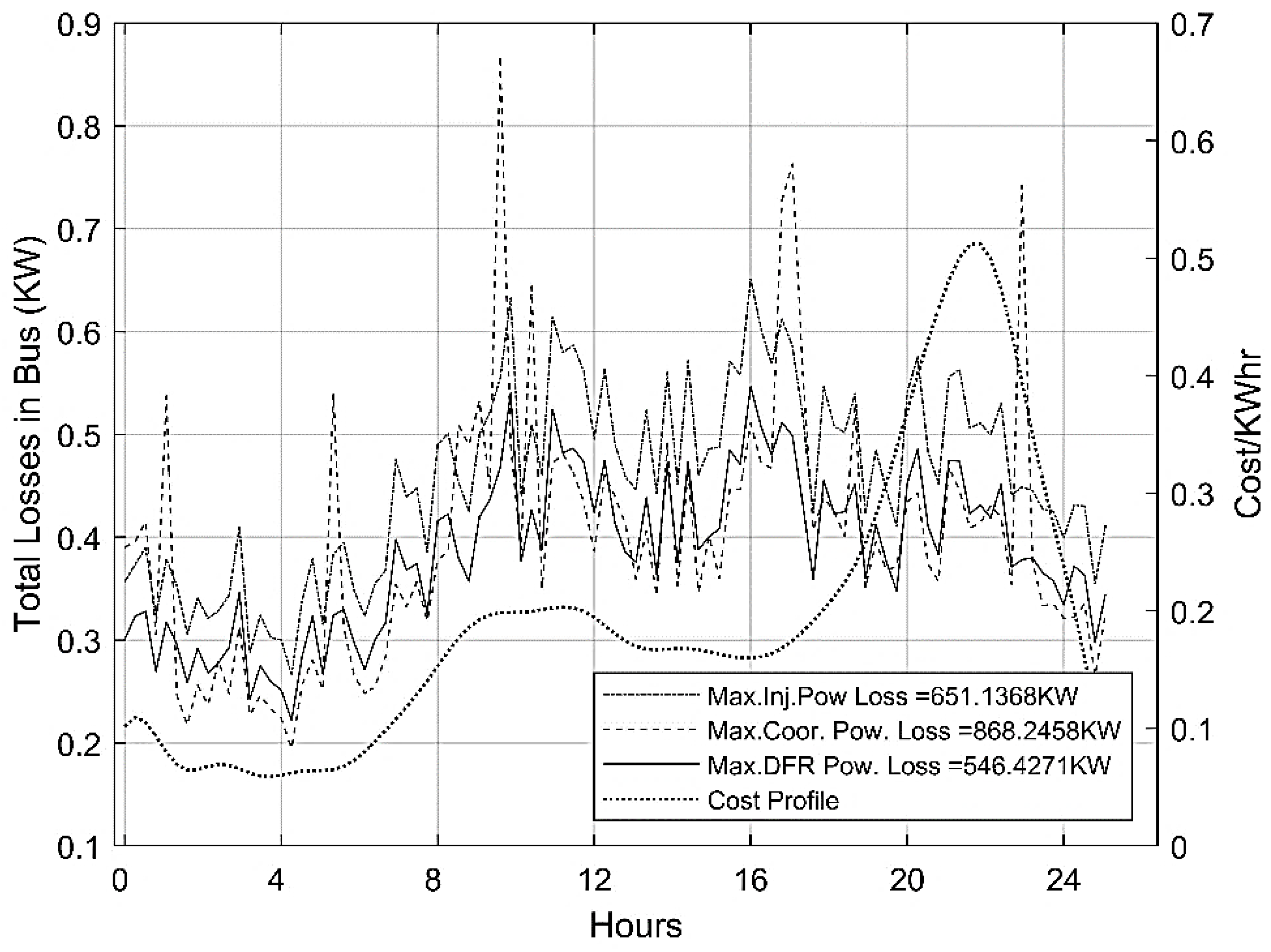
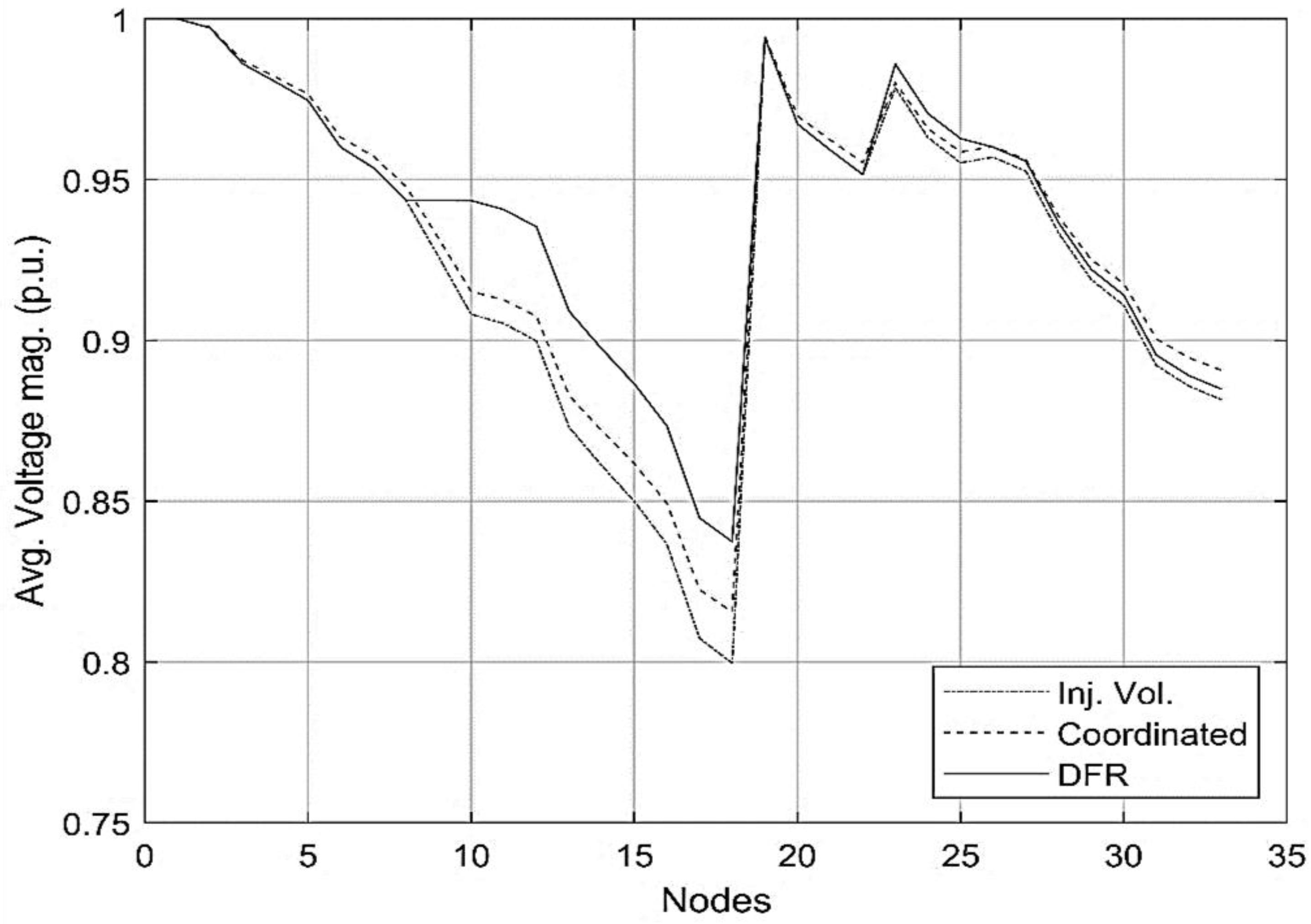
| No. | EV + Base Load Analysis | Optimization | Total Power Losses KW | Gen. Cost $ (1000) | Min. Voltage p.u. |
|---|---|---|---|---|---|
| 1 | Coordinated | MILP | 868 | 400 | 0.8 |
| 2 | Injection | Mixed Int. GA | 652 | 431 | 0.84 |
| 3 | DFR | MST *—GA | 546 | 429 | 0.87 |
Publisher’s Note: MDPI stays neutral with regard to jurisdictional claims in published maps and institutional affiliations. |
© 2022 by the authors. Licensee MDPI, Basel, Switzerland. This article is an open access article distributed under the terms and conditions of the Creative Commons Attribution (CC BY) license (https://creativecommons.org/licenses/by/4.0/).
Share and Cite
Nagi, F.; Azwin, A.; Boopalan, N.; Ramasamy, A.K.; Marsadek, M.; Ahmed, S.K. Comparison of Grid Reactive Voltage Regulation with Reconfiguration Network for Electric Vehicle Penetration. Electronics 2022, 11, 3221. https://doi.org/10.3390/electronics11193221
Nagi F, Azwin A, Boopalan N, Ramasamy AK, Marsadek M, Ahmed SK. Comparison of Grid Reactive Voltage Regulation with Reconfiguration Network for Electric Vehicle Penetration. Electronics. 2022; 11(19):3221. https://doi.org/10.3390/electronics11193221
Chicago/Turabian StyleNagi, Farrukh, Aidil Azwin, Navaamsini Boopalan, Agileswari K. Ramasamy, Marayati Marsadek, and Syed Khaleel Ahmed. 2022. "Comparison of Grid Reactive Voltage Regulation with Reconfiguration Network for Electric Vehicle Penetration" Electronics 11, no. 19: 3221. https://doi.org/10.3390/electronics11193221
APA StyleNagi, F., Azwin, A., Boopalan, N., Ramasamy, A. K., Marsadek, M., & Ahmed, S. K. (2022). Comparison of Grid Reactive Voltage Regulation with Reconfiguration Network for Electric Vehicle Penetration. Electronics, 11(19), 3221. https://doi.org/10.3390/electronics11193221