Article

Link-Aware Frame Selection for Efficient License Plate Recognition in Dynamic Edge Networks

1
School of Resources and Environment, University of Electronic Science and Technology of China, Chengdu 611731, China
2
School of Computer Science and Engineering, University of Electronic Science and Technology of China, Chengdu 611731, China
3
School of Information and Software Engineering, University of Electronic Science and Technology of China, Chengdu 611731, China
*
Author to whom correspondence should be addressed.
Electronics 2022, 11(19), 3186; https://doi.org/10.3390/electronics11193186
Submission received: 5 September 2022 / Revised: 18 September 2022 / Accepted: 27 September 2022 / Published: 4 October 2022
(This article belongs to the Special Issue Edge Computing for Urban Internet of Things)

Abstract

:
With the booming development of Internet of Things (IoT) and computer vision technology, running vision-based applications on IoT devices becomes an overwhelming tide. In vision-based applications, the Automatic License Plate Recognition (ALPR) is one of the fundamental services for smart-city applications such as traffic control, auto-drive and safety monitoring. However, existing works about ALPR usually assume that IoT devices have sufficient power to transmit the whole captured stream to edge servers via stable network links. Considering the limited resources of IoT devices and high-dynamic wireless links, this assumption is not suitable for realizing an efficient ALPR service on low-power IoT devices in real wireless edge networks. In this paper, we propose a link-aware frame selection scheme for ALPR service in dynamic edge networks aiming to reduce the transmission energy consumption of IoT devices. Specifically, we tend to select a few key frames instead of the whole stream and transmit them under good links. We propose a two-layer recognition frame selection algorithm to optimize the frame selection by exploiting both the video content variation and real-time link quality. The extensive results show that, by carefully selecting the offloaded frames to edge servers, our algorithm can significantly reduce the energy consumption of devices by 46.71 % and achieve 97.95 % recognition accuracy in the high-dynamic wireless link of the edge network.

1. Introduction

Recent years have witnessed the rapid development of the Internet-of-Things (IoT), a network connecting various devices over the Internet, where most connected devices can collect environmental data by embedded sensors and analyze the data by themselves [1,2]. In a smart city, operators usually deploy camera-equipped IoT devices in streets, crossroads and parks to collect relevant videos for complex computation applications, such as traffic controlling and smart parking [3]. ALPR [4] is an important service for smart traffic and controlling [5].
A significant feature in IoT is the cross-integration with existing technologies such as Computer Vision (CV), Natural Language Process (NLP), etc. With the rapid development and the popularity of IoT, there are more and more CV based applications being deployed on IoT devices in different scenarios such as face recognition in access control system, object detection in traffic system, etc. Currently, executing the CV-based services (such as ALPR) on low-power IoT devices is becoming a trending topic [6].
Traditional ALPR systems reply cloud servers for data processing. While cloud servers have sufficient computing power, they are too distant from IoT devices to provide a low-latency link and high quality services. In this context, edge computing [7] has emerged and is widely used. It is equivalent to deploying a small computing and data center close to the data source, which can temporarily store and analyze data, and then transmit them back to the cloud server as needed, greatly reducing the amount of transmitted data and relieving the pressure on the bandwidth of the central server. Compared to cloud-based ALPR, the edge-based ALPR has some unique features. (1) Much less round-trip time. The transmission process in edge computing is simplified from multi-hop backbone network communications to one-hop wireless communications, which can reduce the round-trip time from second level to millisecond level [8]. (2) One-hop wireless communication, which makes edge-based ALPR service more sensitive to the link variations than cloud-edge ALPR.
Most existing works about ALPR usually assume that IoT devices have sufficient power to transmit the whole captured streams to edge servers under stable network link. This assumption has two limitations. First, sending the whole stream to a remote server would consume considerable energy, which is unacceptable for low-power devices. Meanwhile, in most scenarios, a car will appear in multiple frames continuously [9] and thus it is not necessary to execute license plate recognition for all these frames. Second, wireless links in edge networks usually vary frequently and dramatically due to the interference of other signals and dynamic environments [10].
To address these problems, we propose a link-aware frame selection mechanism for automatic license plate recognition in dynamic edge networks, which particularly considers both the wireless network dynamics and the video content variation to select the appropriate frames offloaded to edge servers. Although such an idea is expected to significantly reduce the energy consumption of devices while guaranteeing the recognition accuracy.
  • The impact of dynamic wireless link on ALPR performance relies on the offloading results, while the frame selection needs to be determined before the offloading process.
  • Key frame selection. Wireless link dynamics and video content difference are two-dimension information, the set of recognition frames needs to be carefully selected with a joint consideration of these two variables.
To address these challenges, we propose a link-aware frame selection scheme with the following two innovations. First, we propose a novel and measurable metric, Normalized Key Frame Index (NKFI), to indicate the impact of wireless links on ALPR performance. With NKFI, the process of frame selection can be associated with real-time wireless link quality. Second, we design a two-layer recognition frame selection algorithm, which jointly considers both the wireless link quality and video content using the two metrics, Normalized Key Frame Index (NKFI) and Effective Frame Sampling Interval (EFSI).
The contributions of our work are summarized as follows.
  • We propose a link-aware frame selection scheme for Automatic license plate recognition service in dynamic edge networks. Distinct from most existing works, the proposed scheme suggests to offload a few key frames under the high-quality wireless links instead of the whole captured stream. In this way, the energy consumption for data transmission can be significantly reduced without losing much recognition accuracy for the ALPR service.
  • We devise two lightweight yet measurable metrics, Normalized Key Frame Index (NKFI) and Effective Frame Sampling Interval (EFSI), to indicate the process of frame selection. Based on these metrics, we design a two-layer recognition frame selection algorithm, which jointly considers the real-time link quality and video content variation.
  • We conduct extensive experiments to evaluate the performance of proposed scheme. The results show that, compared with existing works about ALPR, our scheme can significantly reduce the energy consumption of devices by 46.71 % and achieve 97.95 % recognition accuracy in the high-dynamic wireless link of edge network.
The rest of the paper is organized as follows. Section 2 discusses the related works. Section 3 describes the link-aware ALPR framework in edge computing. Section 4 presents the proposed two-layer recognition frame selection algorithm. Section 5 presents the evaluation results. Finally, Section 6 concludes the performance improvement of our work in this paper.

2. Related Work

In this section, we review the existing work and discuss their limitations. More specifically, Section 2.1 discusses the ALPR schemes from the perspective of computer vision. Section 2.2 summarizes the existing works about frame selection. Section 2.3 discusses the edge computing technology and justifies the position of our proposed method in edge computing.

2.1. Automatic License Plate Recognition

Existing ALPR systems can be mainly divided into two categories. The first category is based on traditional digital image processing (DIP) technology to optimize recognition accuracy. The second category is mostly end-to-end recognition framework systems based on deep learning. The traditional DIP-ALPR system usually includes four steps: Image Acquisition, License Plate Extraction [11], License Plate Segmentation [12] and Character Recognition. The performance of an ALPR system relies on the robustness of each individual step.
With the rise of Deep Learning (DL) techniques, the accuracy of many pattern recognition tasks was greatly improved. Target detection algorithms based on DL such as RCNN [13], Fast R-CNN [14], Faster R-CNN [15], SSD [16], and YOLO [17,18] series have emerged one after another. Consequently, the ALPR system based on DL grows rapidly. It simplifies the work into three steps: Vehicle Detection, License Plate Detection, and Optical Character Recognition (OCR) [19]. Many methods [20,21,22] achieve state-of-the-art performance in efficiency and accuracy.
However, DIP-ALPR and DL-ALPR either are based on image data or directly process video stream frame by frame. They often ignore the dynamic information between frames in the video such as “movement” information, which can be represented by the difference between frames. The small difference reflects slow “movement” and the large difference reflects fast “movement”. In this context, the second layer of our proposed two-layer scheme analyzes the “movement” information between frames by inter-frame difference. It achieves less overhead and offers adjustable parameters.
The work about ALPR can be further classified into two classes, one for cloud computing and the another one for edge computing. The existing works about cloud-based ALPR [23,24] usually aim at optimizing the recognition accuracy by complex yet efficient neural networks. For example, P. Kaur et al. [24] proposed a novel ALPR system based on a Convolutional Neural Networks (CNNs) for recognition, which can be used on a variety of vehicles and low-light conditions and achieve 98.13 % overall accuracy.
Existing works about edge-based ALPR [25,26], considering the limited resources of edge servers, usually focus on the design of lightweight ALPR models [25] and offloading strategies of ALPR streams [26]. For example, Tham, M. L. et al. [25] proposed a lightweight and accurate IoT-based ALPR solution using deep learning. However, its frames per second (FPS) is only 2.6 and license plate optical character recognition (OCR) accuracy is only 78.23 % . That means that the improvement of directly deploying deep learning models on IoT devices or improving them for IoT devices is limited, mainly due to the limited computing power of IoT devices. Therefore, our proposed method assigns high-load tasks to the edge server to complete, and the front-end IoT devices only need to select the tasks to be offloaded to the edge server through our proposed two-layer selection scheme. Yi, S. et al. [26] proposed a system built on top of an edge computing platform, which offloads computation between IoT devices and edge server. It achieves about 1.3–1.4 times faster response. Our proposed method puts more attention on saving energy of IoT devices and takes the varying link qualities into consideration. Our approach significantly reduces the energy cost while guaranteeing the recognition accuracy.

2.2. Key Frame Extraction Techniques

The key frame is the representative frame in the series of video frames. It can comprehensively reflect the main content of a video shot or even a whole video. As mentioned in Section 2.1, the first stage in ALPR is the license plate detection or extraction. The input for this stage is an image or a video. The output for this stage is then used for license plate location. This stage is very important as the result of the license plate recognition success rate is highly dependent on the image or the video frame. So for our edge-ALPR system, the quality of key frame extraction directly affects the recognition accuracy of the system.
Table 1 shows the categorizes, key ideas and limitations of the existing classic key frame extraction approaches. In summary, these existing efforts described above have limitations in terms of computational overhead or indication of changes. In contrast, our two-layer frame selection scheme advances in more complex scenarios.

2.3. Edge Computing

Edge computing, a distributed information technology (IT) architecture for computing on location where data are collected, enables IoT data to be gathered and processed at the edge instead of sending the data back to a data center or cloud. It occurs at or near the physical location of either the user or the data source.
One of the primary issues in edge computing is task offloading [31]. Task offloading is the process by which the edge server distributes a particular amount of computational resources to these uploaded apps in order to reduce latency or energy consumption and deliver a better user experience [32]. Typically, the decision about whether to offload is the first and most important step in computing offloads and resource allocations. Following the decision to offload, the next thing to address is how much and what should be offloaded. Our proposed method is in the position of the offload decision. On the one hand, in our proposed two-layer link-aware scheme, the first layer answers the question of how much should be offloaded at most, and the second link-aware layer answers which ones should be offloaded based on the video content and dynamic link quality. On the other hand, our proposed two-layer scheme can not only adapt to dynamic link changes in the one-hop “client-server” structure, but also save energy.

3. Edge-ALPR System Framework

We divide our work into three stages: video stream input, license plate detection and character recognition. The first stage is on IoT device. The second and third stage are on edge server.
  • Video Stream Input. We explore the “movement” information between frames by inter-frame difference. We propose two lightweight yet measurable metrics: Effective Frame Sampling Interval (EFSI) and Normalized Key Frame Index (NKFI) to determine how many frames we should select and which frames to be selected as key frames. We propose a new link-aware frame selection scheme to select the appropriate video frame. Then, we transmit the key frames to the edge server.
  • License Plate (LP) Detection. We first train and deploy the YOLOv3 [33] model, focusing on improving the vehicle detection speed. The network training dataset is a manually annotated dataset based on CCPD [34] (Chinese City Parking Dataset, ECCV). We then use RetinaFace [35] to perform transfer learning to realize license plate detection, four-corner positioning, license plate correction and alignment. Finally we extract the license plate area as the input to character recognition.
  • Character Recognition. We deploy an end-to-end convolutional neural network LPR-Net [36] without preliminary character segmentation. The network training dataset is a manually annotated dataset based on CCPD. We first perform image decolorization on the recognized color image of the license plate region. Then we input the processed grayscale image into the end-to-end deep learning network LPR-Net.
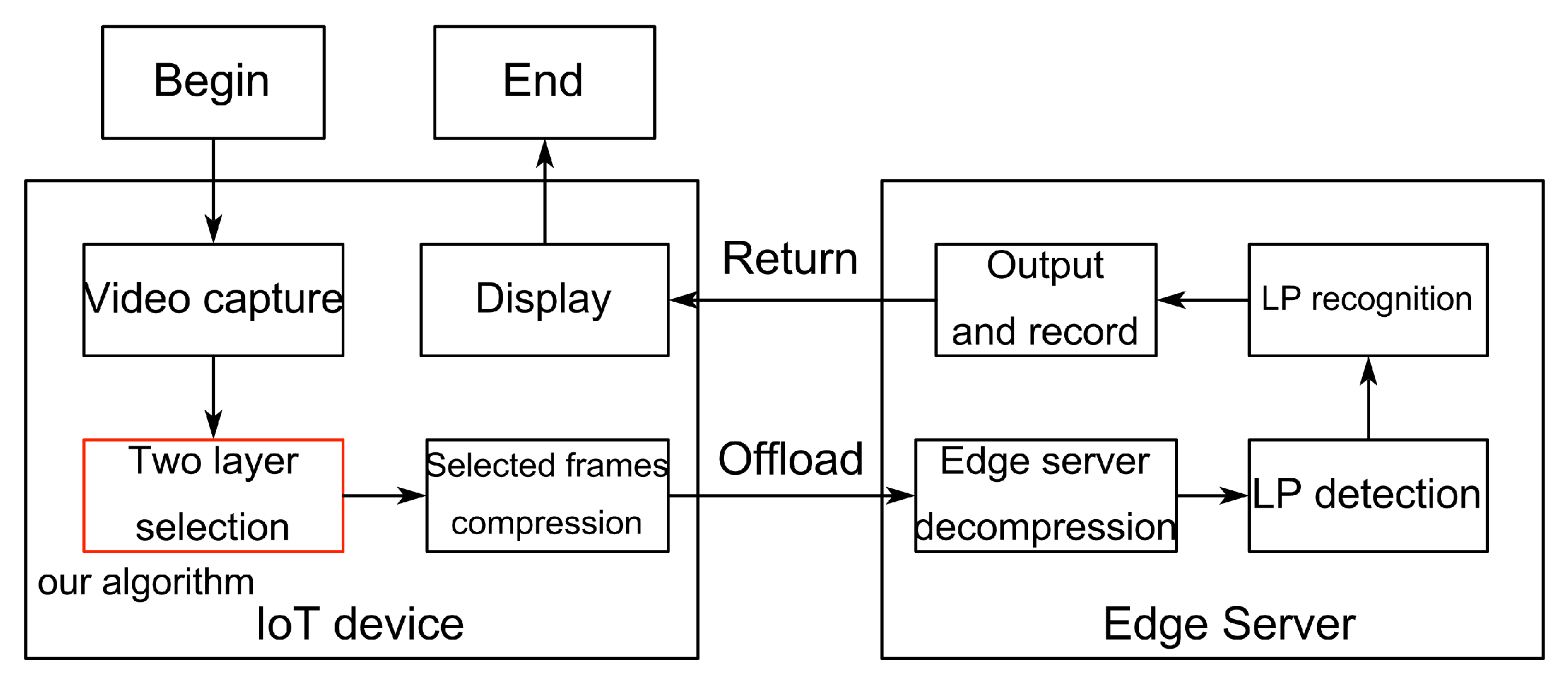
The entire framework of our edge-ALPR system is shown in Figure 1:

3.1. LP Detection

The vehicle is one of the basic objects in many classical detection and recognition datasets, such as ImageNet [37] and COCO dataset [38]. So we decide not to train the detector from scratch, but to utilize known models that meet our requirements. On the one hand, we expect a high recall rate as far as possible to accurately capture all the vehicle object in the scene. On the other hand, we hope to increase the detection speed and accuracy, while reducing the size of the model to facilitate deployment. Based on these considerations, we use two kinds of deep learning network YOLOv3 [33] and RetinaFace [35] for vehicle detection and license plate area detection. Instead of changing or optimizing the network structure, we just use the network as a black box, merging output related to vehicles and ignoring other categories. The network training dataset is a manually annotated dataset based on CCPD.
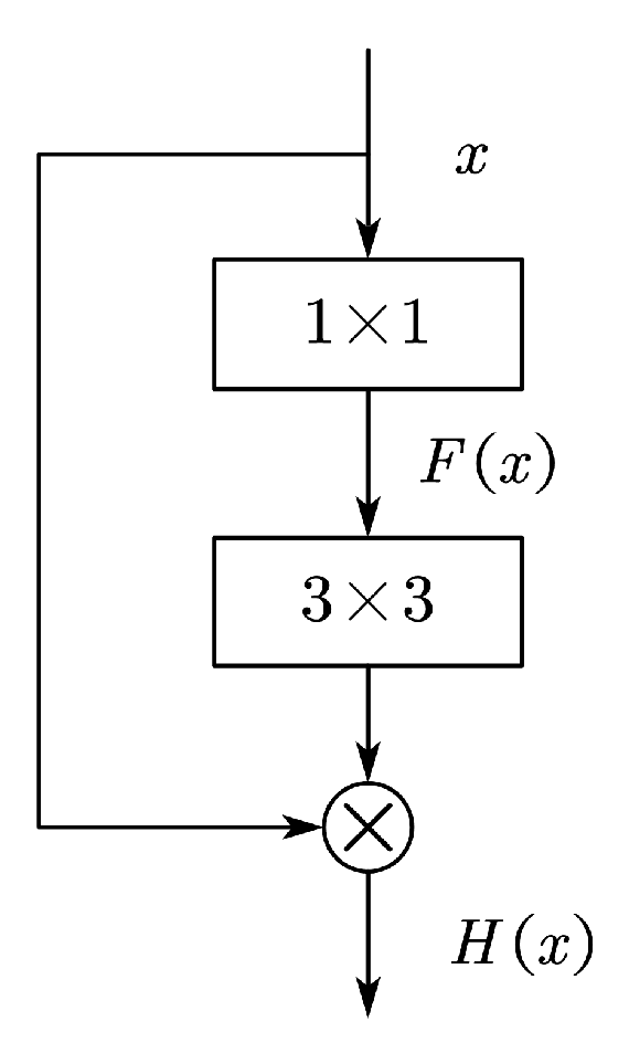
The YOLOv3 algorithm uses the network structure of DarkNet-53  [39] to extract the features of the vehicle information in the image, and uses the multi-scale detection method to detect the targets in the image. The image in the dataset is normalized to the size of 416 × 416 and sent into the network structure of the algorithm to detect the vehicle information. A large number of residual network structures with 1 × 1 and 3 × 3 convolution kernels are adopted in the DarkNet-53 network structure, referring to Figure 2.
The residual function of the residual network structure is:
F x = H x x
where F x represents the residual function of the residual network structure, H x represents the output value of the residual network structure, and x represents the input value of the residual network structure.
The input image of the network structure of the YOLOv3 algorithm is downsampled by a convolution layer with a step size of 2 for five times, and a total of five scales of characteristic images are obtained, which are 208 × 208 , 104 × 104 , 52 × 52 , 26 × 26 and 13 × 13 , respectively. The YOLOv3 algorithm inputs the feature graphs on the scales of 13 × 13 , 26 × 26 , 52 × 52 into the detection network for multi-scale detection. In the YOLOv3 algorithm, nine groups of anchor frames are evenly distributed on three scales of the detection network, and each anchor point of each scale is assigned three groups of anchor frames, resulting in a total of 10,647 anchor frames. YOLOv3 algorithm uses the Adam optimizer, which first uses regression to predict the category, confidence and prediction box of anchor frame, and then uses NMS algorithm to select the final prediction box according to the score of each prediction box. Finally, according to the relationship between the feature map and the original image, the prediction box is mapped to the original image to complete the location of the vehicle information in the image.
The formula for calculating confidence is:
C = P r object × I
P r object = 0 , no target 1 , target
where C indicates confidence; P r object indicates the probability that a target is detected in the prediction box; I represents the intersection ratio between the prediction box and the truth box area.
The formula for calculating the score of the target in the prediction box in the NMS algorithm is:
S = C × P r vehicle object
where S represents the score of the prediction box; P r logo object represents the conditional probability of the vehicle category.
RetinaFace [35] is a robust one-stage face detector with high speed and accuracy for small target recognition. When using MobilenetV1-0.25 as the backbone network, the model size is only 1.7 M, and it can achieve real-time detection. RetinaFace can also train other datasets on demand to achieve migration learning for other target recognition, so here we directly use a license plate correction and license plate detection model implemented using RetinaFace for migration learning.

3.2. Character Recognition

In this stage, we mainly use a combination of optical conventional image optimization methods and deep learning networks to recognize license plates. We first perform image decolorization on the recognized color image of the license plate region. Then we input the processed grayscale image into the end-to-end deep learning network LPR-Net [36], which finally achieves efficient and accurate license plate recognition and outputs the results.
Image decolorization refers to the conversion of color images to grayscale images, as Figure 3 shows. Image decolorization can simplify image information to save memory without affecting recognition accuracy. A color image has three components: red, green and blue. If red, green and blue are set to the same value, the image will become a gray image. The gray value is represented by a number between 0 and 255, which represents the gray depth between white and black. If there are only two gray values in an image, 0 and 255, we generally call it binarization.
Generally, the captured license plate images are acquired by digital camera shooting, so the images before pre-processing are color images. A color image, also known as an RGB image, uses three components R, G and B, to represent the color of a pixel. R, G and B represent red, green and blue, respectively, and any color can be synthesized by these three basic colors. Therefore, for a color image of size M × N , storing the image requires a three-dimensional array of M × N × 3 . The color image contains a large amount of color information, which not only has a high cost in storage but also slows down processing speed. Because each pixel of the image has three different color components of R, G and B, recognition does not use much of this information.
Therefore, before further processing, we convert the color image into a grayscale image to reduce memory cost. In the RGB model, if  R = G = B , the color represents a grayscale color, where the value of R = G = B is called the grayscale value. A grayscale image is an image that has only intensity information, but no color information. To store a grayscale image, only a two-dimensional matrix is needed, and each element of the matrix represents the grayscale value of the pixel at the corresponding position. The pixel color of a color image is R G B R , G , B , and the pixel color of a grayscale image is R G B r , r , r .
We use the weighted average method for image decolorization, referring to Formula (5)
r = R = G = B = R × W R + G × W G + B × W B 3
where W R , W G and W B are the weights of R, G and B respectively.
Studies [40] have shown that the human eye has the highest sensitivity to green, the second highest sensitivity to red, and the lowest sensitivity to blue. Therefore, we use the combination of weights ( W R = 0.299 , W G = 0.587 , W B = 0.114 ) that best matches the visual effect of the human eye to obtain the most reasonable grayscale image converted from the color image. Then we input the processed grayscale image into the end-to-end deep learning network LPR-Net.
LPR-Net [36] is an end-to-end Chinese license plate recognition method. LPR-Net is an efficient neural network with high recognition accuracy on challenging Chinese license plates dataset and can be trained end-to-end without considering specific details. LPR-Net is the first real-time license plate recognition system that does not employ RNNs [41]. It outperforms MSER-based and Color-based methods in terms of both recognition accuracy and robustness in complex environments. The structure of the backbone network is described in Table 2.
The backbone network acquires the images containing license plate as input and computes the spatial distribution of a large number of features. Wide convolution ( 1 × 13 convolution kernel) utilizes the local character context thus replacing the LSTM-based RNN network [41]. The output of the backbone sub-network can be considered as a sequence representing the possibility of the corresponding character, which has a length equal to the width of the input image. Since the output of the decoder is not aligned with the length of the target character sequence, the CTC Loss (Connectionist Temporal Classification Loss) function is employed for end-to-end training of the segmentation. CTC Loss function is a widely used method to deal with the misalignment of the input and output sequences.
LPR-Net consists of lightweight convolutional neural networks, so it can be trained using an end-to-end approach. It achieves an accuracy of 95 % for Chinese license plate recognition.

4. Design

4.1. Overview

Image a scene where an ordinary camera used for road monitoring has 30 m to 60 m HD-shooting-distance and 30 frame rate. When a car with a speed of 60 km/h passes the camera, it takes about 2 s to pass through the camera’s HD-shooting-area, and the camera has already captured about 60 frames for the same object. Given a sequence of frames F = f i , , f i + n 1 , then obviously the subset F j = f j , , f j + 59 where j = i , i + 1 , , i + n 60 may contain the same object for all frames, which means we detect one object 60 times at most when we do object detection frame by frame. It is heavy and redundant for low-power IoT devices.
To reduce the workload on the edge as much as possible, the selected key frames should capture as much movement as possible, and not have much redundancy between each other. So there are two key problems:
1. How many frames to select?
2. Which frames to select?
Meanwhile, another problem is that wireless links in edge networks usually vary frequently and dramatically due to the interference of other signals and dynamic environments.
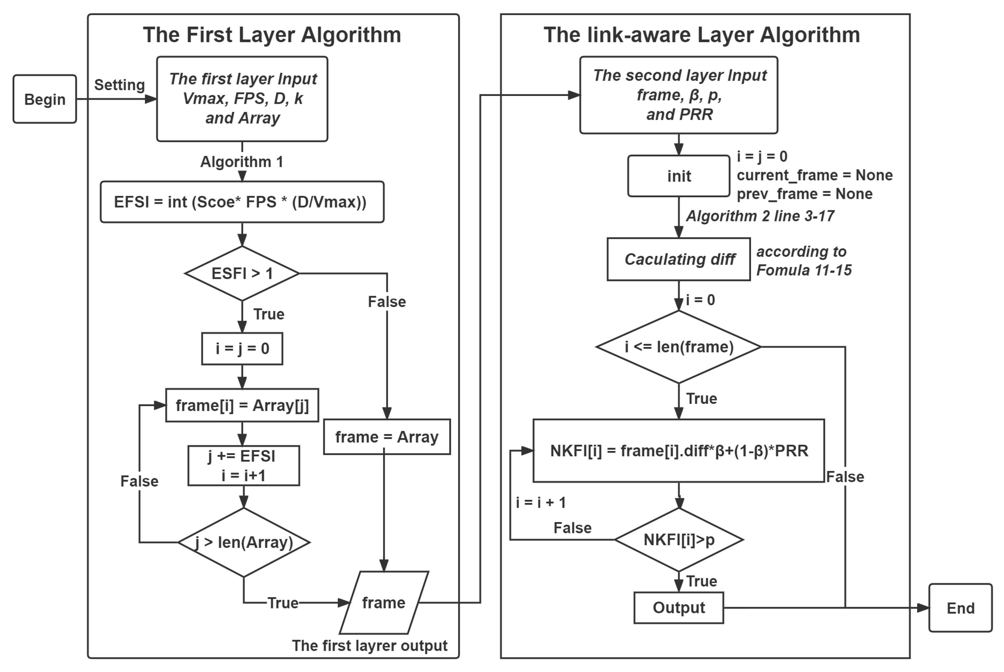
To address these problems, we propose a two-layer link-aware frame selection scheme, which particularly considers both the wireless network dynamics and the video content variation to select the appropriate frames offloaded to edge servers. It is mainly consist of two core metrics: Effective Frame Sampling Interval (EFSI) and Normalized Key Frame Index (NKFI). Algorithm 1 shows the process of the first layer selection. Algorithm 2 shows the process of the link-aware layer selection. Figure 4 shows the flowchart of our proposed two-layer algorithm.
Algorithm 1 The First Layer Algorithm of our Scheme
Input: 
V m a x : Max speed of car (km/h); F P S : Frame number per second of video;
D: Camera HD-shooting distance; k : The ratio of detection failure each frame;
A r r a y : video stream data;
Output: 
f r a m e : The first layer selection result.
1:
V m a x V m a x / 3.6
2:
S c o e 1 / l o g 1 k 1000
3:
m a x _ s a m p l i n g _ i n t e r v a l F P S · D V m a x
4:
E S F I S c o e · m a x _ s a m p l i n g _ i n t e r v a l
5:
i 0
6:
while i l e n ( A r r a y ) do
7:
   f r a m e A r r a y [ i ]
8:
   i i + E F S I
9:
end while
10:
return f r a m e
Algorithm 2 The Link-aware Layer Algorithm of our Scheme
Input: 
f r a m e : The first layer selection result.
β : Weight value; p: Threshold for N K F I i ;
P R R : Packet Reception Ratio;
Output: 
K F S : Key-frame-sequence.
1:
c u r r _ f r a m e , p r e v _ f r a m e N o n e
2:
i , j 0
3:
while i l e n ( f r a m e ) do
4:
   c u r r _ f r a m e f r a m e [ i ]
5:
   i + +
6:
  if c u r r _ f r a m e and p r e v _ f r a m e then
7:
    d i f f c u r r _ f r a m e p r e v _ f r a m e
8:
    C a l c u l a t e T 0 , μ 1 , μ 2 , a 1 , a 2 , T h     ▹ According to Fomulas (11)–(13)
9:
    d i f f T h r e s h o l d ( d i f f , T h , 255 )          ▹ Binarization
10:
    k e r n e l G e t S t r u c t u r i n g E l e m e n t ( c v 2 . M O R P H _ R E C T , ( 7 , 7 ) )
11:
    d i f f E r o d e ( d i f f , k e r n e l )              ▹ Erode
12:
    d i f f D i l a t e ( d i f f , k e r n e l )              ▹ Dilate
13:
    f r a m e s . a p p e n d ( F r a m e ( j , ( d i f f ) )
14:
    j + +
15:
  end if
16:
   p r e v _ f r a m e c u r r _ f r a m e
17:
end while
18:
f r a m e s . s o r t ( k e y d i f f , r e v e r s e T r u e )      ▹ sort in descending order
19:
m a x _ d i f f f r a m e s [ 0 ] . d i f f
20:
i 0
21:
for i 0 r a n g e ( l e n ( f r a m e s [ : ] ) ) do
22:
   f r a m e s [ i ] . d i f f f r a m e s [ i ] . d i f f / m a x _ d i f f
23:
   N K F I [ i ] f r a m e s [ i ] . d i f f · β + ( 1 β ) · P R R
24:
  if N K F I [ i ] > p then
25:
    K F S . a p p e n d ( f r a m e s [ i ] )
26:
  end if
27:
end for
28:
return K F S

4.2. Metrics and Algorithm Statement

Effective Frame Sampling Interval (EFSI). We find that in most cases we only need a few frames to accurately identify the same one object. So we define the Effective Frame Sampling Interval (EFSI) metric as follows:
E F S I = S c o e · F P S · D V m a x
m a x _ s a m p l i n g _ i n t e r v a l = F P S · D V m a x
where S c o e indicates sampling coefficient between 0 to 1; F P S indicates the number of frames per second; D indicates the minimum of the camera’s HD-shooting-distance; V m a x represents the max speed allowed on the road and needs to be transferred from km/h to m/s; We sort out some common application scenarios and corresponding parameters as Table 3:
We call F P S · D V m a x the m a x _ s a m p l i n g _ i n t e r v a l , because it represents the minimum number of frames of the same object target in the video frame sequence. For instance, for a car with 120 km/h speed on highway, 24 F P S , D of the camera is 30 m, then m a x _ s a m p l i n g _ i n t e r v a l is 21, which means this car shows up 21 times in the video frame sequence. Moreover, if we let EFSI equal to m a x _ s a m p l i n g _ i n t e r v a l , the frame-sampling-sequence will have only one frame containing this car.
However, letting EFSI simply equal to m a x _ s a m p l i n g _ i n t e r v a l is risky, because that there is a chance the object cannot be detected in the only frame due to occlusion. So, we define the sampling coefficient S c o e , referring to the Formula (8):
S c o e = 1 log 1 k 1000
where k is an independent constant between 0 to 1 indicating the probability of detection failure of each frame. Based on our experiments, k = 1 / 10 can satisfy the scenarios we list. S c o e guarantees the overall ratio of detection failure in all selected frames containing the same one object could be less than 1 / 1000 .
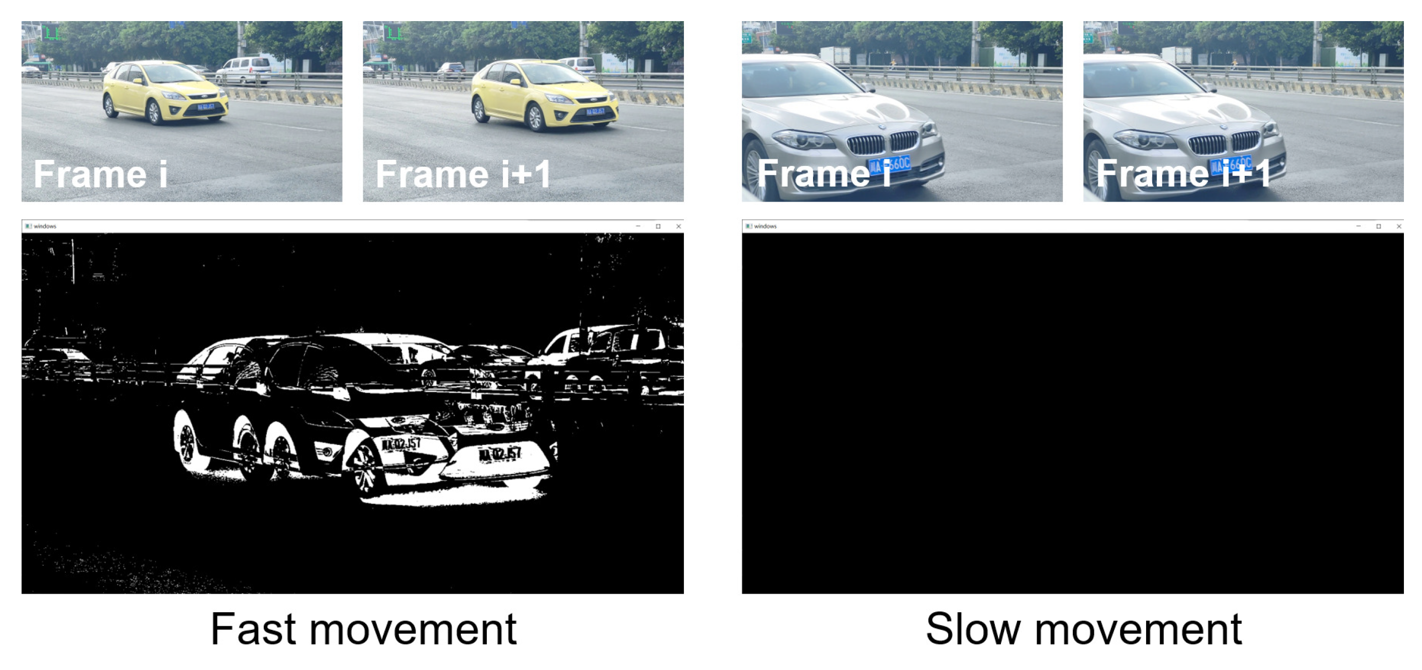
Normalized Key Frame Index (NKFI). According the Formula (6), we get the frame-sampling-sequence. We use a lightweight i n t e r - f r a m e d i f f e r e n c e function to calculate the “movement” between two frames (Figure 5 and Figure 6). We define Normalized Key Frame Index (NKFI) as the weighted average of the inter-frame difference and the wireless link quality metric packet reception rate ( P R R ).
First, we convert the frame to grayscale and compute the absolute difference of pixel values d i , j ( x , y ) for every pixel (x,y) between frame i and frame j, and consider it significant if it exceeds a threshold Th:
d i , j x , y = f i x , y f j x , y
t i , j x , y = 1 , d i , j x , y > Th 0 , otherwise
However, if the threshold Th is too high, the moving target region will be seriously fragmented. and if the threshold Th is too low, a lot of noise will be introduced. Therefore, we use a dynamic threshold by calculating the gray value of the current image:
(a) Obtain the minimum and maximum gray values in the image, and take the average value as the initial threshold T 0 .
(b) Divide the image into the target part and the background part by threshold T 0 . Obtain the average gray values μ 1 and μ 2 and the gray probability a 1 and a 2 of two parts.
μ 1 = f i , j x , y < T 0 f i , j x , y f i , j x , y < T 0 N , μ 2 = f i , j x , y T 0 f i , j x , y f i , j x , y T 0 N
a 1 = f i , j x , y < T 0 f i , j x , y f i , j x , y , a 2 = f i , j x , y T 0 f i , j x , y f i , j x , y
(c) Dynamic threshold Th can be calculated as:
Th = a 1 · a 2 · μ 1 + μ 2
We then use morphological operations such as erode and dilate to eliminate the white noise caused by camera jitter and wind blowing leaves. We compute the frame difference t i , j between frame i and frame j and normalize it as:
t i , j = x , y t i , j x , y , t i , j 0
t i , j = t i , j max i , j t i , j
We take P R R [42] (Packet Reception Ratio) as the indicator to reflect the current link quality. It is computed as the ratio of the number of successfully received packets to the number of transmitted packets. Setting β 0 < β < 1 , we define NKFI and append the frame that NKFI i > p (base on our experiment, we pick p = 0.35 ) into the final key frame sequence.
NKFI i = β · t i , i + 1 + 1 β · P R R
where P R R indicates the wireless link quality, between 0 to 1: the higher, the more stable.

5. Evaluation

Based on a series of simulations, this section sets up five independent cases and compares the performance with each other to analyze the effectiveness and efficiency of our proposal in different application scenarios.

5.1. Evaluation Setup

The workflow of edge-based ALPR system is shown as Figure 7. Our proposed algorithm runs on the IoT device to select the frames that meet the constraints of our two-layer scheme. The detection part by deep learning runs on the edge server to detect the license plate area and recognize it. The IoT device first captures video through a camera and runs our proposed two-layer algorithm to select frames that satisfy the conditions, which are then compressed and offloaded to the nearest edge server by wireless network. The edge server obtains and decompresses the image sequence for vehicle detection, license plate detection and license plate recognition, and outputs the results. Finally, the edge server returns recognition results back to IoT devices to display.
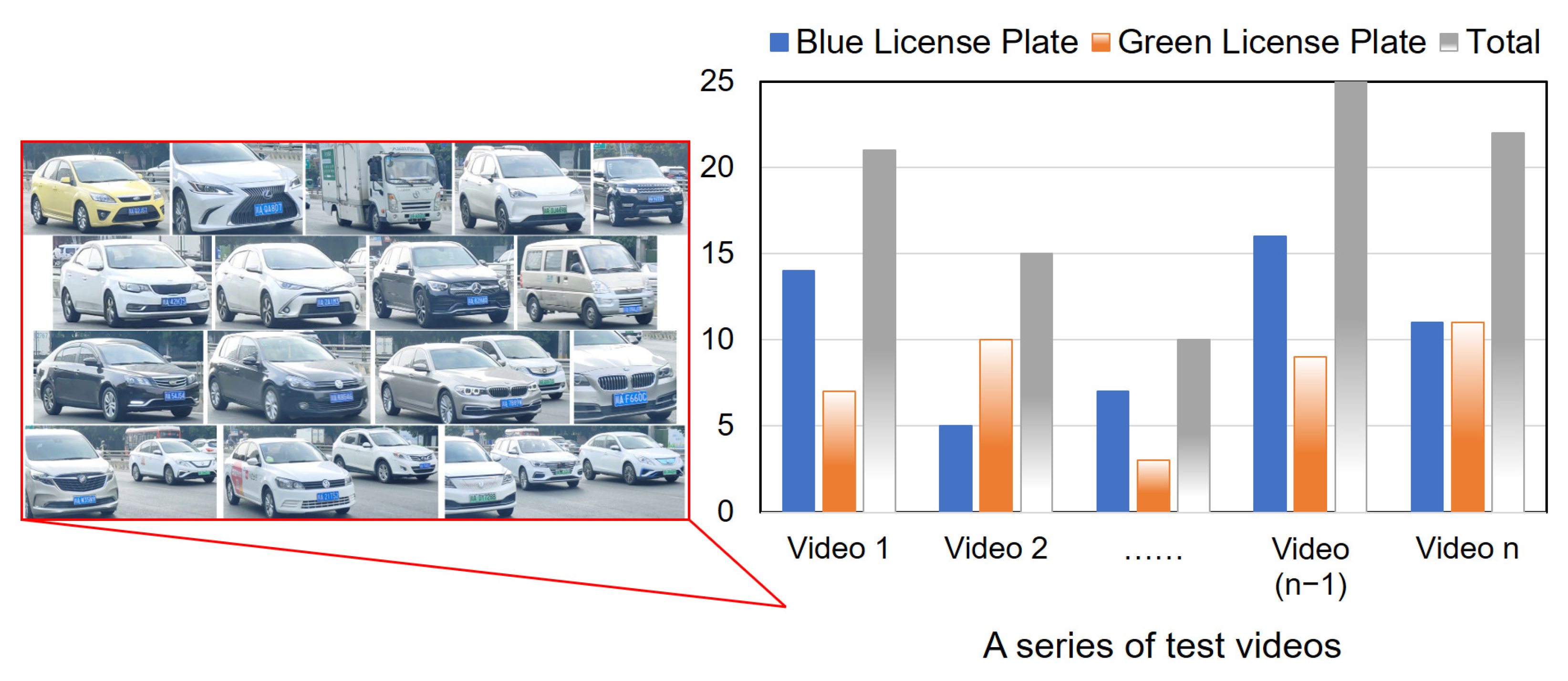
The operating system of the simulation experiment is Ubuntu18.04.6 LTS, and used package are CUDA11.6, Pytorch1.12.1, OpenCV4.6.0. We use an android phone with a 13 million pixel camera as the IoT device, and a laptop with a NVIDIA GTX1650 as the edge server. Considering that in most practical situations, the camera has a certain height and angle from the ground, which naturally avoids some miscapture. So we use a tilt of 45 degrees to capture video stream data to avoid overlap as much as possible. The test data are a series of 20-s videos by mobile phone, 1080p, 30 FPS, with 600 frames of each video. For instance, as Figure 8 shows, video 1 has, in total, 21 cars passing through, including 14 blue license plates and 7 green license plates.
Our proposed algorithm has two features: On the one hand, it adds the selection of sampling and the “movement” information between frames; On the other hand, it utilizes both information of link quality and inter-frame difference to determine key frames. Therefore, we specifically analyze the effect of these two features on the performance improvement separately.
We set up five independent cases to test and analyze the performance improvement of our scheme. The A c c u r a c y ( / % ) is defined as the number of recognition success frames divided by the number of frames with full license plate number. The E x t r a c t i o n _ q u a l i t y ( / % ) is defined as the number of frames with full license plate number divided by total number of frames. The E n e r g y _ l o s s ( / % ) is defined as average energy overhead divided by the overhead of CASE 1. The average energy overhead is represented by the average energy consumption in the process of transmitting key frames to the edge server.
  • Frame by frame, no frame selection;
  • Only the first layer selection (i.e., equally spaced sampling);
  • Only the link-aware layer selection (i.e., inter-frame difference frame by frame);
  • Two-layer selection, but β = 0 (link-unaware);
  • Two-layer selection, and β = P R R (link-aware);
CASE 1: IoT device sends video data to server without frame selection.
CASE 2: Set parameters according to mobile phone configuration and actual conditions. For instance, one group parameter for urban road could be: V m a x = 60 km/h = 16.6 m/s, F P S = 30 , D = 10 m, k = 1 / 10 . It means when a car passes camera shooting area (10 m) with max speed (60 km/h) allowed, we record it for at least 18 frames in video sequence and extract 1 frame as key frame every 6 continuous frames in video sequence. We sample and extract at least 3 frames containing one same car for the next detection and recognition.
CASE 3: Calculate the “movement” information frame by frame in whole video and output the key frame sequence.
CASE 4: Set the same parameters as CASE 2. We first use the first layer to sample frames that are effective enough to be detected. We then calculate its significance by metric NKFI (but β = 0 ). In this case, it is a link-unaware frame selection scheme.
CASE 5: Set the same parameters as CASE 2 and β = P R R . In this case, it is our link-aware frame selection scheme. Final output is the key frame sequence according to Algorithm 2.

5.2. Performance Improvement Analysis

5.2.1. Comparison of A c c u r a c y and E x t r a c t i o n _ q u a l i t y

Figure 9 shows the comparison of CASE 1, CASE 2 and CASE 5. The performance of A c c u r a c y and E x t r a c t i o n _ q u a l i t y in each video is considered as independent and only influenced by its own scenario and environment conditions. Among them, video 1 has regular density of traffic on urban road and good weather condition; Videos 2–4 has sparse density of traffic on urban road and good weather condition; Video 5 have sparse density of traffic on urban road and poor weather condition. Video 6 has crowded traffic and raining weather condition on urban road, which is the most complex scenario in our experiment. Videos 7–10 contain different scenarios such as street, school, hospital and parking lot, rather than the urban roads in videos 1–6.
For each video, we simulate 20 times to take average result to compare and analyze, as shown in Table 4.
Figure 9a shows the A c c u r a c y of CASE 1, CASE 2 and CASE 5 in different scenarios. Figure 9b shows the E x t r a c t i o n _ q u a l i t y of CASE 1, CASE 2 and CASE 5 in different scenarios. As shown in Figure 9a, CASE 5’s accuracy is consistently higher than CASE 1 and CASE 2. This is mainly because the ratio of frames that can not be successfully recognized decreases by culling frames with low N K F I , which mainly are foreground-occluded frames, overlapping frames, etc. CASE 1’s accuracy is 94.93 % on average and up to 95.12 % . CASE 2’s accuracy is 96.21 % on average and up to 96.31 % . CASE 5’s accuracy is 97.95 % on average and up to 98.31 % . The accuracy improvement of the CASE 5 algorithm over CASE 1 is 3.18 % on average and up to 3.45 % . The accuracy improvement of the CASE 5 algorithm over CASE 2 is 1.81 % on average and up to 2.00 % . Especially in video 6, which has crowded traffic and bad weather condition, CASE 1 has the worst behavior. However, CASE 5 extracts all cars out and avoids the influence of dim weather light, achieving 97.65 % accuracy. As shown in Figure 9b, CASE 5’s extraction quality is also consistently higher than CASE 1 and CASE 2. In addition, CASE 5 achieves better stability than CASE 1 and CASE 2, which is 83.37 % on average an up to 84.40 % . CASE 2 has the worst behavior about extraction quality, which is 58.84 % on average and low to 56.29 % . It means that CASE 2 picks up much more frames (close to 1.69 times) than the minimum workload we wish. It is mainly because it doesn’t have adaptive ability with traffic flow. For instance, when the traffic flow is sparse or even there are no vehicles for a period of time, it is also sampling at equal intervals, causing unnecessary waste. CASE 1’s (frame by frame) “extraction” quality is 73.34 % on average and up to 77.2 % . The extraction quality improvement of CASE 5 algorithm over CASE 1 reaches an average of 13.68 % and 21.15 % at most. The extraction quality improvement of CASE 5 algorithm over CASE 2 reaches an average of 41.69 % and 48.49 % at most.
We can conclude that: (1) From the difference between CASE 5 and CASE 2, our practice of setting the link-aware layer can improve the accuracy performance by about 1.81 % to 2.00 % , achieving 97.95 % accuracy on average and 98.31 % at most. (2) From the difference between CASE 5 and CASE 2, our practice of setting the link-aware layer can improve the extraction quality performance by about 41.69 % on average and 48.49 % at most. (3) From the difference between CASE 1 and CASE 2, our practice of setting the first layer can improve the accuracy performance by about 1.3 % on average, but degrades extraction quality performance by about 19.77 % on average due to poor adaptive ability with traffic flow.
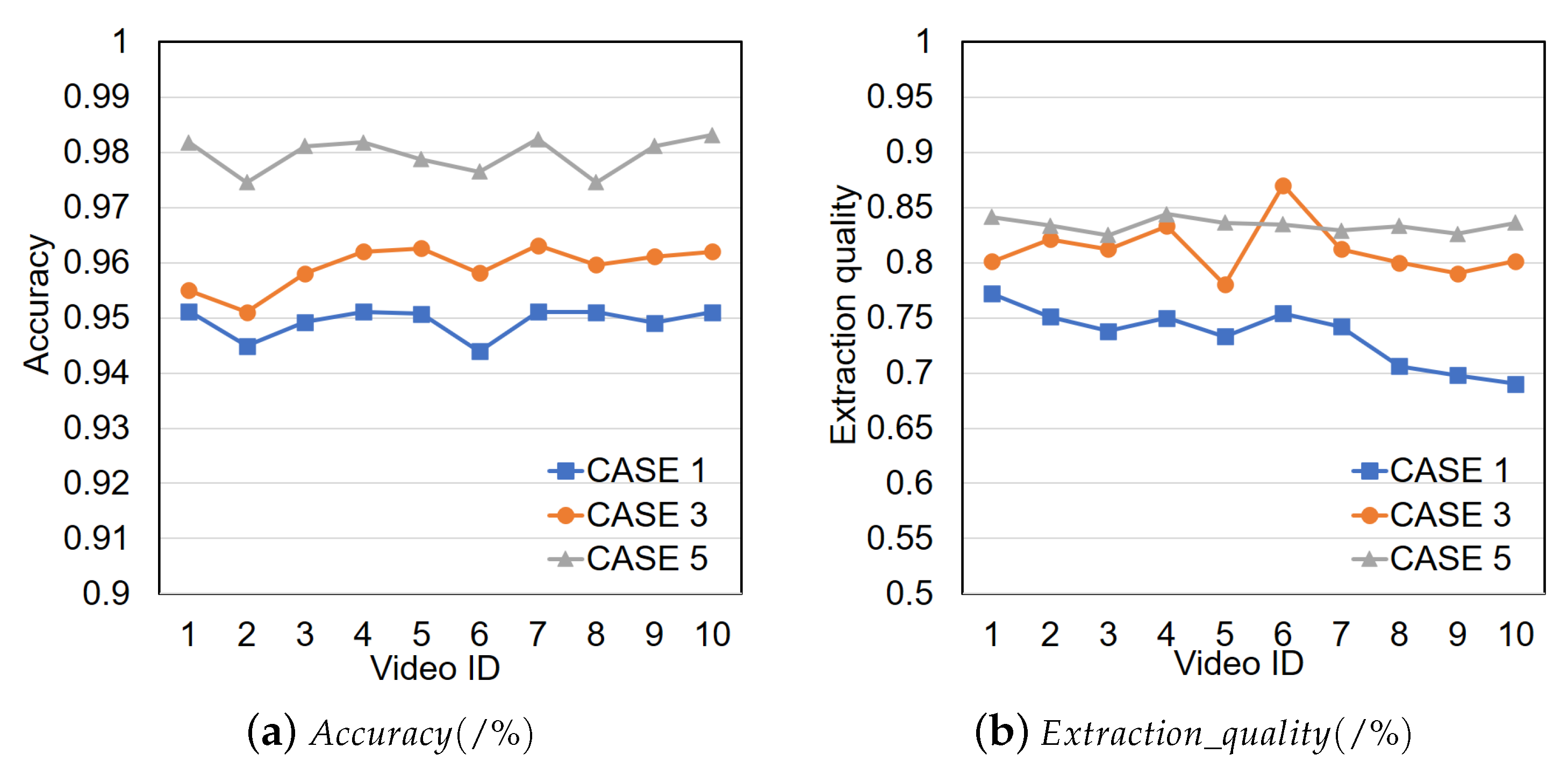
Figure 10 shows the comparison of CASE 1, CASE 3 and CASE 5. Figure 10a shows the A c c u r a c y of CASE 1, CASE 3 and CASE 5 in different scenarios. Figure 10b shows the E x t r a c t i o n _ q u a l i t y of CASE 1, CASE 3 and CASE 5 in different scenarios. As shown in Figure 10a, CASE 5’s accuracy is consistently higher than CASE 1 and CASE 3. CASE 3’s accuracy is 95.92 % on average and up to 96.33 % . The accuracy improvement of CASE 5 over CASE 3 is 2.11 % on average and up to 2.81 % . As shown in Figure 10b, CASE 5’s extraction quality is mostly higher than CASE 3, except video 6, due to its crowded traffic. The key idea of CASE 3 is calculating the “movement” information frame by frame in whole video by inter-frame difference but not sampling first. This helps CASE 3 capture more “movement” information and discard the “static” frame as much as possible. So it let CASE 3 keep more frame number of full detection with license plate in total number and get higher extraction quality in scenario with crowded traffic. In addition, for videos 2–4 and video 7 which have sparse density of traffic, CASE 5’s extraction quality is close to CASE 3. Similarly, it is mainly caused by the sparse traffic in videos 2–4 and video 7. Though CASE 3 has better behavior than CASE 5 in some specific scenarios about extraction quality, CASE 3’s “extraction” quality is 81.20 % on average and up to 87.01 % . The extraction quality improvement of CASE 5 algorithm over CASE 3 reaches an average of 2.67 % and 7.16 % at most. The extraction quality improvement of CASE 3 algorithm over CASE 1 reaches an average of 10.72 % and 16.11 % at most.
We can conclude that: (1) From the difference between CASE 5 and CASE 3, our practice of setting the first layer can improve the accuracy performance by about 2.11% to 2.81%, achieving 97.95 % accuracy on average and 98.31 % at most. (2) From the difference between CASE 5 and CASE 3, our practice of setting the first layer can smooth the extraction quality performance. Just for extraction quality, CASE 3 may have better behaviors in some scenarios with crowded traffic. (3) From the difference between CASE 3 and CASE 1, setting the link-aware layer improves the extraction quality performance by about 10.72 % on average and 16.11 % at most.
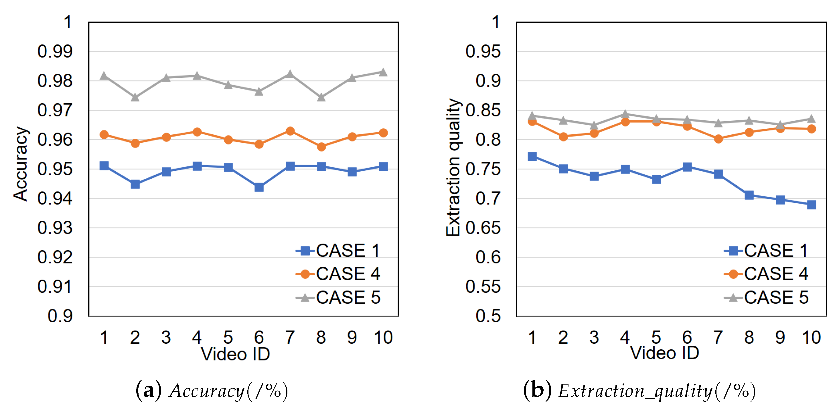
Figure 11 shows the comparison of CASE 1, CASE 4 and CASE 5. Figure 11a shows the A c c u r a c y of CASE 1, CASE 4 and CASE 5 in different scenarios. Figure 11b shows the E x t r a c t i o n _ q u a l i t y of CASE 1, CASE 4 and CASE 5 in different scenarios. As shown in Figure 11a, CASE 5’s accuracy is consistently higher than CASE 1 and CASE 4. CASE 4’s accuracy is 96.07 % on average and up to 96.31 % . The accuracy improvement of the CASE 5 algorithm over CASE 4 is 1.95 % on average and up to 2.14 % . Both of CASE 4 and CASE 5 have stable accuracy performance over 96 % in our experiments. As shown in Figure 11b, CASE 5’s extraction quality is mostly higher than CASE 4. CASE 4’s “extraction” quality is 81.87 % on average and up to 83.11 % . The extraction quality improvement of CASE 5 algorithm over CASE 1 reaches an average of 13.68 % and 21.15 % at most. The extraction quality improvement of CASE 5 algorithm over CASE 4 reaches an average of 1.83 % and 3.45 % at most. The extraction quality improvement of CASE 4 algorithm over CASE 1 reaches an average of 11.63 % and 18.63 % at most. CASE 4’s extraction quality is closer to CASE 5 and smoother than CASE 3. It is mainly caused by the metric EFSI as mentioned before. CASE 4 mainly uses both EFSI and NKFI metrics to extract key frame, but β = 0 .
We can conclude that: (1) From the difference between CASE 5 and CASE 4, considering the link quality influence can improve the accuracy performance by about 1.95 % to 2.14 % , achieving 97.95 % on average and 98.31 % at most. (2) For extraction quality performance, considering link quality influences it slightly on average.

5.2.2. Comparison of E n e r g y _ l o s s

Figure 12 compares the E n e r g y _ l o s s ( % ) of the five cases: CASE 1, CASE 2, CASE 5, CASE 3 and CASE 4. The E n e r g y _ l o s s ( % ) is defined as test average overload divided by CASE 1 overload. The E n e r g y _ l o s s ratio is a normalized performance metric that reflects overhead (i.e., the sum of energy usage of IoT device) compared with CASE 1 for the same task. As shown in Figure 12 (Displayed in logarithmic form), CASE 2’s E n e r g y _ l o s s is lowest of the five cases and CASE 3 consumes the most energy. CASE 2’s average E n e r g y _ l o s s is 30.61 % . CASE 5’s average E n e r g y _ l o s s is 53.29 % . CASE 3’s average E n e r g y _ l o s s is 293.75 % . CASE 4’s average E n e r g y _ l o s s is 52.63 % . The E n e r g y _ l o s s improvement of the CASE 2 over CASE 1 is 69.39 % . According to Figure 9b, though CASE 2 has the lowest overhead, it has the worst extraction quality. The E n e r g y _ l o s s improvement of the CASE 5 over CASE 1 is 46.71 % , and CASE 5 has the best behavior of accuracy and extraction quality. The E n e r g y _ l o s s improvement of the CASE 3 over CASE 1 is 193.75 % , which means CASE 3’s overhead is almost three times CASE 1’s. Although CASE 3 has great behavior of accuracy and extraction quality, the corresponding cost is too high. The E n e r g y _ l o s s improvement of the CASE 4 over CASE 1 is 47.37 % , close to CASE 5’s behavior. It’s mainly because the only difference between CASE 5 and CASE 4 is β , making little impact on the time complexity of the algorithm.
We can conclude that: CASE 5 shows great performance in E n e r g y _ l o s s , which saves 46.71 % energy compared with CASE 1. In addition, based on comparison of A c c u r a c y and E x t r a c t i o n _ q u a l i t y , CASE 5 consistently outperforms CASE 1, CASE 2, CASE 3 and CASE 4. Thus, CASE 5 is a good method to extract key frame sequence of video stream in edge ALPR system based on low-power IoT device.

6. Conclusions

In this paper, we propose a two-layer link-aware frame selection scheme for ALPR service in the dynamic wireless links of edge networks. The distinctive feature of our scheme is that we exploit both the video content variation and real-time link quality. We set up five independent experiment cases and analyze the performance improvement of each layer of our scheme. The extensive experimental results show that our scheme exhibits superior performance of A c c u r a c y , E x t r a c t i o n _ q u a l i t y and E n e r g y _ l o s s in different scenarios. Compared with no frame selection, our scheme can significantly reduce the energy consumption of devices by 46.71% and achieve 97.95% recognition accuracy in the high-dynamic wireless link of edge network.

Author Contributions

Methodology, J.L.; Resources, Y.Z.; Validation, J.L. and X.W.; Writing—original draft, J.L. and Y.Z.; Writing—review & editing, R.C. and X.W. All authors have read and agreed to the published version of the manuscript.

Funding

This work was supported by the National Natural Science Foundation of China (No. 61972074) and the National Key Research and Development Program of China (No. 2020YFE0200500).

Data Availability Statement

Not applicable.

Conflicts of Interest

The authors declare no conflict of interest.

References

  1. Guo, F.; Yu, F.R.; Zhang, H.; Li, X.; Ji, H.; Leung, V.C. Enabling massive IoT toward 6G: A comprehensive survey. IEEE Internet Things J. 2021, 8, 11891–11915. [Google Scholar] [CrossRef]
  2. Shu, C.; Zhao, Z.; Min, G.; Hu, J.; Zhang, J. Deploying network functions for multiaccess edge-IoT with deep reinforcement learning. IEEE Internet Things J. 2020, 7, 9507–9516. [Google Scholar] [CrossRef]
  3. Agarwal, Y.; Ratnani, P.; Shah, U.; Jain, P. IoT based smart parking system. In Proceedings of the 2021 5th International Conference on Intelligent Computing and Control Systems (ICICCS), Madurai, India, 6–8 May 2021; pp. 464–470. [Google Scholar]
  4. Du, S.; Ibrahim, M.; Shehata, M.; Badawy, W. Automatic license plate recognition (ALPR): A state-of-the-art review. IEEE Trans. Circuits Syst. Video Technol. 2012, 23, 311–325. [Google Scholar] [CrossRef]
  5. Khan, L.U.; Yaqoob, I.; Tran, N.H.; Kazmi, S.A.; Dang, T.N.; Hong, C.S. Edge-computing-enabled smart cities: A comprehensive survey. IEEE Internet Things J. 2020, 7, 10200–10232. [Google Scholar] [CrossRef] [Green Version]
  6. Rohith, M.; Sunil, A.; Mohana. Comparative Analysis of Edge Computing and Edge Devices: Key Technology in IoT and Computer Vision Applications. In Proceedings of the 2021 International Conference on Recent Trends on Electronics, Information, Communication & Technology (RTEICT), Bangalore, India, 27–28 August 2021; pp. 722–727. [Google Scholar]
  7. Cong, R.; Zhao, Z.; Min, G.; Feng, C.; Jiang, Y. EdgeGO: A Mobile Resource-Sharing Framework for 6G Edge Computing in Massive IoT Systems. IEEE Internet Things J. 2022, 9, 14521–14529. [Google Scholar] [CrossRef]
  8. Liu, L.; Zhao, M.; Yu, M.; Jan, M.A.; Lan, D.; Taherkordi, A. Mobility-aware multi-hop task offloading for autonomous driving in vehicular edge computing and networks. IEEE Trans. Intell. Transp. Syst. 2022, 2022, 1–14. [Google Scholar] [CrossRef]
  9. Zhang, Q.; Yu, Z.; Shi, W.; Zhong, H. Demo Abstract: EVAPS: Edge Video Analysis for Public Safety. In Proceedings of the 2016 IEEE/ACM Symposium on Edge Computing (SEC), Washington, DC, USA, 27–28 October 2016; pp. 121–122. [Google Scholar] [CrossRef]
  10. Fu, X.; Fortino, G.; Pace, P.; Aloi, G.; Li, W. Environment-fusion multipath routing protocol for wireless sensor networks. Inf. Fusion 2020, 53, 4–19. [Google Scholar] [CrossRef]
  11. Soora, N.R.; Puli, S.R.; Sunkari, V. Object Recognition using Novel Geometrical Feature Extraction Techniques. In Proceedings of the 2021 International Conference on Innovative Computing, Intelligent Communication and Smart Electrical Systems (ICSES), Chennai, India, 24–25 September 2021; pp. 1–6. [Google Scholar] [CrossRef]
  12. Yan, X.; Wang, C.; Hao, D.; Chen, M. License Plate Detection Using Bayesian Method Based on Edge Features. In Proceedings of the 2021 IEEE 5th International Conference on Cryptography, Security and Privacy (CSP), Zhuhai, China, 8–10 January 2021; pp. 205–211. [Google Scholar] [CrossRef]
  13. Girshick, R.; Donahue, J.; Darrell, T.; Malik, J. Rich Feature Hierarchies for Accurate Object Detection and Semantic Segmentation. In Proceedings of the 2014 IEEE Conference on Computer Vision and Pattern Recognition, Columbus, OH, USA, 23–28 June 2014; pp. 580–587. [Google Scholar] [CrossRef] [Green Version]
  14. Girshick, R. Fast R-CNN. In Proceedings of the IEEE International Conference on Computer Vision, Santiago, Chile, 7–13 December 2015; pp. 1440–1448. [Google Scholar]
  15. Ren, S.; He, K.; Girshick, R.; Sun, J. Faster R-CNN: Towards Real-Time Object Detection with Region Proposal Networks. IEEE Trans. Pattern Anal. Mach. Intell. 2016, 39, 1137–1149. [Google Scholar] [CrossRef] [Green Version]
  16. Liu, W.; Anguelov, D.; Erhan, D.; Szegedy, C.; Reed, S.; Fu, C.Y.; Berg, A.C. SSD: Single shot multibox detector. In Proceedings of the European Conference on Computer Vision, Munich, Germany, 8–14 September 2016; pp. 21–37. [Google Scholar]
  17. Redmon, J.; Divvala, S.; Girshick, R.; Farhadi, A. You only look once: Unified, real-time object detection. In Proceedings of the IEEE Conference on Computer Vision and Pattern Recognition, Las Vegas, NV, USA, 27–30 June 2016; pp. 779–788. [Google Scholar]
  18. Laroca, R.; Severo, E.; Zanlorensi, L.A.; Oliveira, L.S.; Gonçalves, G.R.; Schwartz, W.R.; Menotti, D. A Robust Real-Time Automatic License Plate Recognition Based on the YOLO Detector. In Proceedings of the 2018 International Joint Conference on Neural Networks (IJCNN), Rio de Janeiro, Brazil, 8–13 July 2018; pp. 1–10. [Google Scholar] [CrossRef] [Green Version]
  19. Nguyen, T.T.H.; Jatowt, A.; Coustaty, M.; Doucet, A. Survey of post-ocr processing approaches. ACM Comput. Surv. (CSUR) 2021, 54, 1–37. [Google Scholar] [CrossRef]
  20. Silva, S.M.; Jung, C.R. Real-time license plate detection and recognition using deep convolutional neural networks. J. Vis. Commun. Image Represent. 2020, 71, 102773. [Google Scholar] [CrossRef]
  21. Montazzolli, S.; Jung, C. Real-Time Brazilian License Plate Detection and Recognition Using Deep Convolutional Neural Networks. In Proceedings of the 2017 30th SIBGRAPI Conference on Graphics, Patterns and Images (SIBGRAPI), Niteroi, Brazil, 17–20 October 2017; pp. 55–62. [Google Scholar] [CrossRef]
  22. Wang, Q.; Lu, X.; Zhang, C.; Yuan, Y.; Li, X. LSV-LP: Large-Scale Video-Based License Plate Detection and Recognition. IEEE Trans. Pattern Anal. Mach. Intell. 2022. [Google Scholar] [CrossRef] [PubMed]
  23. Kim, T.; Kang, C.; Kim, Y.; Yang, S. AI Camera: Real-time License Plate Number Recognition on Device. In Proceedings of the 2022 IEEE International Conference on Consumer Electronics (ICCE), Las Vegas, NV, USA, 7–9 January 2022; pp. 1–6. [Google Scholar]
  24. Kaur, P.; Kumar, V.; Kaur, P.; Rana, R.; Jindal, G. Convolutional Neural Network based Novel Automatic Recognition System for License Plates. In Proceedings of the 2021 2nd International Conference on Computational Methods in Science & Technology (ICCMST), Mohali, India, 17–18 December 2021; pp. 168–173. [Google Scholar]
  25. Tham, M.L.; Tan, W.K. IoT Based License Plate Recognition System Using Deep Learning and OpenVINO. In Proceedings of the 2021 4th International Conference on Sensors, Signal and Image Processing, Nanjing, China, 15–17 October 2021; pp. 7–14. [Google Scholar]
  26. Yi, S.; Hao, Z.; Zhang, Q.; Zhang, Q.; Shi, W.; Li, Q. LAVEA: Latency-Aware Video Analytics on Edge Computing Platform; Association for Computing Machinery: New York, NY, USA, 2017. [Google Scholar] [CrossRef]
  27. Yuan, Y.; Lu, Z.; Yang, Z.; Jian, M.; Wu, L.; Li, Z.; Liu, X. Key frame extraction based on global motion statistics for team-sport videos. Multimed. Syst. 2022, 28, 387–401. [Google Scholar] [CrossRef]
  28. Wang, J.; Zeng, C.; Wang, Z.; Jiang, K. An improved smart key frame extraction algorithm for vehicle target recognition. Comput. Electr. Eng. 2022, 97, 107540. [Google Scholar] [CrossRef]
  29. Ahmad, H.; Khan, H.U.; Ali, S.; Rahman, S.; Wahid, F.; Khattak, H. Effective video summarization approach based on visual attention. Comput. Mater. Contin. 2022, 71, 1427–1442. [Google Scholar]
  30. Ejaz, N.; Tariq, T.B.; Baik, S.W. Adaptive key frame extraction for video summarization using an aggregation mechanism. J. Vis. Commun. Image Represent. 2012, 23, 1031–1040. [Google Scholar] [CrossRef]
  31. Shen, J.; Li, Y.; Zhang, Y.; Zhou, F.; Feng, L.; Yang, Y. A Survey on Task Offloading in Edge Computing for Smart Grid. In Proceedings of the 11th International Conference on Computer Engineering and Networks, Hechi, China, 21–25 October 2021; pp. 13–20. [Google Scholar]
  32. Shi, W.; Cao, J.; Zhang, Q.; Li, Y.; Xu, L. Edge computing: Vision and challenges. IEEE Internet Things J. 2016, 3, 637–646. [Google Scholar] [CrossRef]
  33. Redmon, J.; Farhadi, A. Yolov3: An incremental improvement. arXiv 2018, arXiv:1804.02767. [Google Scholar]
  34. Xu, Z.; Yang, W.; Meng, A.; Lu, N.; Huang, H. Towards End-to-End License Plate Detection and Recognition: A Large Dataset and Baseline. In Proceedings of the European Conference on Computer Vision (ECCV), Munich, Germany, 8–14 September 2018; pp. 255–271. [Google Scholar]
  35. Deng, J.; Guo, J.; Yuxiang, Z.; Yu, J.; Kotsia, I.; Zafeiriou, S. RetinaFace: Single-stage Dense Face Localisation in the Wild. arXiv 2019, arXiv:1905.00641. [Google Scholar]
  36. Wang, D.; Tian, Y.; Geng, W.; Zhao, L.; Gong, C. LPR-Net: Recognizing Chinese license plate in complex environments. Pattern Recognit. Lett. 2020, 130, 148–156. [Google Scholar] [CrossRef]
  37. Deng, J.; Dong, W.; Socher, R.; Li, L.J.; Li, K.; Li, F.-F. Imagenet: A large-scale hierarchical image database. In Proceedings of the 2009 IEEE Conference on Computer Vision and Pattern Recognition, Miami, FL, USA, 20–25 June 2009; pp. 248–255. [Google Scholar]
  38. Lin, T.Y.; Maire, M.; Belongie, S.; Hays, J.; Perona, P.; Ramanan, D.; Dollár, P.; Zitnick, C.L. Microsoft coco: Common objects in context. In Proceedings of the European Conference on Computer Vision, Zurich, Switzerland, 6–12 September 2014; pp. 740–755. [Google Scholar]
  39. Redmon, J. Darknet: Open Source Neural Networks in C. 2013–2016. Available online: http://pjreddie.com/darknet/ (accessed on 15 August 2022).
  40. Yu, J.; Li, F.; Lv, X. Contrast preserving decolorization based on the weighted normalized L1 norm. Multimed. Tools Appl. 2021, 80, 31753–31782. [Google Scholar] [CrossRef]
  41. Sherstinsky, A. Fundamentals of recurrent neural network (RNN) and long short-term memory (LSTM) network. Phys. D Nonlinear Phenom. 2020, 404, 132306. [Google Scholar] [CrossRef] [Green Version]
  42. Baccour, N.; Koubâa, A.; Mottola, L.; Zúñiga, M.A.; Youssef, H.; Boano, C.A.; Alves, M. Radio link quality estimation in wireless sensor networks: A survey. ACM Trans. Sens. Netw. (TOSN) 2012, 8, 1–33. [Google Scholar] [CrossRef]
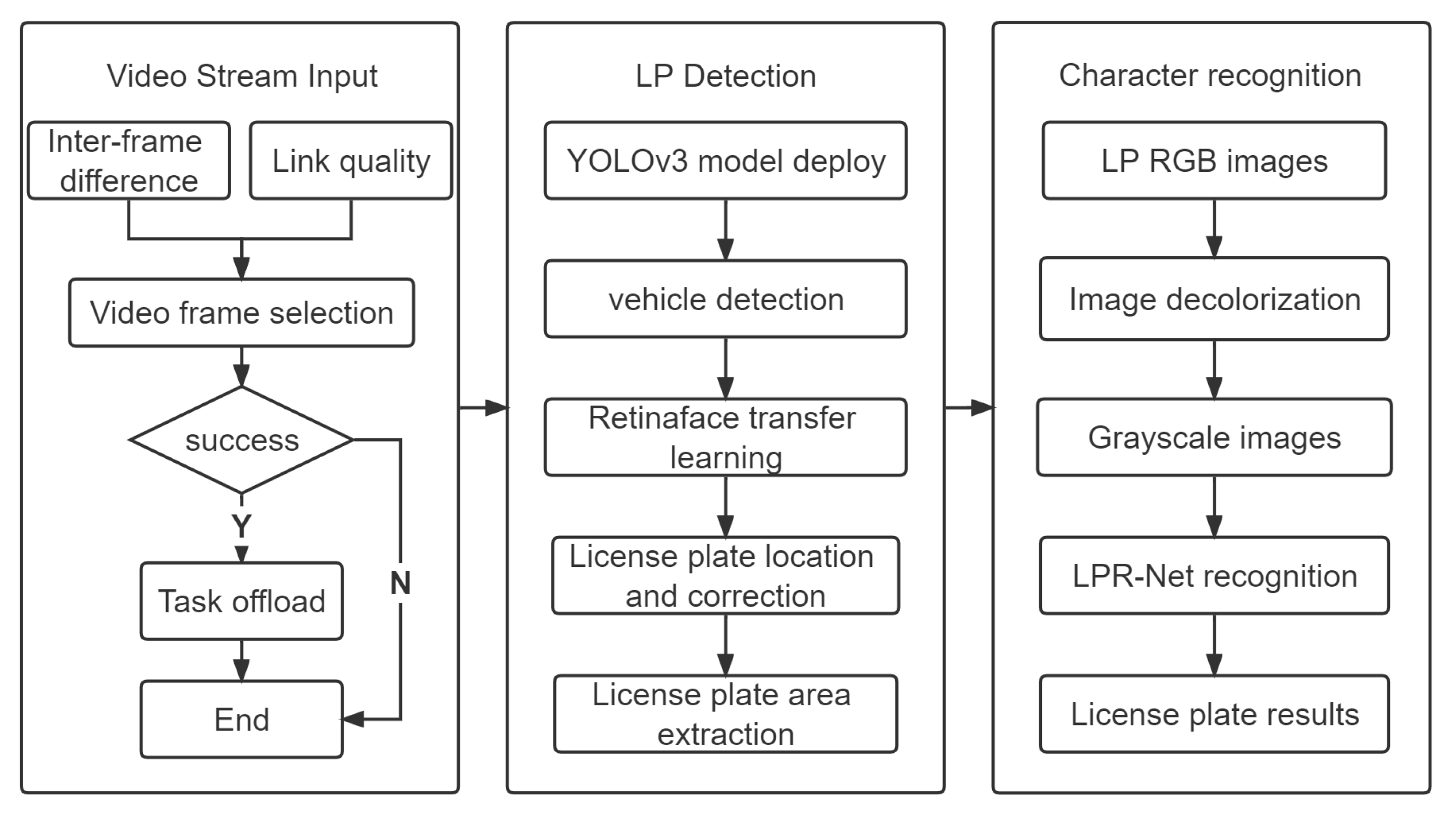
Figure 1. The System Framework of our edge-ALPR system.
Electronics 11 03186 g001
Figure 2. Schematic diagram of residual network of YOLOv3 algorithm.
Electronics 11 03186 g002
Figure 3. Comparison before and after the process of the image decolorization. (left) hu A. (right) hu A.
Electronics 11 03186 g003
Figure 4. The Flowchart of the proposed algorithm.
Electronics 11 03186 g004
Figure 5. Difference between frames, the white area shows fast movement and the black area shows slow movement.
Electronics 11 03186 g005
Figure 6. Diagram of Inter-frame difference and the corresponding symbolic expression.
Electronics 11 03186 g006
Figure 7. The workflow of edge-based ALPR system. Our proposed algorithms runs on the red rectangle part on IoT device.
Electronics 11 03186 g007
Figure 8. A series of test videos with different scenarios and different car number.
Electronics 11 03186 g008
Figure 9. Comparison of CASE 1, CASE 2 and CASE 5. (a) Variation in A c c u r a c y rate with different test video; (b) Variation in E x t r a c t i o n _ q u a l i t y rate with different test video.
Electronics 11 03186 g009
Figure 10. Comparison of CASE 1, CASE 3 and CASE 5. (a) Variation in A c c u r a c y rate with different test video; (b) Variation in E x t r a c t i o n _ q u a l i t y rate with different test video.
Electronics 11 03186 g010
Figure 11. Comparison of CASE 1, CASE 4 and CASE 5. (a) Variation in A c c u r a c y rate with different test video; (b) Variation in E x t r a c t i o n _ q u a l i t y rate with different test video.
Electronics 11 03186 g011
Figure 12. E n e r g y _ l o s s ( % ) comparison of CASE 1–5.
Electronics 11 03186 g012
Table 1. The existing four classic categories approaches for key frame extraction.
Category (Based on)Key IdeaLimitations
Video shot [27]Divides the video stream into several shots and then extracts the first frame, the middle frame and the last frame as key frames.(1) The number of key frames is limited as a fixed value.
(2) Complexity of content in the current video shot is not considered.
(3) The motion content cannot be efficiently described.
Motion analysis [28]Calculates the movement of a shot by analyzing the optical flow, selects the local minimum in the movement as key frames.(1) High calculation overhead.
(2) Poor robustness for content changes by dynamic accumulation.
Video content [29]Extracts key frames based on the change of color, texture and other visual information of each frame.(1) Unstable in scenarios when meet frequent camera or mass of content motion.
(2) Cannot indicate the changes quantitatively.
Clustering [30]Clusters into several clusters, and selects key frame from every cluster.(1) High calculation overhead.
(2) The number of cluster needs to be predefined.
Table 2. Back-bone network architecture [36] of the end-to-end deep learning network LPR-Net.
Layer TypeParameters
Input94 × 24 pixels image
Convolution#64 3 × 3 stride 1
MaxPooling#64 3 × 3 stride 1
Small basic block#128 3 × 3 stride 1
MaxPooling#64 3 × 3 stride (2, 1)
Small basic block#256 3 × 3 stride 1
MaxPooling#64 3 × 3 stride (2, 1)
Dropout0.5 ratio
Convolution#256 4 × 1 stride 1
Dropout0.5 ratio
Convolution# class_number 1 × 13 stride 1
Table 3. Some common application scenarios and corresponding parameters.
ScenariosV (km/h) FPS D (/m)
Highway60–12024–6030–60
Urban30–6024–6030–60
Street0–2524–6030–60
Parking lot entrance0–1024–603–6
Table 4. 20 times simulation results for one video in CASE 5 and average result.
IDKey Frame NumberTotal Time (/s)Single Time (/ms)All Cars? (YES/NO)Full Car FramesSuccess FramesAccuracy (/%)Extraction Quality (/%)
16350.67804YES555498.1887.30
28053.33666YES686697.0585.00
36148.05787YES535298.1186.88
46648.61736YES555498.1883.33
57552.08694YES646296.8785.33
68355.85673YES696695.6583.13
76951.01739YES575698.2482.60
88055.44693YES686697.0585.00
96149.15805YES535298.1186.88
108156.32695YES696695.6585.18
118355.47668YES696695.6583.13
126750.19749YES565598.2183.58
136552.07801YES545398.1483.07
147151.29722YES595898.3083.09
158356.07675YES696695.6583.13
168054.62682YES686697.0585.00
176348.17764YES535298.1184.12
187855.95717YES676698.5085.89
197051.31733YES585798.2782.85
208155.88689YES686697.0583.95
Average7352.5765724.6YES61.659.9597.40184.422
Publisher’s Note: MDPI stays neutral with regard to jurisdictional claims in published maps and institutional affiliations.