Abstract
This systematic review aims to provide deep insights on emerging trends in, and the potential of, advanced deep learning techniques, such as machine learning algorithms being partially replaced by deep learning (DL) algorithms for credit scoring owing to the higher accuracy of the latter. This review also seeks to explain the reasons that deep belief networks (DBNs) can achieve higher accuracy than shallower networks, discusses the potential classification capabilities of DL-based classifiers, and bridges DL and explainable credit scoring. The theoretical characteristics of DBNs are also presented along with the reasons for their higher accuracy compared to that of shallower networks. Studies published between 2019 and 2022 were analysed to review and compare the most recent DL techniques that have been found to achieve higher accuracies than ensemble classifiers, their hybrids, rule extraction methods, and rule-based classifiers. The models reviewed in this study were evaluated and compared according to their accuracy and area under the receiver operating characteristic curve for the Australian, German (categorical), German (numerical), Japanese, and Taiwanese datasets, which are commonly used in the credit scoring community. This review paper also explains how tabular datasets are converted into images for the application of a two-dimensional convolutional neural network (CNN) and how “black box” models using local and global rule extraction and rule-based methods are applied in credit scoring. Finally, a new insight on the design of DL-based classifiers for credit scoring datasets is provided, along with a discussion on promising future research directions.
1. Introduction
Appropriate customer selection is a key element of risk management in the banking industry [1]. However, achieving accuracy in risk assessment is considered a difficult task. In problems related to credit scoring, the dependent variable is dichotomous, where ‘0’ is assigned to failed loans and ‘1’ to non-failed loans. Thus, techniques such as logistic regression and neural networks (NNs) can be used to estimate the borrower’s probability of default [2]. To manage financial risks, banks collect information from customers and other financial institutions to distinguish safe borrowers from risky ones. However, current automated lending risk evaluation methods are imperfect, and the failure of credit scoring algorithms to accurately assess loan recipients can result in considerable losses. Thus, from the perspective of the banking sector, appropriate assessment of credit applicants is crucial.
The topic of credit scoring has been at the forefront in the fields of finance and economics in applying machine learning (ML) techniques such as decision trees (DTs) [3], NNs [4], and support vector machines (SVMs) [5]; thus, the performance of various classification algorithms for credit scoring has been intensively researched over the past 50 years. Initially, the accuracy gains of these methods (compared with the logistic regression model) for the assessment of creditworthiness appeared to be limited. However, the performance of ML-based scoring methods has improved considerably since the adoption of ensemble methods, especially bagging [6] and boosting [7] methods.
The application of deep learning (DL) to business analytics and operations has also attracted considerable research attention [8]. Kraus et al. [8] revealed that DL is a feasible and effective method in these fields and determined that it can outperform its traditional counterparts in terms of predictive accuracy. The development of accurate and analytical credit scoring models has thus emerged as a major area of focus for financial institutions [8]. Numerous classification algorithms have been proposed for credit scoring. For example, Gunnarsson et al. [9] reported that XGBoost, which was originally proposed by Chen and Guestrin [10], is the best-ranking classifier. However, the application of DL algorithms in credit scoring has been largely ignored in the literature [9].
DL has been successfully used in many real-world applications, especially in domains involving visual and audio recognition or time-series economic and financial data analysis. In these domains, the temporal and/or spatial correlation of data enables DL methods to learn features effectively, leading to superior classification results. DL models such as convolutional neural networks (CNNs) [11] and long short-term memory (LSTM) networks [12] commonly use data correlations to learn feature representations. One-dimensional (1D) CNNs have been applied to data with temporal correlations, such as stock indices, whereas convolution has been used to learn meaningful patterns in data. Existing DL methods largely benefit from this learning power to identify meaningful features by capturing temporal/spatial correlations [13]. In a systematic and comprehensive review, Sezer et al. [14] reported a lack of review papers focusing solely on DL for credit scoring, despite the growing interest in the development of models incorporating DL for financial time-series forecasting.
Furthermore, to the best of the author’s knowledge, only one review article on the application of DL to credit scoring has been published. Dastile and Celik [15] conducted a systematic literature survey on statistical and ML models for credit scoring to leverage the performance benefits of DL while complying with the legislation requirements for automated decision-making processes. In their paper, they briefly described the DL techniques in credit scoring published from 2015 to 2018, which represents the first trend of the replacement of statistical and classical ML techniques with DL techniques in credit scoring. Luo et al. [16] first used corporate default swap data to compare the performance of deep belief networks (DBNs) with that of logistic regression, multi-layer perceptrons (MLPs), and SVMs, and revealed that DBNs exhibited superior performance. Tran et al. [17] proposed a hybrid model combining genetic programming and stacked autoencoder (AE) network models. They compared the proposed hybrid model with logistic regression, k-nearest neighbor (KNN) classification methods, SVMs, artificial neural networks (ANNs), and DTs for credit scoring datasets. The results revealed that the proposed hybrid model exhibits excellent accuracy.
In a survey of the literature published from 2015 to 2018 on the use of DL for financial applications, Ozbayoglu et al. [18] described how relatively simple DL methods are for application in credit scoring. In addition, Yu et al. [19] proposed a unique cascade hybrid model of a DBN-based resampling SVM ensemble learning paradigm to classify the German and Japanese credit scoring datasets. However, over the past few years, novel DL-based methods for credit scoring have been rapidly developed.
As the present study aimed to provide an in-depth insight rather than a systematic review, studies published between 2019 and 2021 were searched using Web of Science, Science Direct, and IEEE eXplore. For Section 4 only, a few recent studies from arXiv were also selected. The present review focuses on an emerging trend in which ML techniques are partially being replaced by DL techniques for credit scoring. The architectures used in DL include DBNs [20], LSTM networks [12], CNNs [11], and AEs [21]. Such comparisons should be performed using a considerable number of real-world credit scoring datasets [8]. Thus, the models in this review were evaluated and compared in terms of their accuracy and area under the receiver operating characteristic curve (AUC) [22] for the Australian, German (categorical), German (numerical), Japanese, and Taiwanese datasets, which are commonly used in the credit scoring and other research communities [22]. Further, the improvements in accuracy and AUC values achieved with these datasets using ensemble classifiers and their hybrids, DL techniques, rule extraction, and rule-based classifiers for credit scoring have been tabulated as well.
Over 2019–2021, DL-based classifiers emerged as exhibiting the highest output accuracies, subsequently leading to the emergence of a “DL revolution” in credit scoring. A key aspect of DL-inspired ensemble systems involves the hierarchical distribution of ML elements in cascade and/or parallel ensembles [23,24,25]. Another key aspect is the conversion of tabular datasets into images using bins employed to calculate the weight of evidence (WOE) [26]. Dastile and Celik [27] considered both continuous and categorical features and achieved the highest accuracy (88%) amongst DL-based classifiers for the German (categorical) dataset.
The objectives of this review are fourfold: (1) to present certain theoretical characteristics of DBNs and the reasons they achieve higher accuracy than shallower networks with one hidden layer by using ML theorems; (2) to review the most recent DL techniques that have been shown to achieve higher accuracies than ensemble classifiers, their hybrids, rule extraction methods, and rule-based classifiers; (3) to reveal the potential classification capabilities of DL-based classifiers and investigate their applicability to credit scoring datasets; and (4) to provide deep insights into the usefulness and interpretability of DL in credit scoring and related financial areas.
The remainder of this paper is structured as follows. Section 2 presents the fundamentals of DL models used in credit scoring, such as deep multi-layer perceptrons (DMLPs), CNNs, LSTM networks, restricted Boltzmann machines (RBMs) [28], DBNs, AEs, discretised interpretable multi-layer perceptrons (DIMLPs), 1D CNNs, gcForest, and DL ensemble systems, as well as data attributes and preprocessing/encoding techniques for DL in credit scoring. Section 3 provides an overview of the accuracy, AUC, and methods recently reported for the Australian, German (categorical), German (numerical), Australian, and Taiwanese credit scoring datasets. Section 4 explains how the tabular datasets are converted into images for the application of a two-dimensional (2D) CNN over 2018–2021. Section 5 presents an explanation of “black box” models using local and global rule extraction and rule-based methods in credit scoring. Section 6 summarises the emerging trends and accuracies of various methods for the Australian, German (categorical), German (numerical), Australian, and Taiwanese datasets. Further, it highlights the potential capabilities of DL classifiers, discusses their applicability for credit scoring based on emerging trends reported mainly over 2020–2021 from the perspective of ML with and without DL techniques for the five datasets, outlines the design of CNN-based classifiers for credit scoring datasets, and provides promising research directions. Finally, Section 7 concludes the paper.
2. Fundamentals of Deep Learning Models Used in Credit Scoring
A DL model is a type of ML model that consists of multiple ANN layers and provides high-level abstraction for data modelling [29]. Up until now, various DL models have been reported in the literature, including DMLPs, CNNs, LSTM networks, RBMs, DBNs, AEs, DIMLPs, 1D CNNs, gcForest, and DL ensemble systems.
2.1. Previous Reviews
So far, two surveys related to the theme of this review have been published in the literature. The first [15] employed a systematic literature survey approach to systematically review statistical and ML models in credit scoring, identified limitations in the literature, and proposed a guiding ML framework. Although, this survey is well organised, it is based on journal and conference articles that were published between 2010 and 2018. Furthermore, although DL models had not been applied extensively in the credit scoring literature, they showed promising results that often were not fresh. Thus, the second survey [18] can be considered as the first comprehensive survey paper on “deep learning for financial applications”. Although it provides an excellent introduction to the basics of DL deep learning and is well-suited for understanding DL deep learning for broad financial applications, directly overlapped sections with the present review were limited to credit scoring and credit risk. In addition, although an original article [27], the sections contain a belief review of recent works in their Related Works section.
In contrast, the present review concentrates on articles published between 2019 and 2022, which correlated into the period of emergence of significant novel DL algorithms in credit scoring, as alluded earlier. This review was carried out based on the following four concepts: (1) whether the adoption of deep architectures (such as CNN [11] and XGBoost [10]) or shallow architectures (such as logistic regression) depends on the property of datasets; (2) classifier design and interpretability, such as rule extraction; (3) interchangeability between images and symbolic rules for classification; and (4) effectiveness of tabular image conversion for credit scoring.
2.2. Deep Multi-Layer Perceptrons (DMLPs)
DMLPs represent the first type of ANN models. They consist of input, output, and hidden layers, similar to an ordinary MLP; however, DMLPs have more layers.
2.3. Convolutional Neural Networks (CNNs)
CNNs, the first of which was proposed by LeCun et al. [11], constitute a type of deep neural network (DNN) mainly used for image classification and recognition problems. CNNs scan an entire image using filters. Most CNNs consist of numerous layers, such as convolutional layers based on convolution operation [18], subsampling or pooling (average or maximum) layers, and fully connected layers. The convolution operation extracts features from the data, whereas subsampling reduces data dimensionality. Compared with other NNs, CNNs exhibit weight sharing, pooling, and local connectivity, which is achieved by convolution and inspired by an image space in which the pixel correlation of relatively close pixels is strong, while that of faraway pixels is weak. A generalised CNN architecture is shown in Figure 1.
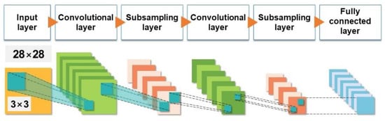
Figure 1.
Schematic overview of a generalised convolutional neural network. Source: Sezer et al. [14].
2.4. Long Short-Term Memory (LSTM) Networks
LSTM networks [12] are DL networks specifically designed for sequential data analysis. An advantage of LSTM networks is that both short- and long-term values in the network can be remembered. Therefore, they are mainly used for sequential data analysis (e.g., speech recognition, time-series data). LSTM networks consist of LSTM units. Each LSTM unit consists of cells with input, output, and forget gates that regulate the information flow. These features enable each cell to remember the desired values over arbitrary time intervals. LSTM cells combine to form layers of NNs [16]. The schematic of a basic LSTM unit is shown in Figure 2.
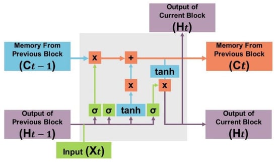
Figure 2.
Schematic of a long short-term memory network (σ: sigmoid function, tanh: hyperbolic tangent function, X: multiplication, +: addition). Source: Sezer et al. [14].
2.5. Restricted Boltzmann Machines (RBMs)
RBMs are bipartite, undirected, graphical ANN models that consist of two layers—a visible layer and a hidden layer—that can learn the probability distribution of an input set [28] and are mainly used for dimension reduction, classification, and feature-learning. Each unit makes stochastic decisions to determine whether the input data should be transmitted, and the units in the layers are not connected to each other. Each cell is a computational point that processes the input. A graphical overview of an RBM is shown in Figure 3.
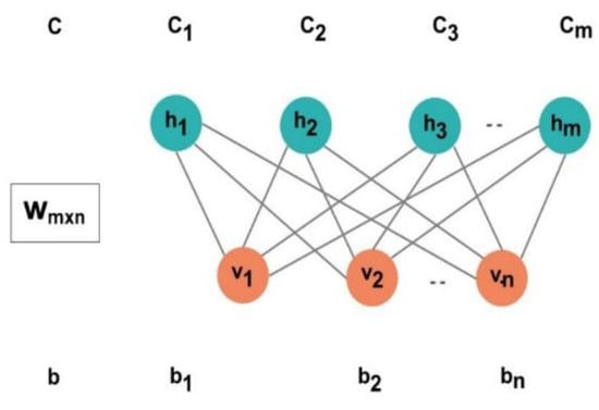
Figure 3.
Schematic of a restricted Boltzmann machine. Source: Sezer et al. [14].
2.6. Deep Belief Networks (DBNs)
DBNs [20] are ANNs that consist of a stack of RBM layers. They are probabilistic generative models that include latent variables and are used for determining independent and discriminative features in an input set by using an unsupervised approach. After DBNs learn to reconstruct the input set probabilistically during the training process, the layers in the network begin to detect the discriminative features. After this learning step, supervised learning is performed for classification. The structure of a DBN is shown in Figure 4.
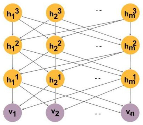
Figure 4.
Schematic of a deep belief network. Source: Sezer et al. [14].
2.7. Autoencoders (AEs)
Typically, AE networks [21] are used in DL models to remap the inputs (features) such that they are more representative for classification. Thus, AE networks perform unsupervised feature-learning. A representation of a dataset is learned through dimensionality reduction using an AE, which are typically used for feature extraction and dimension reduction. They include an input layer, output layer, and one or more hidden layers that connect the layers together. The number of nodes in the input layer is equal to the number of nodes in the output layer, and they exhibit a symmetrical structure. AEs consist of two components, namely an encoder and a decoder. The basic structure of an AE is shown in Figure 5.
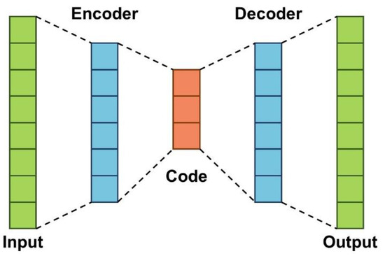
Figure 5.
Schematic of an autoencoder. Source: Sezer et al. [14].
2.8. Discretised Interpretable Multi-Layer Perceptrons (DIMLPs)
DIMLPs differ from MLPs in terms of the connectivity between the input layer and the first hidden layer. Specifically, a hidden neuron receives only a connection from an input neuron and a bias neuron. After the first hidden layer, the neurons are fully connected. Notably, DIMLPs consist of two hidden layers, with the number of neurons in the first hidden layer equal to that of the input neurons [30].
2.9. One-Dimensional Convolutional Neural Networks (1D CNNs)
Typically, 2D CNNs are preferred over 1D CNNs. Therefore, CNNs are not the first choice for analysing credit scoring datasets, which contain categorical attributes. Hayashi and Takako [31] used a combination of a 1D fully connected layer first CNN (1D FCLF-CNN [32]) and the recursive-rule extraction algorithm with J48graft [33] to develop a novel approach for achieving transparency and conciseness in credit scoring datasets with heterogeneous attributes. In their network, first, the input layer is connected to a number of fully connected layers, followed by a typical CNN. By adding a Softmax layer, the fully connected layers before the convolutional layers in a 1D FCLF-CNN (Figure 6) are regarded as encoders; this provides a better local structure that can transfer raw instances into representations because structured datasets are similar to disrupted image data, which appear to exhibit no local structure. An inception module [34] was used to construct the 1D FCLF-CNN.
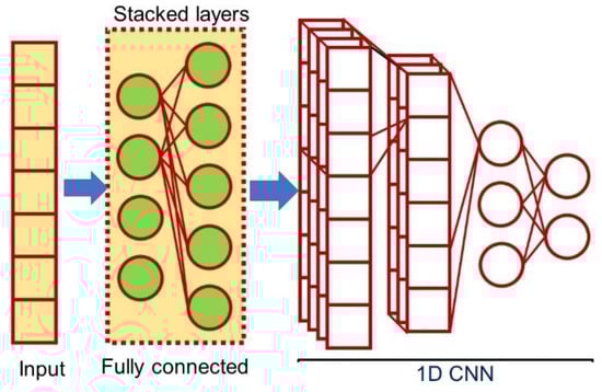
Figure 6.
Schematic of a one-dimensional fully connected layer first convolutional neural network.
2.10. gcForest
To improve the learning ability and classification performance of a model, Zhou and Feng [35,36] proposed gcForest (Figure 7), a tree-based ensemble method that uses a cascade structure to process features in a layer-by-layer manner. In gcForest, to reduce the risk of overfitting, the class vector is generated by each forest in the cascade structure through k-fold cross-validation. Although gcForest achieved comparable performance with that of DNNs in a number of tasks and has performed well in many fields, it has not yet been applied to credit scoring.
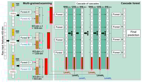
Figure 7.
Schematic overview of the main part of gcForest. Source: Zhou and Feng [35,36].
2.11. Deep-Learning-Inspired Ensemble Systems
The deep genetic hierarchical network of learners (DGHNL) methodology, which consists of a fusion-based 29-layer structure, including feature extraction approaches, 5 ML algorithms, kernel functions, and both normalisation and parameter optimization techniques, was introduced by Pławiak et al. as an extension of their previous work [23,24]. Their main motivation for developing DGHNL was to boost the performance of credit scoring prediction systems by applying an ensemble learning technique with many layers, as the performance of classical ML methods can be enhanced by the application of evolutionary algorithms [24]. A schematic of DGHNL is shown in Figure 8.
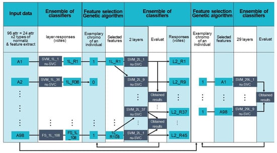
Figure 8.
Schematic overview of the main part of the deep genetic hierarchical network of learners. Source: Pławiak et al. [23].
2.12. Types of Data Attributes
The number of cases with more than one type of attribute in a supervised control architecture has increased considerably [37]. Categorical attributes consist of two subclasses—nominal and ordinal—with the ordinal subclass inheriting certain properties of the nominal. Similar to nominal attributes, all categories (i.e., possible values) of the attributes in ordinal data (i.e., the data associated with only ordinal attributes) are qualitative and unsuitable for mathematical operations. However, the attributes are naturally ordered and comparable [38], for example, in a dataset related to individuals containing a numerical attribute, such as 0.567, 78.9, 10, or 100, an ordinal attribute such as a Stage I, II, or III cancer diagnosis, and a nominal attribute, such as university student, public employee, company employee, lawyer, teacher, or professor [39].
2.13. Weights of Evidence
Certain classification algorithms (e.g., classification trees, Bayes classifiers) are well-suited to data of mixed scaling levels, whereas others (e.g., ANNs, SVMs) benefit from encoding nominal variables. Thomas and Edelman [26] suggested two methods of evaluating the categorical variables for loan evaluations. The first is the creation of binary dummy variables for each possible value of an attribute, and the second avoids the creation of numerous dummies by performing WOE encoding. For each attribute value, the numbers of good and bad risks are counted, and the WOE is calculated as follows:
where p(value = good) is the number of good risks that have this value for the attribute divided by the total number of good risks, and p(value = bad) is the number of bad risks having this value for the attribute divided by the total number of bad risks. The categorical answers are replaced by these weights of evidence, with higher weights indicating that the attribute value corresponds with good risks.
2.14. Limitations on the Availability of Datasets
The datasets used in this review are very old and small in size (690–1000 instances). Because they are small, DL methods might not achieve good performance. The Kaggle credit dataset (https://www.kaggle.com/c/GiveMeSomeCredit/data, accessed on 10 January 2020) contains 250 K instances, and recent papers have used datasets that are even larger; however, often, these data are not publicly available.
3. Review of Recent Deep Learning Techniques in Credit Scoring
In this section, the performance of recent ensemble and hybrid classifiers for the Australian (Table 2), German (categorical) (Table 3), German (numerical) (Table 4), Japanese (Table 5), and Taiwanese (Table 6) credit datasets is first tabulated. Then, the performance of recent DL techniques for these five credit datasets is reviewed.
3.1. Credit Scoring Datasets
In this subsection, the characteristics of the Australian, German (categorical), German (numerical), Japanese, and Taiwanese datasets (Table 1) are described, each of which exhibits a distinct imbalance ratio. Five credit datasets with distinct imbalance ratios were used to review the performance of DL techniques for credit scoring. These datasets were obtained from the UCI ML Repository (https://archive.ics.uci.edu/ml/index.php) and are easily accessible.

Table 1.
Characteristics of the five credit datasets.
3.2. Area under the Receiver Operating Characteristic Curve (AUC)
To define AUC, let us introduce the true negative (TN), false positive (FP), false negative (FN), and true positive (TP). For credit scoring classification, TN represents the number of borrowers who are correctly classified as non-defaults, FP represents the number of defaulted borrowers who are incorrectly classified as defaults, FN represents the number of defaulted borrowers who are incorrectly classified as non-defaults, and TP represents the number of borrowers who are correctly classified as defaults [15]. Thus, AUC, which measures the discriminative power of model between classes [22], is calculated as per the following equation:
3.3. Performance of Various Classification Techniques
As the performance of classifiers in aspects such as predictive accuracy differs considerably with or without DL techniques, these performance parameters were investigated separately.
3.4. Deep Learning Models Used in Credit Scoring
This section investigates various DL models applied in credit scoring research. DL models are categorised according to their function into five subcategories: discriminative, representative, generative, ensemble, and hybrid DL models, as shown in Figure 9.
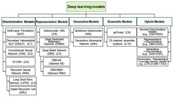
Figure 9.
Taxonomy of deep learning models applied to credit scoring.
3.4.1. Performance of Classifiers without Deep Learning Techniques
The accuracy and AUC values of both ensemble and hybrid classifiers without DL techniques, which are considered conventional classifiers, for the Australian dataset are shown in Table 2. Employing a clustering-based financial risk assessment model, Acharya [40] proposed a novel wrapper feature selection approach. Initially, the features were ranked using an information-gain-directed feature selection (IGDFS) algorithm, and the highest-ranking n features were propagated using a genetic algorithm-based wrapper (GAW) model. The data generated from the previous stage were then clustered using an improved k-means clustering technique. When this clustering process was completed, the data were classified using a gradient-boosting tree (GBT) classifier model. The incorporation of the IGDFS, GAW, and GBT models achieved the highest accuracies for the Australian and German datasets (98.98% and 98.66%, respectively).
Table 2.
Accuracy and area under the receiver operating characteristic curve (AUC) values of ensemble and hybrid classifiers for the Australian dataset.
Table 2.
Accuracy and area under the receiver operating characteristic curve (AUC) values of ensemble and hybrid classifiers for the Australian dataset.
| Authors (Year) [Ref.] | Accuracy (%) | AUC | Methods |
|---|---|---|---|
| Acharya et al. [40] | 98.98 | ----- | IGDFS + gradient boosting tree (GBT) classifier |
| Kuppili et al. (2020) [41] | 95.58 | 0.97 | Spiking extreme learning machines |
| Tripathi et al. (2018) [42] | 95.39 | Neighborhood rough set (NRS) + ML ensemble | |
| Radović et al. (2021) [43] | ----- | 0.92 | Ensemble classifier |
| Hsu et al. (2018) [44] | 92.75 | ---- | Artificial bee colony-based SVM |
| Tripathi et al. (2019) [45] | 92.69 | ---- | Ensemble feature selection + ML ensemble |
| Edla et al. (2018) [46] | 92.58 | ---- | Binary particle swarm optimization and gravitational search algorithm (BPSOGSA) |
| Zhang et al. (2021) [47] | 92.36 | 0.965 | Multi-stage ensemble |
| Tripathi et al. (2020) [48] | 89.92 | 0.953 | Evolutionary extreme learning machine |
| Xu et al. (2020) [49] | 89.5 | 0.937 | Extreme learning machine (ELM) and generalized fuzzy soft sets (GFSS) |
| Li et al. (2021) [50] | 88.55 | 0.945 | Two-stage hybrid default discrimination model based on deep forest |
| Xu et al. (2018) [51] | 88.1 | 0.935 | GFSS |
| Zhang et al. (2018) [52] | 87.61 | 0.933 | Classifier selection and clustering |
Kuppili [41] achieved the second-highest accuracy (95.58%) using spiking extreme learning machines, which have also been shown to be effective for credit score classification. A novel spike-generating function was proposed in the leaky nonlinear integrate and fire model. Its interspike period was computed and then used in an extreme learning machine for credit score classification. To improve classification performance, Tripathi et al. [42] proposed the use of a hybrid credit scoring model based on dimension reduction using the neighborhood rough set (NRS) algorithm along with layered ensemble classification and the weighted voting approach.
Trivedi [43] achieved the second-highest accuracy (93.12%) for the German (categorical) dataset by comparing three feature selection techniques and five ML classifiers and revealed that the chi-square feature selection method was suitable with the most informative predictors for all ML models. (Table 3). The random forest (RF) method was the best amongst the other ML classifiers. A limitation of that study is that only the German (categorical) dataset was considered. However, it provided sufficient scope to test other credit datasets using the identified prediction model.
Table 3.
Accuracy and area under the receiver operating characteristic curve (AUC) values of hybrid and ensemble classifiers for the German (categorical) dataset.
Table 3.
Accuracy and area under the receiver operating characteristic curve (AUC) values of hybrid and ensemble classifiers for the German (categorical) dataset.
| Authors (Year) [Ref.] | Accuracy (%) | AUC | Methods |
|---|---|---|---|
| Acharya et al. [40] | 98.66 | ---- | IGDFS + GBT classifier |
| Trivedi (2020) [53] | 93.12 | ----- | Feature selection + ML classifier selection |
| Tripathi et al. (2018) [42] | 86.47 | ----- | NRS + ML ensemble |
| Edla (2018) [46] | 85.78 | ----- | Hybrid binary particle swarm optimization and gravitational search algorithm (BPSOGSA) |
| Hsu et al. (2018) [44] | 84.0 | ------ | Artificial bee colony-based SVM |
| Arora et al. (2020) [54] | 84.0 | 0.713 | Bolasso-based feature selection |
| Yu et al. (2009) [55] | 82.0 | 0.824 | Fuzzy group decision-making (GDM) |
| Zhang et al. (2020) [56] | ---- | 0.684 | Heterogeneous ensemble |
| Radović et al. (2021) [43] | ----- | 0.77 | Ensemble classifiers |
| Zhang et al. (2021) [47] | 79.5 | 0.831 | Multi-stage ensemble |
Xu et al. [54] reported a hybrid data mining ensemble learning classification algorithm for the generalized fuzzy soft sets (GFSS) theory and achieved the second-highest accuracy (87.6%) and AUC (0.813) for the German (categorical) dataset (Table 4).
Table 4.
Accuracy and area under the receiver operating characteristic curve (AUC) values of hybrid and ensemble classifiers for the German (numerical) dataset.
Table 4.
Accuracy and area under the receiver operating characteristic curve (AUC) values of hybrid and ensemble classifiers for the German (numerical) dataset.
| Authors (Year) [Ref.] | Accuracy (%) | AUC | Methods |
|---|---|---|---|
| Song and Peng (2019) [57] | ------ | 0.961 | MCDM-based evaluation approach |
| Tripathi et al. (2021) [58] | 88.24 | ----- | DNN (Time Delay Neural Network) |
| Xu et al. (2019) [50] | 87.6 | 0.813 | GFSS |
| Tripathi et al. (2020) [48] | 80.57 | 0.862 | ELM + novel activation function |
| Wang et al. (2018) [59] | 78.53 | ----- | Hybrid approach based on filter approach and multiple population GA |
| Lappas et al. (2021) [60] | ----- | 0.789 | ML + expert knowledge with GA |
| Liu et al. (2021) [61] | 77.15 | 0.792 | Step-wise multi-grained augmented boosting DT |
Zhang et al. [47] proposed a novel multi-stage ensemble model with enhanced outlier adaption and achieved the highest accuracy (93.16%) for the Japanese dataset. (Table 5). To reduce the adverse effects of outliers existing in the noise-filled credit datasets, a local outlier factor algorithm was enhanced using the bagging strategy to identify outliers effectively and boost them back into the training set to construct an outlier-adapted training set that enhanced the outlier adaptability of the base classifiers.
Table 5.
Accuracy and area under the receiver operating characteristic curve (AUC) values of hybrid and ensemble classifiers for the Japanese dataset.
Table 5.
Accuracy and area under the receiver operating characteristic curve (AUC) values of hybrid and ensemble classifiers for the Japanese dataset.
| Authors (Year) [Ref.] | Accuracy (%) | AUC | Methods |
|---|---|---|---|
| Zhang et al. (2021) [47] | 93.16 | 0.969 | Multi-stage ensemble with enhanced outlier adaption |
| Tripathi et al. (2021) [58] | 90.44 | ----- | Time Delay Neural Network (TDNN) |
| Chen et al. (2021) [62] | 89.64 | 0.914 | Generalized Shapley–Choquet integral (GSCI)-based ensemble approach |
| Xu et al. (2019) [49] | 89.4 | 0.933 | GFSS |
| Tripathi et al. (2021) [48] | 88.35 | 0.946 | Evolutionary ELM |
Tripathi et al. [58] performed a comparative result analysis to assess the impact of feature section and classification approaches that combine feature selection with a classifier. They reported that the ensemble classifier-based feature selection with KNN achieved the highest accuracy (89.44%) for the Taiwanese dataset (Table 6).
Table 6.
Accuracy and area under the receiver operating characteristic curve (AUC) values of hybrid and ensemble classifiers for the Taiwanese dataset.
Table 6.
Accuracy and area under the receiver operating characteristic curve (AUC) values of hybrid and ensemble classifiers for the Taiwanese dataset.
| Authors (Year) [Ref.] | Accuracy (%) | AUC | Methods |
|---|---|---|---|
| Tripathi et al. (2021) [58] | 89.44 | ----- | KNN + Feature selection |
| Liu et al. (2021) [61] | 87.08 | 0.936 | Step-wise multi-grained augmented boosting DT |
| Zhang et al. (2021) [47] | 82.93 | 0.809 | Multi-stage ensemble with enhanced outlier adaption |
| Sariannidis et al. (2000) [63] | 82.65 | ----- | Decision-making based on machine learning |
| Li et al. (2021) [50] | ----- | 0.827 | Feature transformation + ensemble model |
3.4.2. Performance of Classifiers with Deep Learning Techniques
Pławiak et al. [23] proposed an SVM deep genetic cascade ensemble classifier (DGCEC) based on evolutionary computation, ensemble learning, and DL for the Australian dataset and achieved the highest accuracy (97.39%; see Table 7). Metawa [25] proposed a new type of feature selection using elephant herd optimization (EHO) with the DBN-modified water wave optimization (MWWO) algorithm for financial credit prediction. The EHO algorithm was used as a feature selector and MWWO–DBN for classification. The MWWO–DBN method achieved an accuracy of 94.2% for the Australian dataset. Currently, DL techniques have exhibited better results (97.39%) than expected, comparable to the highest accuracy (98.98%) achieved by Acharya et al. [40] using IGDFS and GBT models.
Table 7.
Accuracy and area under the receiver operating characteristic curve (AUC) values of deep-learning-based classifiers for the Australian dataset.
Table 7.
Accuracy and area under the receiver operating characteristic curve (AUC) values of deep-learning-based classifiers for the Australian dataset.
| Authors (Year) [Ref.] | Accuracy (%) | AUC | Methods |
|---|---|---|---|
| Pławiak et al. (2019) [23] | 97.39 | ---- | DL ensemble systems |
| Metawa et al. (2021) [25] | 94.2 | ---- | Elephant herd optimization (EHO) with modified water wave optimization (MWWO)-based DBN |
| Li et al. (2021) [52] | 88.55 | 0.942 | Two-stage hybrid default discriminant model based on deep forest |
| Liu et al. (2021) [63] | 88.26 | 0.940 | Multi-layered gradient boosting decision tree |
| Jiao et al. (2021) [64] | 84.72 | ---- | CNN-XGBoost |
Table 8 summarises the accuracy and AUC values of DL techniques in credit scoring for the German (categorical) dataset. Currently, only two DL techniques have been proposed for the German (categorical) dataset. This is likely because classifying the German (categorical) dataset using DL techniques is more difficult than classifying the German (numerical) dataset.
Table 8.
Accuracy and area under the receiver operating characteristic curve (AUC) values of deep-learning-based classifiers for the German (categorical) dataset.
Dastile et al. [27] achieved an accuracy of 88.0% by converting tabular datasets into images for a CNN. The accuracy for the German (categorical) dataset obtained by Dastile et al. [27] was considerably higher than that obtained by Li [50] (81.2%). Although this accuracy was lower than that of Acharya et al. [40], Dastile et al. [27] first achieved an accuracy of 88% by innovatively converting tabular datasets into images. The details of their conversion methods are covered in Section 4.
Li et al. [50] constructed a two-stage hybrid default discrimination model based on multiple feature selection methods and gcForest. Their proposed hybrid method provides the advantages of not only traditional statistical models, in terms of interpretability and robustness, but also DL models, in terms of accuracy. They achieved an accuracy of 81.2% for the German datasets.
Pławiak et al. [24] proposed a novel DGHNL model with a 29-layer structure (Figure 8) and achieved an accuracy of 94.60% for the German dataset (numerical; 24 attributes) with all numerical and no nominal attributes. However, because this dataset had no nominal attributes, it could be easily classified. Therefore, this fundamentally differs from the other German dataset (categorical; 20 attributes).
Shen et al. [65] developed a new DL ensemble model to evaluate credit risk and address imbalanced credit data. First, an improved synthetic minority oversampling technique [66] was designed to overcome the shortcomings of the original oversampling technique; after this, a novel DL ensemble classification method combined with an LSTM network and the adaptive boosting (AdaBoost) [67] algorithm was developed to train and learn the processed credit data. The proposed algorithm achieved an AUC value of 0.803 for the German (numerical) dataset (see Table 9).
Table 9.
Accuracy and area under the receiver operating characteristic curve (AUC) values of deep-learning-based classifiers for the German (numerical) dataset.
Jiao et al. [64] used the CNN-XGBoost model with adaptive particle swarm optimization (APSO) [68] to develop a credit scoring model and investigate classification performance. First, to eliminate the errors caused by data with self-variations or large differences in values, they preprocessed the original credit data. Next, they performed feature engineering to extract the most useful features from the original data. Finally, the model was developed with the selected features, the optimised hyperparameters were tuned using APSO, and test data tokens were used to evaluate the trained models. The proposed model achieved better results for credit scoring datasets.
Liu et al. [61] reported an accuracy of 68.75% and an AUC of 0.746 for the Taiwanese dataset using DF, a hierarchical multi-layered RF that can be considered as another multi-layered tree-based framework that realises representation learning [35,36]. In addition, Liu et al. [61] proposed an enhanced multi-layered gradient boosting decision tree for credit scoring that leverages the robustness of ensemble approaches (see Table 10 and Table 11), the feature enhancement of multi-grained scanning, and the representation learning ability of deep models.
Table 10.
Accuracy and area under the receiver operating characteristic curve (AUC) values of deep-learning-based classifiers for the Japanese dataset.
Table 11.
Accuracy and area under the receiver operating characteristic curve (AUC) values of deep-learning-based classifiers for the Taiwanese dataset.
4. Converting Tabular Datasets into Images to Apply Two-Dimensional Convolutional Neural Networks (2D CNNs)
DL differs from conventional ML because it can learn good feature representation from data. Existing DL methods greatly benefit from this feature-learning ability to determine meaningful features to capture temporal/spatial correlations [13].
In practice, in conventional ML and data classification, a different setting is considered in which instances are assumed to be independent and identically distributed, while features used to represent data are assumed to have weak or no correlations. Because of this assumption, conventional ML methods do not consider feature/data correlations in the learning process. Most conventional ML methods, including multi-layer NNs and randomised learning methods, such as stochastic configuration networks, do not explicitly consider feature interactions for learning, mainly because they require feature correlations to be handled via a data preprocessing method that creates independent features before applying the ML methods.
Neagoe et al. [69] compared deep CNNs and MLPs using credit scoring datasets and reported that deep CNNs achieved higher accuracy for the German and Australian datasets. However, according to Hamori et al. [70], the DL model performance depends on the choice of the activation function, the number of hidden layers, and the dropout rate. Their results showed that ensemble methods such as boosting and bagging achieve better performance on the Taiwanese credit scoring dataset compared to DNNs. These studies suggest the applicability of CNNs to credit scoring datasets.
Zhu et al. [71] used a hybrid method to perform credit scoring by combining a CNN with a relief algorithm (to perform feature selection) and found that this hybrid relief–CNN model achieved better performance than logistic regression and RF [72]. It converted tabular credit scoring data into images by bucketing and mapping features into image pixels. However, in their study, they considered numerical features only. As a result, their relief–CNN hybrid model outperformed benchmark models such as logistic regression and RF for credit scoring.
Inspired by the Super Characters method and 2D embeddings, Sun et al. [73] proposed the SuperTML method to address the problem associated with classifying tabular data. In their method, for each input, the features are first projected into 2D embeddings, such as an image, and then this image is fed into fine-tuned 2D CNN models for classification. A conceptual example of SuperTML is shown in Figure 10.
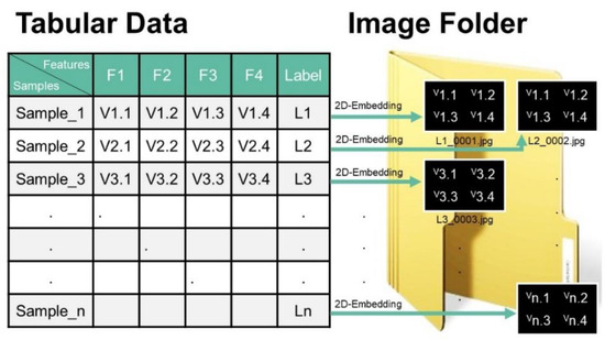
Figure 10.
Example of classification of tabular data. Source: Sun et al. [73].
Han et al. [13,66,74] proposed using DL for generic data classification, a technique in which rows of data are transformed from tabular into matrix form for use as inputs to CNNs. However, using CNNs to classify tabular data has progressed slowly. As a result, the use of non-NN methods, including SVMs and XGBoost, is still predominant for working with tabular data.
Buturović and Miljković [75] developed a tabular convolution approach to convert tabular datasets into images by treating each row of tabular data (i.e., feature vector) as an image filter (kernel) and then applying that filter to a fixed base image for application in 2D CNN models. A CNN was then trained to classify these filtered images. In their study, they used gene expression data obtained from the blood of patients with bacterial or viral infection.
In most tabular data, the spatial relationships between features are not considered and are therefore unsuitable for modelling using CNNs. To overcome this challenge, Zhu et al. [76] developed a novel image generator to convert tabular data into images by assigning features to pixel positions such that similar features are close to each other. Their algorithm obtains an optimised assignment by minimising the difference between the ranking of distances amongst features and the ranking of distances amongst their assigned pixels.
Using CNNs, Sharma and Kumar [77] proposed a new data-wrangling preprocessing method that can transform a 1D data vector into a 2D graphical image with appropriate correlations amongst fields. To our knowledge, for non-time-series data, this is the first method capable of converting non-image data to image data. These converted data, which are processed using a CNN with VGGnet-16, achieved competitive classification accuracy results compared with the canonical ANN approach; this suggests that there is considerable potential for further improvement of the method.
5. Explanation and Interpretation of the “Black Box” of Deep-Learning-Based Classifiers in Credit Scoring
5.1. Rule Extraction and Rule-Based Methods in Deep-Learning-Based Classifiers
Gunnarsson et al. [9] revealed that DBNs can be considered “black box” models; if the interpretability of the model’s prediction is the main concern, one must explain and interpret the “black box” model of DNNs through DL in credit scoring. Rule extraction from DNNs has also been summarised [78], and investigations on rule extraction methods have been carried out to balance interpretability and predictive performance. The core strategy of rule extraction methods is to construct a transparent “white box” model, such as a rule-based model or a decision tree, based on opaque “black box” models. A “white box” model is more suitable for understanding the reason behind high-stakes decisions. In addition, by analysing the “white box” model, the decision-makers can indirectly explain the “black box” model [79].
A comprehensive survey on local interpretation methods for DBNs has been carried out based on published works from 2012 to 2021. Another study proposed a novel rule extraction method for improving the ensemble model by balancing predictive performance and interpretability in two stages: a local rule extraction method followed by global rule extraction [80].
Another study proposed a new type of explanation that directly measures the interaction effects of local features and a new set of tools for understanding global model structures by combining multiple local explanations of each prediction [81]. Global approaches are increasingly being adopted over local approaches to explain the decisions of “black box” classifiers for a single instance.
Setzu et al. [82] addressed this problem by adding an interpretable layer on top of “black box” models by aggregating “local” explanations. They proposed GLocalX, an agnostic “local-first” model explanation method. Starting from local explanations expressed in the form of local decision rules, GLocalX iteratively generalises them into global explanations through hierarchical aggregation. Dong et al. [79] proposed two-stage rule extraction based on a tree ensemble model for interpretable loan evaluation.
5.2. Performance of Rule-Based Classifiers and Rule Extraction Methods for Credit Scoring
The performance of rule-based classifiers and rule extraction methods for the Australian and German credit scoring datasets are summarised in Table 12, Table 13 and Table 14, respectively. Generally, these methods exhibited excellent performance figures. Notably, the approach proposed by Soui et al. [83] achieved the best accuracy (94%), with 4.8 rules (averaged) for the Australian dataset, and an accuracy of 92.3% with 5.1 rules (averaged) for the German dataset, indicating its high accuracy and conciseness. By contrast, previous studies [31,32] have been subject to “no free lunch” (NFL) limitations [84,85] or the accuracy–interpretability dilemma; the method proposed by Soui et al. [83] mostly overcomes these barriers.
Table 13.
Performance of rule extraction methods and rule-based classifiers for the German (categorical) dataset.
Table 14.
Performance of deep-learning-based classifiers on the German (numerical) dataset.
Table 12.
Performance of rule extraction methods and rule-based classifiers for the Australian dataset.
Table 12.
Performance of rule extraction methods and rule-based classifiers for the Australian dataset.
| Authors (Year) [Ref.] | Accuracy (%) | AUC | # Rules | Methods |
|---|---|---|---|---|
| Soui et al. (2021) [83] | 94 | 0.92 | 4.8 | Multi-objective particle swarm optimization (SMOPSO) |
| Giri et al. (2021) [86] | ----- | 0.927 | 19.0 | Locally and globally tuned biogeography-based rule-miner (LGBBO-Miner) |
| Dong et al. (2021) [79] | ---- | 0.91 | 11.6 | Local rule extraction and global rule extraction |
| Hayashi and Oishi (2018) [87] | 88.4 | 0.87 | 14.1 | Sequential ensemble |
| Yedjour (2020) [88] | 87.41 | 6.12 | MNNGR | |
| Hayashi and Takano (2020) [32] | 86.53 | 0.871 | 2.6 | 1D LFCF-CNN with J48graft |
| Bologna and Hayashi (2018) [31] | 86.5 | 21.4 | DIMLP |
6. Discussion
6.1. Data Science (DS) and Machine Learning (ML) Classifiers
In DS, data are categorised into structured (also known as “tabular data”) and unstructured data. Currently, DNN models are widely applied for unstructured data such as images, speech, and text. However, there is no reason to believe that CNNs are definitely adopted for structured data such as tabular and credit scoring data.
ML models such as SVMs, GBT models, RF, and logistic regression have been used to process structured data. According to the 2020 Kaggle ML and DS Survey, a subdivision of structured data, known as relational data, is the most popular type of data in the industry, used by at least 70% of companies in their daily operations. Regarding structured data competitions, the CEO of Kaggle revealed that XGBoost is currently winning almost every competition in the structured data category. Therefore, form a practical perspective, XGBoost is the best choice, which is in accordance with a previous study [9]. Conversely, these facts suggest that there is huge potential to adopt DL-based classifiers for not only credit scoring datasets but also various business analytics datasets.
6.2. Applicability of Deep Belief Networks (DBNs) for Credit Scoring Based on ML Theorems
Gunnarsson et al. [9] concluded that deep networks with several hidden layers, namely DBNs, do not outperform shallower networks with one hidden layer. This phenomenon has been explained as follows. DBNs are subject to NFL limitations [84,85]. Although DL models perform well with images that have low abstraction data, they do not provide satisfactory results for images with higher abstraction data [86]. An empirical overview of DNNs reported disappointing results for simple and small data [87]. The models could not produce satisfactory results because of the limited number of datasets and, possibly, the low potential for data abstraction. These results are in accordance with previous findings [9].
However, Gómez and Rojas [87] claimed that although DBNs are subject to NFL limitations, exceptions regarding the number of hidden layers in DBNs exist for the limited number of datasets and, possibly, the low potential for data abstraction. Another study attempted to overcome these limitations by obtaining a limited number of hidden layers (one or two) in the DBN with consistently high accuracy [88]. These phenomena are in accordance with a discussion on the representational power of DBNs, and the best result achieved on switching from one- to two-layer DBNs was unexpected [89]. This result could be attributed to universal approximations [90] by RBMs, as credit scoring datasets do not require many RBMs or hidden units.
6.3. Accuracy of Deep-Learning-Based Classifiers in Credit Scoring
6.3.1. Accuracy of Deep-Learning-Based Classifiers in Credit Scoring for the Australian Dataset
As shown in Figure 11, two DL-based classifiers are present amongst the top five classifiers with the highest accuracy and a rule-based method is present in the top ten for the Australian dataset. The DL-based classifiers provide tough competition to the best ML classifier. The DGCEC proposed by Pławiak et al. [24] achieved the second-highest accuracy (97.39%), while the MWWO–DBN method proposed by Metawa et al. [25] achieved an accuracy of 94.2% for the Australian dataset.
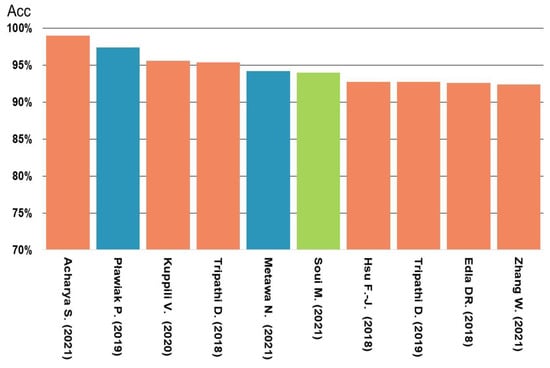
Figure 11.
Comparison of accuracy of various methods for the Australian dataset [23,25,40,41,42,44,45,46,47,83].
6.3.2. Tradeoff Curve between Accuracy and Interpretability for the German (Categorical) Dataset
Figure 12 shows the comparative results for the classification of the German (categorical) dataset. The highest accuracy (98.66%) achieved by the ML techniques proposed by Acharya et al. [40] was close to 100%. The rule-based method and rule extraction methods were amongst the top five methods with the highest accuracies, and the DL classifier based on the conversion of tabular techniques was amongst the top five methods with the highest accuracy for the German (categorical) dataset. By contrast, the SMOPSO proposed by Soui et al. [83] achieved 92.3% accuracy and 5.1 rules (averaged).
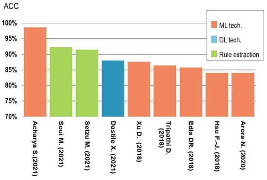
Figure 12.
Comparison of accuracy of various methods for the German (categorical) dataset [27,40,42,44,46,51,54,82,83].
Numerous studies have investigated accuracy and interpretability pairs (defined in this paper as a reciprocal of the number of rules); thus, a tradeoff curve between accuracy and interpretability based on recent reports on the German (categorical) dataset and Figure 7 in the study by Gunnarsson et al. [9] is shown in Figure 13. As shown in the figure, after conducting appropriate preprocessing and feature selection of input variables for specific datasets, the accuracy (92.3%) and interpretability (5.1 rules) are beyond the tradeoff curve (in blue) and close to the ideal point (upper right corner in red). (See Table 15). Thus, the so-called accuracy–interpretability dilemma is apparently relaxed. The highest accuracy obtained by all DL-based and ML classifiers is plotted along the Y-axis; no interpretability exhibits an infinite number of rules. The green dot shows the highest classification accuracy. This can be interpreted as the existence of an infinite number of rules, which means zero (0) interpretability.
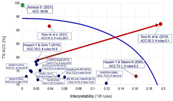
Figure 13.
Tradeoff curve between accuracy and interpretability for the German (categorical) dataset [1,31,40,82,83,88].
Table 15.
Performance of ensemble and hybrid classifiers, rule-based classifiers, and deep-learning-based classifiers for the German (categorical) dataset.
6.3.3. Accuracy of Deep-Learning-Based Classifiers in Credit Scoring for the German (Numerical) Dataset
Figure 14 shows that two DL-based classifiers are amongst the top five models with the highest accuracy for the German (numerical) dataset. Notably, the sixth-highest classifier is a hybrid of CNN and XGBoost [64]. The German (numerical) dataset is composed of 24 numerical attributes. The DL cascade ensemble system in DGHNL achieved an accuracy of 94.6%.
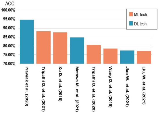
Figure 14.
Comparison of accuracy of various methods for the German (numerical) dataset [23,25,48,51,58,59,61,64].
6.3.4. Accuracy for Deep-Learning-Based Classifiers in Credit Scoring for Japanese Dataset
Figure 15 shows that one DL technique classifier and one rule extraction method are amongst the top five methods with the highest accuracies on the Japanese dataset. The DL classifier consisting of the hybrid discriminant model and DF proposed by Li et al. [50] achieved the second-highest accuracy of 89.86%, which is relatively close to the highest accuracy obtained by the ensemble and hybrid classifier proposed by Zhang et al. [47].
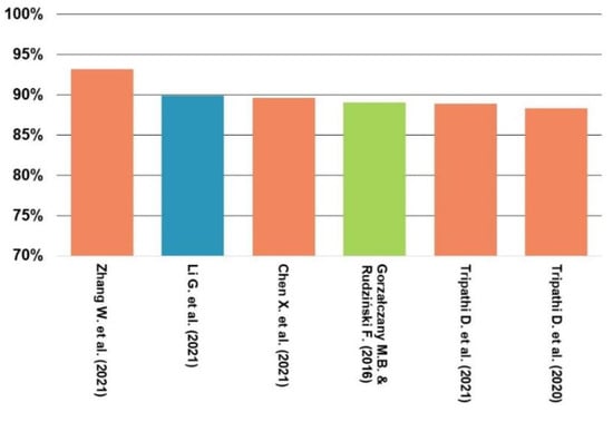
Figure 15.
Comparison of accuracy of various methods for the Japanese dataset [47,48,50,58,62,91].
6.3.5. Accuracy of Deep-Learning-Based Classifiers in Credit Scoring for the Taiwanese Dataset
Figure 16 shows that the DL classifier proposed by Li et al. [50] achieved the highest accuracy (89.86%) for the Taiwanese dataset, followed by that proposed by Tripathi [58] (89.44%). Li et al. also proposed a novel two-stage hybrid model by combining multiple feature selection methods and gcForest [35,36]. In this model, the differences and complementarities between conventional statistical and artificial intelligence (AI) models were considered. Although gcForest performs well in many fields, it is yet to be applied to credit scoring, even though it has exhibited better predictive performance and robustness [47].
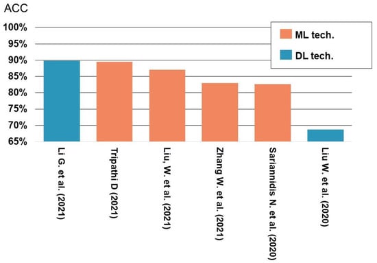
Figure 16.
Comparison of accuracy of various classifiers for the Taiwanese dataset [47,50,58,61,63].
6.4. Classifier Design Using Convolutional Neural Networks (CNNs) for Credit Scoring Datasets
Although the DNN architecture of a deep cascade ensemble classifier differs from that of a CNN, deep cascade layers can be designed as shown in Figure 8 [24]. As described previously, a CNN is not suitable for constructing high-performance classifiers. However, Pławiak et al. [24] first inspired this deep cascade ensemble architecture for a unique classifier system and proposed DGHNL [23]. A similar approach using a DBN proposed by Metawa et al. [25] revealed promising accuracy for the Australian dataset.
Gunnarsson et al. [9] concluded that DBNs do not outperform shallower networks with one hidden layer. The data structure for the implementation of a DBN is 1D, whereas that for the implementation of a CNN is 2D. Thus, comparisons of deep networks with several hidden layers (i.e., DBNs) and shallower networks with one hidden layer are simple. By contrast, comparisons of ensemble and hybrid classifiers with and without DL techniques are theoretically and structurally difficult.
If interpretability of the model’s prediction is critical, SMOPSO would be the first choice shown in Figure 13. Although DL techniques are not fully used CNN structures, certain DL-based classifiers appear amongst the top five methods with the highest accuracy. The performances realised are higher than expected. Generally, CNNs largely benefit from their feature-learning power to determine meaningful features captured in the 2D data structure. Generally, CNNs can achieve reasonable performance with default hyperparameter settings; however, extensive hyperparameter tuning is typically required to achieve the best performance. Thus, for highly imbalanced datasets with many nominal attributes, the predictive model generated by the CNN may pose formidable challenges [92].
6.5. Re-Evaluation of Rule Extraction and Rule-Based Methods for Explainable Machine Learning (ML) in Credit Scoring
Rudin suggested the complete avoidance of “black box” ML, as DL should be able to explain the obtained classification results by itself [93]. Rudin also showed that simple models such as linear regression and rule-based learners achieved performance that is comparable to complicated models such as DL models, ensemble models, and RF. Moreover, there exists no noticeable difference in their performance. Dastile and Celik [27] proposed unique methods for explainable DL classifiers and compared their performance with prediction models using Grad-CAM [94], LIME [95], SHAP values [96], and saliency maps [97]. These explanation methods all highlight important regions/pixels corresponding to the output/prediction class in an image.
However, since most of these tools require additional feature engineering and cannot always explain the reasoning behind a decision, they can still be used to complement LIME and other tools [98]. In addition, all these models follow the model-agnostic approach as opposed to the model-specific interpretability method because the latter is associated with lower accuracy and the use of a single algorithm. By contrast, the model-agnostic approach extracts explanations by treating the model as a “black box” while ruffling the model inputs and examining how it reacts, as opposed to inspecting the internal model parameters.
On the contrary, the author believes that rules are one of the most popular symbolic representations of knowledge discovered from data [99] and are more comprehensible, particularly “black boxes” such as the regions/pixels in an image, than are other representations. In fact, Dastile and Celik [27] also noted that they should focus on validating and evaluating performance by using domain experts in the field of credit scoring, such as credit risk analysts or managers. In such a case, rules become much more explainable and qualitatively analytical. Therefore, attempts should be made to bridge regions/pixels in an image and the symbolic rules for credit scoring in business analytics. The findings of the present review strongly suggest the considerable potential of explainable DL-based classifiers.
Very recently, Gamona et al. (2022) [100] reported a sensational study on black boxes, which fills a literature gap by showing how it is possible to fit a very precise ML model that is highly interpretable by using XGBoost and applying new model interpretability improvements. Although XGBoost is the de facto standard in data science community and a formidable competitor to DL models, the authors substantially criticise the interpretability of XGBoost. Xia et al. (2022) [101] proposed a heterogeneous deep forest model that combines a DL architecture and tree-based ensemble classifiers as the modelling approach. They proposed a heterogeneous deep forest (HDF) method and its variants, combining DLcombine and GBDT-based methods [102], which significantly outperform the industry benchmarks, logistic regression and RF, as well as DNN and DBN, across multiple datasets and evaluation measures. They concluded that DL algorithms have the potential of building effective credit scoring models depending on the architecture. References [100,101] are published in finance journals rather than computer science journals. There are many approaches to explain the form of rules for complex trees and deep learning models.
6.6. Rule Extraction from Images Using a Convolutional Neural Network (CNN)
As described in Section 4, credit scoring methods based on 2D CNN and rule extraction from images using CNN are closely related to the topic of this review. Angelov and Soares [103] proposed the novel xDNN approach to achieve a moderate level of explainability combined with high accuracy. xDNN is based on a novel DL architecture that combines reasoning and learning synergistically. The noniterative and nonparametric architecture is efficient in terms of time and computational resources. Moreover, the approach can be understood by humans and outperforms well-known image-processing methods and DL methods in terms of accuracy and training time. In addition, it includes an explainable classifier.
For high-dimensional input data such as images, the individual pixels are not easily interpretable. Therefore, rule extraction and rule-based approaches are not typically used for such high-dimensional data. However, Burkhardt et al. [104] introduced first-order convolutional rules, which are logical rules that can be extracted using a CNN; their complexity depends on the size of the convolutional filter and not on the dimension of the input. They demonstrated the potential of rule-based approaches for three well-known images by combining the advantages of NNs and rule learning.
On the contrary, D’Alberto et al. (2022) [105] presented xDNN, an end-to-end system for DL inference based on a family of specialised hardware processors synthesised on field-programmable gate arrays (FPGAs) and CNNs. They presented a design optimised for low latency, high throughput, and high computing efficiency with no batching. This paper did not contain a proof-of-concept; however, because the authors work at Xilinxan innovative semiconductor company that primarily supplies programmable logic devices and has been recently acquired by AMD., it is reasonable to believe that this type of hardware can be easily realised at low cost using FPGA.
6.7. Limitations of this Work
The credit scoring models in this study mostly require offline training using credit scoring datasets. In the future, online training using a larger number of credit scoring datasets will be conducted.
7. Promising Research Directions
Post the 2021 emergence of DL-based classifiers with high accuracies for credit scoring, the author believes that two promising research directions exist, as explained below.
The first is the use of a DL-inspired ensemble system [24,34]. The key aspect of a DL-inspired ensemble system is the inclusion of ML elements that are distributed in cascade and/or parallel ensembles hierarchically. As shown in Section 6.2, DGCEC [23] and DGHNL [24], as typical DL-inspired ensemble systems, achieved very high accuracies for credit scoring datasets consisting of only numerical attributes, such as the Australian, German (numerical), and Japanese datasets. A hybrid ensemble classifier with DBN [20] and deep forest [36,37] also achieved very high accuracies for the Japanese and Taiwanese datasets.
The credit scoring models and their applications in peer-to-peer (P2P) lending (which consists of individual lenders who provide loans to individual borrowers on an electronic platform) are still immature owing to the different characteristics of P2P lending [106]. Chen et al. [107] proposed a credit assessment model for banks to assess the risk of default for home credit based on DeepGBM [108]; however, their model did not consider deviations caused by changes in the distribution of the data and cannot be updated online. Although substantial progress has been made, no similar attempts have been made for credit scoring in P2P lending. However, a deep sequential model ensemble [109] has been proposed for the detection of credit card fraud.
Research on DL-based credit scoring has begun only recently and has the potential to significantly impact the working of banks and other financial intuitions. However, increases in the volume and velocity of credit card transactions can cause class imbalance and concept deviation problems in datasets where credit card fraud is detected, which may make it very difficult for traditional approaches to produce robust detection models. To address this, Sinanc et al. [110] proposed a novel approach called fraud detection with image conversion.
In the general CNN structure, high-dimensional input data, such as images, are not easily interpretable. Although DL techniques are not fully used CNN structures, certain DL-based classifiers in this review ranked amongst the top five classifiers with the highest accuracy. The performances currently being achieved are higher than expected.
Currently, most existing credit scoring models are implemented with shallow structures; thus, DL is innovatively introduced into the credit scoring model; for example, the use of XGBoost for credit scoring [67]. Jiao et al. [67] proposed a unique bidirectional optimization structure that simultaneously optimises both CNN and XGBoost by using APSO. Optimizing a CNN to extract deep features is more suitable for XGBoost and optimizing XGBoost makes the model structure match the extracted features, which provides a better understanding of the image features. Bidirectional optimization maintains the characteristics of both parts while allowing them to be combined more closely together and enabling the features of the fully extracted image to be used for classification. The classification accuracy reported by Jiao et al. [67] for the German (numerical) and Taiwanese datasets ranked very highly for these two datasets; thus, it is reasonable to believe that this simple idea of DL-based classifiers could help simultaneously deal with structured and unstructured datasets.
In 2022, Du and Shu [111] proposed a model that uses logistic regression), BRNN (bidirectional recurrent neural network), and XGBoost for credit scoring. The model achieved an AUC of 0.9574 and accuracy of 89.35% for the Australian dataset. The model also achieved an AUC of 0.8374 and accuracy of 77.5% for the German (categorical) dataset. In [112], a novel financial distress prediction model uses an adaptive whale optimization algorithm with a deep learning (AWOA-DL) technique, including a multi-layer perceptron (MLP) and optimization algorithm. In the experiments, the AWOA-DL algorithm showed the best performance with maximum accuracy of 0.9689 for the Australian dataset.
The second research direction is to develop a class-imbalanced XGBoost as well as multiclass classification, which are of great practical significance in the field of business analytics and can be applied in the areas of credit scoring, credit card fraud detection, bankruptcy and digital marketing. However, considering the nature of data structure, such datasets are not only imbalanced but also contain many nominal attributes, making it technically difficult to achieve high classification accuracy. Undoubtedly, DL- based classifiers also constitute an urgent research issue as well and many techniques have been discussed in this review that can classify structured data with high accuracy.
The third research direction is to convert tabular datasets into images using bins employed to calculate WOE. Each pixel of a feature image corresponds to a feature bin. WOE is used to create meaningful bins that are monotonic to the response variable. Dastile and Celik [27] considered both continuous and categorical features, and their proposed method achieved the highest accuracy (88%) amongst the DL-based classifiers for the German (categorical) dataset. In 2022, Borisov et al. [113] proposed the DeepTLF (https://github.com/unnir/DeepTLF, accessed on 1 January 2022) framework for deep tabular learning. The core idea of their method is to transform the heterogeneous input data into homogeneous data to boost the performance of DNNs considerably.
In contrast to a previous study [76], they systematically discretised tabular data into optimal categories by using WOE and utilised both categorical and continuous features. Considering the practical applications of business analytics for credit scoring, such conversions are required to deal with both numerical and categorical datasets. As credit scoring datasets are stored in the databases of banks and the other financial institutions, they can be used for P2P lending [106].
However, the use of credit scoring models in P2P lending involves certain limitations. First, the feature space of P2P credit data usually contains two types of features: dense numerical features (e.g., amount of the loan, asset-to-liability ratio) and sparse categorical features (e.g., gender, credit score). However, existing classifiers, including DT classifiers and NN models, are typically useful for processing only one data type. Zhang et al. [106] previously developed an effective model with multiple data types for P2P lending credit datasets. Therefore, developing an accurate and efficient method for converting tabular data into categorical and continuous features is a promising direction for future studies. The accuracy of these approaches should be enhanced, and suitable methods should be investigated to improve interpretability in banks and other financial intuitions.
Finally, a tree diagram of topics for future development is provided here. As very early works, all papers with reference numbers are scattered in Figure 17. These papers are pioneering works and more advanced technologies will be developed in the near future.
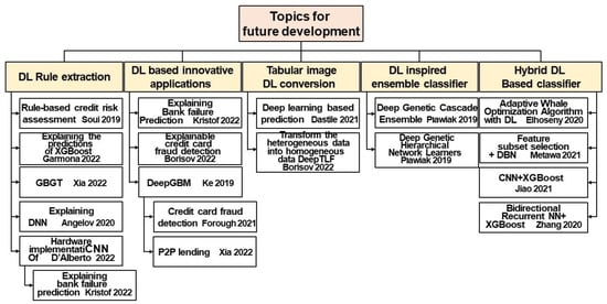
Figure 17.
Tree diagram of topics for future development [23,25,27,56,64,83,100,101,103,105,108,109,112,113,114].
8. Concluding Remarks and Future Scope of Work
Based on the above discussion, it can be concluded that there is a need to actively aim towards not only high quantitative performance, such as in predictive accuracy, but also high qualitative performance, such as in interpretability shown in Figure 13. In response to social demands such as General Data Protection Regulations [115], xDNN was developed as an innovative approach that showed very high classification accuracy using images; however, its level of explainability was still quite low. As previously discussed, xDNN offers a novel DL architecture that synergistically combines reasoning and learning and has outperformed well-known image classification methods in terms of accuracy. Currently, xDNN algorithms are not easily adaptable to credit scoring because Angelov and Soares [103] simply prioritised the highest accuracy using complicated if–then rules, with the if part consisting of considerably large images. On the contrary, various tools have been developed for converting tabular data into images and a bidirectional optimization structure using both CNN and XGBoost.
Based on Section 6.4, Section 6.5, Section 6.6 and Section 7, it is reasonable to believe that many researchers may assume that there is no significant difference in classification accuracy no matter what method is used; however, this is true only when the degree of mission-criticality is not severe; exceptions include data in finance and medicine. Therefore, using XGBoost for structured data and DL for classification of unstructured data (i.e., images) is simple and quite traditional. In addition, if there is no significant difference in accuracy, improving interpretability is an invaluable option for wider adoption in various areas. A very recent study in finance, similar to the credit scoring framework, has been proposed that extracted rules to classify bank failure [114]. Research in the area of credit scoring or credit risk can contribute to the modernisation of financial engineering by simply introducing a time series so that the elemental technologies described in this review can be applied to financial distress, bankruptcy, peer-to-peer (P2P) lending, credit card fraud detection, and inclusion of macro-economic variables. Their findings are useful for bank supervisor authorities, bank executives, risk management professionals, as well as policymakers in the field of finance.
At present, we are moving towards the intersection of the above research avenues to deal with both structured and unstructured data. DL would achieve not only very high accuracy for images but also high performance for structured data in explainable credit scoring. In a future work, an attempt will be made to bridge images and symbolic rules to realise AI finance.
Funding
This research received no external funding.
Data Availability Statement
UCI Machine Learning Repository https://archive.ics.uci.edu/ml/index.php; GitHub german-credit-data https://github.com/rajarshighoshal/german-credit-data/blob/master/README.md, accessed on 10 January 2020).
Acknowledgments
I would like to thank all graduate students for their continuous and faithful support.
Conflicts of Interest
The author declares that they have no known competing financial interests or personal relationships that could have appeared to influence the work reported in this paper.
References
- Hayashi, Y. Application of a rule extraction algorithm family based on the Re-RX algorithm to financial credit risk assessment from a Pareto optimal perspective. Oper. Res. Perspect. 2016, 3, 32–42. [Google Scholar] [CrossRef]
- Serrano-Cinca, C.; Gutiérrez-Nieto, B. The use of profit scoring as an alternative to credit scoring systems in peer-to-peer (P2P) lending. Decis. Support Syst. 2016, 89, 113–122. [Google Scholar] [CrossRef]
- Quinlan, J.R. Programs for Machine Learning; Morgan Kaufmann: San Mateo, Canada, 1993. [Google Scholar]
- Setiono, R.; Baesens, B.; Mues, C. Recursive neural network rule extraction for data with mixed attributes. IEEE Trans. Neural Netw. 2008, 19, 299–307. [Google Scholar] [CrossRef] [PubMed]
- Martens, D.; Baesens, B.; Van Gestel, T.; Vanthienen, J. Comprehensible credit scoring models using support vector machines. Eur. J. Oper. Res. 2007, 183, 1488–1497. [Google Scholar] [CrossRef]
- Breiman, L. Bagging predictors. Mach. Learn. 1996, 24, 123–140. [Google Scholar] [CrossRef]
- Freund, Y.; Schapire, R.E. A decision-theoretic generalization of online earning and an application to boosting. J. Comput. Syst. Sci. 1997, 55, 119–139. [Google Scholar] [CrossRef]
- Kraus, M.; Feuerriegel, S.; Oztekin, A. Deep learning in business analytics and operations research: Models, applications and managerial implications. Eur. J. Oper. Res. 2020, 281, 628–641. [Google Scholar] [CrossRef]
- Gunnarsson, B.R.; vanden Broucke, S.; Baesens, B.; Óskarsdóttir, M.; Lemahieu, W. Deep learning for credit scoring: Do or don’t? Eur. J. Oper. Res. 2021, 295, 292–305. [Google Scholar] [CrossRef]
- Chen, T.; Guestrin, C. XGBoost: A scalable tree boosting system. In Proceedings of the 22nd ACM SIG KDD International Conference on Knowledge Discovery and Data Mining, ACM, San Francisco, CA, USA, 13 August 2016; pp. 785–794. [Google Scholar]
- Cun, Y.L.; Boser, B.; Denker, J.S.; Henderson, D.; Howard, R.E.; Hubbard, W.; Jackel, L.D. Handwritten digit recognition with a back-propagation network. In Proceedings of the Advances in Neural Information Processing Systems, Denver, CO, USA, 26–29 November 1990; pp. 396–404. [Google Scholar]
- Hochreiter, S.; Schmidhuber, J. Long short-term memory. Neural Comput. 1997, 9, 1735–1780. [Google Scholar] [CrossRef]
- Han, H.; Li, Y.; Zhu, X. Convolutional neural network learning for generic data classification. Inf. Sci. 2019, 477, 448–465. [Google Scholar] [CrossRef]
- Sezer, O.B.; Gudelek, M.U.; Ozbayoglu, A.M. Financial time series forecasting with deep learning: A systematic literature review: 2005–2019. Appl. Soft Comput. J. 2020, 90, 106181. [Google Scholar] [CrossRef]
- Dastile, X.; Celik, T.; Potsane, M. Statistical and machine learning models in credit scoring: A systematic literature survey. Appl. Soft Comput. 2020, 91, 106263. [Google Scholar] [CrossRef]
- Luo, C.; Wu, D.; Wu, D. A deep learning approach for credit scoring using credit default swaps. Eng. Appl. Artif. Intell. 2017, 65, 465–470. [Google Scholar] [CrossRef]
- Tran, K.; Duong, T.; Ho, Q. Credit scoring model: A combination of genetic programming and deep learning. In Proceedings of the 2016 Future Technology Conference, FTC, San Francisco, CA, USA, 6–7 December 2016; pp. 145–149. [Google Scholar]
- Ozbayoglu, A.M.; Gudelek, M.U.; Sezer, O.B. Deep learning for financial applications: A survey. Appl. Soft Comput. 2020, 93, 106384. [Google Scholar] [CrossRef]
- Yu, L.; Zhou, R.; Tang, L.; Chen, R. A DBN-based resampling SVM ensemble learning paradigm for credit classification with imbalanced data. Appl. Soft Comput. 2018, 69, 192–202. [Google Scholar] [CrossRef]
- Hinton, G.E.; Salakhutdinov, R.R. Reducing the dimensionality of data with neural networks. Science 2006, 313, 504–507. [Google Scholar] [CrossRef]
- Vincent, P.; Larochelle, H.; Bengio, Y.; Manzagol, P.A. Extracting and composing robust features with denoising autoencoders. In Proceedings of the 25th International Conference on Machine Learning, ACM, Helsinki, Finland, 5–9 July 2008; pp. 1096–1103. [Google Scholar]
- Tomczak, J.M.; Zięba, M. Classification restricted Boltzmann machine for comprehensible credit scoring model. Expert Syst. Appl. 2015, 42, 1789–1796. [Google Scholar] [CrossRef]
- Pławiak, P.; Abdar, M.; Rajendra Acharya, U.R. Application of new deep genetic cascade ensemble of SVM classifiers to predict the Australian credit scoring. Appl. Soft Comput. 2019, 84, 105740. [Google Scholar] [CrossRef]
- Pławiak, P.; Abdar, M.; Pławiak, J.; Makarenkov, V.; Rajendra Acharya, U.R. DGHNL: A new deep genetic hierarchical network of learners for prediction of credit scoring. Inf. Sci. 2020, 516, 401–418. [Google Scholar] [CrossRef]
- Metawa, N.; Pustokhina, I.V.; Pustokhin, D.A.; Shankar, K.; Elhoseny, M. Computational intelligence-based financial crisis prediction model using feature subset selection with optimal deep belief network. Big Data 2021, 9, 100–115. [Google Scholar] [CrossRef]
- Thomas, L.C.; Edelman, D.B.; Crook, J.N. Credit Scoring and Its Applications; Siam: Philadelphia, PA, USA, 2002. [Google Scholar]
- Dastile, X.; Celik, T. Making deep learning-based predictions for credit scoring explainable. IEEE Access 2021, 9, 50426–50440. [Google Scholar] [CrossRef]
- Freund, Y.; Haussler, D. Unsupervised learning of distributions of binary vectors using 2-layer networks. In Advances in Neural Information Processing Systems 4; Moody, J., Hanson, S.J., Lippmann, R., Eds.; Morgan Kaufmann: San Francisco, CA, USA, 1991; pp. 912–919. [Google Scholar]
- LeCun, Y.; Bengio, Y.; Hinton, G. Deep learning. Nature 2015, 521, 436–444. [Google Scholar] [CrossRef] [PubMed]
- Bologna, G.; Hayashi, Y. A comparison study on rule extraction from neural network ensembles, boosted shallow trees, and SVMs. Appl. Comp. Intell. Soft Comput. 2018, 2018, 4084850. [Google Scholar] [CrossRef]
- Hayashi, Y.; Takano, N. One-dimensional convolutional neural networks with feature selection for highly concise rule extraction from credit scoring datasets with heterogeneous attributes. Electronics 2020, 9, 1318. [Google Scholar] [CrossRef]
- Liu, K.; Kang, G.; Zhang, N.; Hou, B. Breast cancer classification based on fully-connected layer first convolutional neural networks. IEEE Access 2018, 6, 23722–23732. [Google Scholar] [CrossRef]
- Hayashi, Y.; Tanaka, Y.; Takagi, T.; Saito, T.; Iiduka, H.; Kikuchi, H.; Bologna, G.; Mitra, S. Recursive-rule extraction algorithm with J48graft and applications to generating credit scores. J. Artif. Intell. Soft Comput. Res. 2016, 6, 35–44. [Google Scholar] [CrossRef]
- Szegedy, C.; Liu, W.; Jia, Y.; Sermanet, P.; Reed, S.; Anguelov, D.; Erhan, D.; Vanhoucke, V.; Rabinovich, A. Going deeper with convolutions. In Proceedings of the 2015 IEEE Conference on Computer Vision and Pattern Recognition (CVPR), Boston, MA, USA; 2015; pp. 1–9. [Google Scholar]
- Zhou, Z.H.; Feng, J. Deep forest: Towards an alternative to deep neural networks. In Proceedings of the 26th International Joint Conference on Artificial Intelligence, Melbourne, Australia, 19–25 August 2017; pp. 3553–3559. [Google Scholar]
- Zhou, Z.H.; Feng, J. Deep forest. Natl. Sci. Rev. 2019, 6, 74–86. [Google Scholar] [CrossRef]
- Liang, Q.; Wang, K. Distributed outlier detection in hierarchically structured datasets with mixed attributes. Qual. Technol. Quant. Manag. 2020, 17, 337–353. [Google Scholar] [CrossRef]
- Domingo-Ferrer, J.; Solanas, A. A measure of variance for hierarchical nominal attributes. Inf. Sci. 2008, 178, 4644–4655. [Google Scholar] [CrossRef]
- Zhang, Y.; Cheung, Y.M.; Tan, K.C.A. Unified, a unified entropy-based distance metric for ordinal-and-nominal-attribute data clustering. IEEE Trans. Neural Netw. Learn. Syst. 2020, 31, 39–52. [Google Scholar] [CrossRef]
- Acharya, S.; Pustokhina, I.V.; Pustokhin, D.A.; Geetha, B.T.; Joshi, G.P.; Nebhen, J.; Yang, E.; Seo, C. An improved gradient boosting tree algorithm for financial risk management. Knowl. Manag. Res. Pract. 2021, 1–12. [Google Scholar] [CrossRef]
- Kuppili, V.; Tripathi, D.; Reddy Edla, D.R. Credit score classification using spiking extreme learning machine. Comp. Intell. 2020, 36, 402–426. [Google Scholar] [CrossRef]
- Tripathi, D.; Edla, D.R.; Cheruku, R. Hybrid credit scoring model using neighborhood rough set and multi-layer ensemble classification. J. Intell. Fuzzy Syst. 2018, 34, 1543–1549. [Google Scholar] [CrossRef]
- Radović, O.; Marinković, S.; Radojičić, J. Credit scoring with an ensemble deep learning classification methods—Comparison with traditional methods. Facta Univ. Ser. Econ. Organ. 2021, 18, 29–43. [Google Scholar] [CrossRef]
- Hsu, F.J.; Chen, M.Y.; Chen, Y.C. The human-like intelligence with bio-inspired computing approach for credit ratings prediction. Neurocomputing 2018, 279, 11–18. [Google Scholar] [CrossRef]
- Tripathi, D.; Edla, D.R.; Cheruku, R.; Kuppili, V. A novel hybrid credit scoring model based on ensemble feature selection and multilayer ensemble classification. Comp. Intell. 2019, 35, 371–394. [Google Scholar] [CrossRef]
- Edla, D.R.; Tripathi, D.; Cheruku, R.; Kuppili, V. An efficient multi-layer ensemble framework with BPSOGSA-based feature selection for credit scoring data analysis. Arab. J. Sci. Eng. 2018, 43, 6909–6928. [Google Scholar] [CrossRef]
- Zhang, W.; Yang, D.; Zhang, S.; Ablanedo-Rosas, J.H.; Wu, X.; Lou, Y. A novel multi-stage ensemble model with enhanced outlier adaptation for credit scoring. Expert Syst. Appl. 2021, 165, 113872. [Google Scholar] [CrossRef]
- Tripathi, D.; Edla, D.R.; Kuppili, V.; Bablani, A. Evolutionary extreme learning machine with novel activation function for credit scoring. Eng. Appl. Artif. Intell. 2020, 96, 103980. [Google Scholar] [CrossRef]
- Xu, D.; Zhang, X.; Hu, J.; Chen, J. A novel ensemble credit scoring model based on extreme learning machine and generalized fuzzy soft sets. Math. Probl. Eng. 2020, 2020, 7504764. [Google Scholar] [CrossRef]
- Li, G.; Ma, H.D.; Liu, R.Y.; Shen, M.D.; Zhang, K.X. A two-stage hybrid default discriminant model based on Deep Forest. Entropy 2021, 23, 582. [Google Scholar] [CrossRef] [PubMed]
- Xu, D.; Zhang, X.; Feng, H. Generalized fuzzy soft sets theory-based novel hybrid ensemble credit scoring model. Int. J. Fin. Econ. 2019, 24, 903–921. [Google Scholar] [CrossRef]
- Zhang, H.; He, H.; Zhang, W. Classifier selection and clustering with fuzzy assignment in ensemble model for credit scoring. Neurocomputing 2018, 316, 210–221. [Google Scholar] [CrossRef]
- Trivedi, S.K. A study on credit scoring modeling with different feature selection and machine learning approaches. Technol. Soc. 2020, 63, 101413. [Google Scholar] [CrossRef]
- Arora, N.; Kaur, P.D. A Bolasso based consistent feature selection enabled random forest classification algorithm: An application to credit risk assessment. Appl. Soft Comput. 2020, 86, 105936. [Google Scholar] [CrossRef]
- Yu, L.; Wang, S.; Lai, K.K. An intelligent-agent-based fuzzy group decision making model for financial multi criteria decision support: The case of credit scoring. Eur. J. Oper. Res. 2009, 195, 942–959. [Google Scholar] [CrossRef]
- Zhang, T.; Chi, G. A heterogeneous ensemble credit scoring model based on adaptive classifier selection: An application on imbalanced data. Int. J. Fin. Econ. 2020, 26, 4372–4385. [Google Scholar] [CrossRef]
- Song, Y.; Peng, Y. A MCDM-based evaluation approach for imbalanced classification methods in financial risk prediction. IEEE Access 2019, 7, 84897–84906. [Google Scholar] [CrossRef]
- Tripathi, D.; Edla, D.R.; Bablani, A.; Shukla, A.K.; Reddy, B.R. Experimental analysis of machine learning methods for credit score classification. Prog. Artif. Intell. 2021, 10, 217–243. [Google Scholar] [CrossRef]
- Wang, D.; Zhang, Z.; Bai, R.; Mao, Y. A hybrid system with filter approach and multiple population genetic algorithm for feature selection in credit scoring. J. Comp. Appl. Math. 2018, 329, 307–321. [Google Scholar] [CrossRef]
- Lappas, P.Z.; Yannacopoulos, A.N. A machine learning approach combining expert knowledge with genetic algorithms in feature selection for credit risk assessment. Appl. Soft Comput. 2021, 107, 107391. [Google Scholar] [CrossRef]
- Liu, W.; Fan, H.; Xia, M. Multi-grained and multi-layered gradient boosting decision tree for credit scoring. Appl. Intell. 2022, 52, 5325–5341. [Google Scholar] [CrossRef]
- Chen, X.; Li, S.; Xu, X.; Meng, F.; Cao, W. A novel GSCI-based ensemble approach for credit scoring. IEEE Access 2020, 8, 222449–222465. [Google Scholar] [CrossRef]
- Sariannidis, N.; Papadakis, S.; Garefalakis, A.; Lemonakis, C.; Kyriaki-Argyro, T. Default avoidance on credit card portfolios using accounting, demographical and exploratory factors: Decision making based on machine learning (ML) techniques. Ann. Oper. Res. 2020, 294, 715–739. [Google Scholar] [CrossRef]
- Jiao, W.; Hao, X.; Qin, C. The image classification method with CNN-XGBoost model based on adaptive particle swarm optimization. Information 2021, 12, 156. [Google Scholar] [CrossRef]
- Shen, F.; Zhao, X.; Kou, G.; Alsaadi, F.E. A new deep learning ensemble credit risk evaluation model with an improved synthetic minority oversampling technique. Appl. Soft Comput. J. 2021, 98, 106852. [Google Scholar] [CrossRef]
- Han, H.; Wang, W.Y.; Mao, B.H. Borderline-SMOTE: A new over-sampling method in imbalanced data sets learning. Adv. Intell. Comput. 2005, 3644, 878–887. [Google Scholar] [CrossRef]
- Rätsch, G.; Onoda, T.; Müller, K.R. Soft margins for AdaBoost. Mach. Learn. 2001, 42, 287–320. [Google Scholar] [CrossRef]
- Eberhart, R.; Kennedy, J. A new optimizer using particle swarm theory. In Proceedings of the MHS’95, Sixth International Symposium on Micro Machine and Human Science, Nagoya, Japan, 4–6 October 1995; pp. 39–43. [Google Scholar]
- Neagoe, V.; Ciotec, A.; Cucu, G. Deep convolutional neural networks versus multilayer perceptron for financial prediction. In Proceedings of the 2018 International Conference on Communications (COMM), Bucharest, Romania, 14–16 June 2018; pp. 201–206. [Google Scholar]
- Hamori, S.; Kawai, M.; Kume, T.; Murakami, Y.; Watanabe, C. Ensemble learning or deep learning? Application to default risk analysis. J. Risk Financ. Manag. 2018, 11, 12. [Google Scholar] [CrossRef]
- Zhu, B.; Yang, W.; Wang, H.; Yuan, Y. A hybrid deep learning model for consumer credit scoring. In Proceedings of the International Conference on Artificial Intelligence and Big Data (ICAIBD), Chengdu, China, 26–28 May 2018; pp. 205–208. [Google Scholar]
- Breiman, L. Random forest. Mach. Learn. 2001, 45, 5–32. [Google Scholar] [CrossRef]
- Sun, B.; Yang, L.; Zhang, W.; Lin, M.; Dong, P.; Young, C.; Dong, J. SuperTML: Two-dimensional word embedding for the precognition on structured tabular data. arXiv 2019, arXiv:1903.06246. [Google Scholar]
- Han, H.; Zhu, X.; Li, Y. EDLT: Enabling deep learning for generic data classification. In Proceedings of the IEEE International Conference on Data Mining (ICDM), Singapore, 17–20 November 2018; IEEE: Washington, DC, USA, 2018. [Google Scholar] [CrossRef]
- Buturović, L.; Miljković, D. A novel method for classification of tabular data using convolutional neural networks. BioRxiv 2020. [Google Scholar] [CrossRef]
- Zhu, Y.; Brettin, T.; Xia, F.; Partin, A.; Shukla, M.; Yoo, H.; Evrard, Y.A.; Doroshow, J.H.; Stevens, R.L. Converting tabular data into images for deep learning with convolutional neural networks. Sci. Rep. 2021, 11, 11325. [Google Scholar] [CrossRef] [PubMed]
- Sharma, A.; Kumar, D. Non-image data Classification with convolutional neural networks. arXiv 2020, arXiv:2007.03218v1. [Google Scholar]
- He, C.; Ma, M.; Wang, P. Extract interpretability-accuracy balanced rules from artificial neural networks: A review. Neurocomputing 2020, 387, 346–358. [Google Scholar] [CrossRef]
- Dong, L.A.; Ye, X.; Yang, G. Two-stage rule extraction method based on tree ensemble model for interpretable loan evaluation. Inf. Sci. 2021, 573, 46–64. [Google Scholar] [CrossRef]
- Liang, Y.; Li, S.; Yan, C.; Li, M.; Jiang, C. Explaining the black-box model: A survey of local interpretation methods for deep neural networks. Neurocomputing 2021, 419, 168–182. [Google Scholar] [CrossRef]
- Lundberg, S.M.; Erion, G.; Chen, H.; DeGrave, A.; Prutkin, J.M.; Nair, B.; Katz, R.; Himmelfarb, J.; Bansal, N.; Lee, S.I. From local explanations to global understanding with explainable AI for trees. Nat. Mach. Intell. 2020, 2, 56–67. [Google Scholar] [CrossRef]
- Setzu, M.; Guidotti, R.; Monreale, A.; Turini, F.; Pedreschi, D.; Giannotti, F. GlocalX—From local to global explanations of black box AI models. Artif. Intell. 2021, 294, 103457. [Google Scholar] [CrossRef]
- Soui, M.; Gasmi, I.; Smiti, S.; Ghédira, K. Rule-based credit risk assessment model using multi-objective evolutionary algorithms. Expert Syst. Appl. 2019, 126, 144–157. [Google Scholar] [CrossRef]
- Wolpert, D.H. The existence of a priori distinctions between learning algorithms. Neural Comput. 1996, 8, 1391–1420. [Google Scholar] [CrossRef]
- Wolpert, D.H. The lack of a priori distinctions between learning algorithms. Neural Comput. 1996, 8, 1341–1390. [Google Scholar] [CrossRef]
- Giri, P.K.; De, S.S.; Dehuri, S.; Cho, S.B. Biogeography based optimization for mining rules to assess credit risk. Intell. Syst. Acc. Fin. Manag. 2021, 8, 35–51. [Google Scholar] [CrossRef]
- Gómez, D.; Rojas, A. An empirical overview of the no-free-lunch theorem and its effect on real-world machine learning classification. Neural Comput. 2016, 28, 216–228. [Google Scholar] [CrossRef] [PubMed]
- Hayashi, Y. Use of a deep belief network for small high-level abstraction data sets using artificial intelligence with rule extraction. Neural Comput. 2018, 30, 3309–3326. [Google Scholar] [CrossRef]
- Le Roux, N.L.; Bengio, Y. Representational power of restricted Boltzmann machines and deep belief networks. Neural Comput. 2008, 20, 1631–1649. [Google Scholar] [CrossRef]
- Hornik, K.; Stinchcombe, M.; White, H. Multilayer feedforward networks are universal approximators. Neural Netw. 1989, 2, 359–366. [Google Scholar] [CrossRef]
- Gorzałczany, M.B.; Rudziński, F. A multi-objective genetic optimization for fast, fuzzy rule-based credit classification with balanced accuracy and interpretability. Appl. Soft Comput. 2016, 40, 206–220. [Google Scholar] [CrossRef]
- Park, Y.; Ho, J.C. Tackling overfitting in boosting for noisy healthcare data. IEEE Trans. Knowl. Data Eng. 2022, 33, 2995–3006. [Google Scholar] [CrossRef]
- Rudin, C. Stop explaining black box machine learning models for high stakes decisions and use interpretable models instead. Nature Mach. Intell. 2019, 1, 206–215. [Google Scholar] [CrossRef]
- Selvaraju, R.R.; Cogswell, M.; Das, A.; Vedantam, R.; Parikh, D.; Batra, D. Grad-CAM: Visual explanations from deep networks via gradient-based localization. In Proceedings of the IEEE International Conference on Computer Vision (ICCV), Venice, Italy, 22–29 October 2017; pp. 618–626. [Google Scholar]
- Ribeiro, M.T.; Singh, S.; Guestrin, C. “Why should I trust you?” Explaining the predictions of any classifier. In Proceedings of the CoRR, San Francisco, CA, USA, 13–17 August 2016; pp. 1135–1144. [Google Scholar]
- Lundberg, S.; Lee, S.I. A unified approach to interpreting model predictions. arXiv 2017, arXiv:1705.07874. [Google Scholar]
- Samek, W.; Montavon, G.; Vedaldi, A.; Hansen, L.K.; Müller, K.R. (Eds.) Explainable AI: Interpreting, Explaining and Visualizing Deep Learning; Springer: Cham, Switzerland, 2019; Available online: https://link.springer.com/book/10.1007/978-3-030-28954-6 (accessed on 1 July 2022).
- Akinosho, T.D.; Oyedele, L.O.; Bilal, M.; Ajay, A.O.; Delgado, M.D.; Akinade, O.O.; Ahmed, A.A. Deep learning in the construction industry: A review of present status and future innovations. J. Build. Eng. 2020, 32, 101827. [Google Scholar] [CrossRef]
- Napierala, K.; Stefanowski, J. BRACID: A comprehensive approach to learning rules from imbalanced data. J. Intell. Inf. Syst. 2012, 39, 335–373. [Google Scholar] [CrossRef]
- Garmona, P.; Dwekat, A.; Mardawi, Z. No more black boxes! Explaining the predictions of a machine learning XGBoost classifier algorithm in business failure. Res. Int. Bus. Fin. 2022, 61, 101649. [Google Scholar] [CrossRef]
- Xia, Y.; Guo, X.; Li, Y.; He, L.; Chen, X. Deep learning meets decision trees: An application of a heterogeneous deep forest approach in credit scoring for online consumer lending. J. Forecast. 2022, 1–22. [Google Scholar] [CrossRef]
- Friedman, J.H. Greedy function approximation: A gradient boosting machine. Ann. Stat. 2001, 29, 1189–1232. [Google Scholar] [CrossRef]
- Angelov, P.; Soares, E. Towards explainable deep neural networks (xDNN). Neural Netw. 2020, 130, 185–194. [Google Scholar] [CrossRef]
- Burkhardt, S.; Brugger, J.; Wagner, N.; Ahmadi, Z.; Kersting, K.; Kramer, S. Rule extraction from binary neural networks with convolutional rules for model validation. Front. Artif. Intell. 2021, 4, 642263. [Google Scholar] [CrossRef]
- D’Alberto, P.; Wu, V.; Ng, A.; Nimaiyar, R.; Delaye., E. xDNN: Inference for deep convolutional neural networks.Deep Convolutional Neural Networks. ACM Trans. Reconfigurable Technol. Syst. 2022, 15, 1–29. [Google Scholar] [CrossRef]
- Zhang, Z.; Niu, K.; Liu, Y. A deep learning based online credit scoring model for P2P lending. IEEE Access 2020, 8, 177317. [Google Scholar] [CrossRef]
- Chen, X.; Liu, Z.; Zhong, M.; Liu, X.; Song, P. A deep learning approach using DeepGBM for credit assessment. In Proceedings of the Robotics, Intelligent Control and Artificial Intelligence (RICAI), Shanghai, China, 20–22 September 2019; pp. 774–779. [Google Scholar]
- Ke, G.; Xu, Z.; Zhang, J.; Bian, J.; Liu, T.Y. DeepGBM: A deep learning framework distilled by GBDT for online prediction tasks. In Proceedings of the 25th ACM SIGKDD International Conference on Knowledge Discovery Data Mining, Anchorage, AK, USA, 4–8 August 2019; pp. 384–394. [Google Scholar]
- Forough, J.; Momtazi, S. Ensemble of deep sequential models for credit card fraud detection. Appl. Soft Comput. 2021, 99, 106883. [Google Scholar] [CrossRef]
- Sinanc, D.; Demirezen, U.M.; Sağıroğlu, S. Explainable credit card fraud detection with image conversion. ADCAIJ 2021, 10, 63–76. [Google Scholar] [CrossRef]
- Du, P.; Shu, H. Exploration of financial market credit scoring and risk management and prediction using deep learning and bionic algorithm. J. Glob. Inform. Manag. 2022, 30, 1–29. [Google Scholar] [CrossRef]
- Elhoseny, M.; Metawa, N.; Sztano, G. Deep learning-based model for financial distress prediction. Ann. Oper. Res. 2020. [Google Scholar] [CrossRef] [PubMed]
- Borisov, V.; Broelemann, K.; Kasneci, E.; Gjergji Kasneci, G. DeepTLF: Robust deep neural networks for heterogeneous tabular data. Int. J. Data Sci. Anal. 2022. [Google Scholar] [CrossRef]
- Kristóf, T.; Virág., M. EU-27 bank failure prediction with C5.O decision trees and deep learning neural networks. Res. Int. Bus. Fin. 2022, 61, 101644. [Google Scholar] [CrossRef]
- European Parliament and Council. Regulation 2016/679 on the protection of natural persons with regard to the processing of personal data and on the free movement of such data, and repealing Directive 95/46/EC (General Data Protection Regulation). Off. J. Eur. Union 2016, 59, 1. [Google Scholar]
Publisher’s Note: MDPI stays neutral with regard to jurisdictional claims in published maps and institutional affiliations. |
© 2022 by the author. Licensee MDPI, Basel, Switzerland. This article is an open access article distributed under the terms and conditions of the Creative Commons Attribution (CC BY) license (https://creativecommons.org/licenses/by/4.0/).