Article

Feature Selection Techniques for Big Data Analytics

by
Waleed Albattah
1,
Rehan Ullah Khan
1,
Mohammed F. Alsharekh
2,* and
Samer F. Khasawneh
3
1
Department of Information Technology, College of Computer, Qassim University, Buraydah 52571, Saudi Arabia
2
Department of Electrical Engineering, Unaizah College of Engineering, Qassim University, Unaizah 56452, Saudi Arabia
3
Department of Operations and Information Management, University of Wisconsin-Madison, Madison, WI 53705, USA
*
Author to whom correspondence should be addressed.
Electronics 2022, 11(19), 3177; https://doi.org/10.3390/electronics11193177
Submission received: 18 August 2022 / Revised: 20 September 2022 / Accepted: 26 September 2022 / Published: 3 October 2022
(This article belongs to the Section Artificial Intelligence)

Abstract

:
Big data applications have tremendously increased due to technological developments. However, processing such a large amount of data is challenging for machine learning algorithms and computing resources. This study aims to analyze a large amount of data with classical machine learning. The influence of different random sampling techniques on the model performance is investigated by combining the feature selection techniques and machine learning classifiers. The experiments used two feature selection techniques: random subset and random projection. Two machine learning classifiers were also used: Naïve Bayes and Bayesian Network. This study aims to maximize the model performance by reducing the data dimensionality. In the experiments, 400 runs were performed by reducing the data dimensionality of a video dataset that was more than 40 GB. The results show that the overall performance fluctuates between 70% accuracy to 74% for using sampled and non-sample (all the data), a slight difference in performance compared to the non-sampled dataset. With the overall view of the results, the best performance among all combinations of experiments is recorded for combination 3, where the random subset technique and the Bayesian network classifier were used. Except for the round where 10% of the dataset was used, combination 1 has the best performance among all combinations.

1. Introduction

Big data applications have tremendously increased due to technological developments that led to increased data size and the conversion of regular data into large datasets. Big data in the form of extensive data thus requires high-speed servers for speedy processing [1]. Large servers are needed to save this big data that make the data available on a request basis [2]. Big data assists decision-making and validation in organizational processes [3]. Conversely, there always is a critical trade-off between application size and efficiency, i.e., the larger the application data, the lower the efficiency of the application [4]. Big data applications always require large amounts of data to model the system, whereas extensive data requires significant storage and methods to handle the data efficiently. To handle such scenarios, big data handling methods are required to divide the data into subgroups and handle them in the same manner as the source data [5].
Besides data handling, big data is also prone to risks and constraints such as data validity, theoretical relevance, appropriate attribute association, controls, audibility, and precision. These parameters are meant to ensure the quality of information and the quality of big data [6]. In addition to these constraints, many other factors are associated with big data, such as data security, sorting the data, the management of servers, and privileges related to data [7]. The number of digital tools for data handling exceeded almost 92% by 2002 and is still increasing, leading to the big data business of about 46.4 billion [8].

1.1. Motivation

Besides numerous big data applications, it has become challenging for applications in semantic networks, data mining, social networks, and information fusion [9]. Likewise, many research interests were developed in pattern mining, data tracking, data storage, data visualization, analysis of user behavior, and data processing [10]. This led to big data solutions in the form of technologies such as computational intelligence and machine learning that made it possible to attain many solutions using these technologies for scanning and processing data. These solutions include data condensation, incremental learning, distributed computing, divide and conquer, data sampling density-based approaches, and others [8,9,10].
Sampling data has been of more importance in data handling problems with the issues of computational burden, complexity, and inefficiency associated with the tasks under consideration [11]. The richness of the data quality is compromised in most scenarios due to biased estimations made per sample [12]. To handle this issue, reverse sampling procedures are exploited using information from external sources where big data is an ensemble with probabilistic sampling [13]. Sampling size is the most crucial factor for the system’s accuracy [14]. The processes of non-probabilistic sampling, Zig Zag, inverse sampling, and cluster sampling have been introduced as a solution for big data sampling [13,15,16].
This study aims to analyze a large amount of data and sample it randomly into subsets. The experiments show the influence of different techniques on the model performance is analyzed by combining the feature selection techniques and machine learning classifiers. The experiments use two feature selection techniques: random subset and random projection. It is quite possible that the random selection of a small portion of the data can produce as good results as the original data, making processing the whole data a waste of computing resources. It is worth saying that if a slight difference in performance can be achieved when the entire dataset is used, then it is possible to be neglected in favor of using just a small portion of the data with a close performance rate of the whole data.

1.2. Related Work

The information from data can be learned via machine learning algorithms to generate decision-making and prediction models [16]. The machine learning techniques can learn the behavior and trends in data for future predictions by training the model via communication, comparisons, problem-solving, discoveries, and strategies [4]. The more significant the amount of data, the higher the accuracy of machine learning, but machine learning good performance also depends on the data’s simplicity. This leads to the problem of machine learning and big data with unstructured data, unclassified data, and rapidly changing data [17].
One of the deep learning paradigms, such as Convolutional Neural Networks (CNNs), can deal with the problem of data classification [18,19] for images and textual data [20]. CNN has an excellent performance in image data classification and detection, but it requires large amounts of input data and, subsequently, high processing power. The CNN comprises multiple layers such as convolutional, pooling, and fully connected layers that require enormous resources to perform efficiently. The feature extraction mechanisms have gained significant attention [21,22] due to their ability to reduce massive data optimally. The dimensionality of data affects the performance of machine learning techniques and data handling mechanisms. More significant data require technological resources such as powerful processing tools unavailable in most scenarios.
The data attributes play a vital role in machine learning and data handling to develop better models, but they may complicate the scenarios due to inappropriate data coverage and classification. Many attributes and instances create complex dimensionality issues in large data sets. Thus, this article explores the NDPI video dataset [23] divided into three categories: Acceptable data, flagged data, and unacceptable data for analysis. The data from image filtering is utilized for data sampling. The data used is well organized for three reasons, i.e., it is well categorized into three categories, the data can be converted into numerical values, and a large amount of data, up to 40GB, is available. This makes a case for large data processing and is thus appropriate for comprehensive machine learning-based analysis.
Many research articles, such as [24,25,26,27] in the literature, aim to solve similar problems in identical domains. The work in [22,28] explores large datasets with many classes to increase productivity and efficient machine learning models. The color transformation methods are studied in [26]. Several evidence-based and adaptive sampling methods are explored for filtering in [29,30,31]. The analysis for website filtering is provided in [31]. The analysis of keyframes is illustrated in [32]. The research works in [33] and [34] offer functions to visual attributes to make multimedia accessible. Content retrieval applications are explored in [35,36,37,38,39,40,41,42]. Feature analysis and reduction based on several related areas are also explored in [19,20,41,42,43,44,45,46,47,48]. Neighborhood rough sets are proposed in [49] as tools for reducing the attributes in big data. This method provides the best choice for attribute selection. A hierarchical framework based on supervised models is proposed in [50] using a support vector machine as a machine learning algorithm to reduce the attributes in big data. Gabor filters are exploited for noise reduction, and Elephant Herd Optimization is used for feature selection. Two effective feature selection methods, such as Principal Component Analysis and Linear Discriminant Analysis, are exploited in [51] to reduce the attribute sets for machine learning algorithms: Random Forest, Naïve Bayes, Support Vector Machine, and Decision Tree. The dominance-based neighborhood rough sets (DNRS) method is exploited in [52] for parallel attribute reduction that considers partial order for numerical and categorical attributes. Neighborhood decision with some consistency is explored for attribute reduction based on multi-criterion [53]. The classification variations in varying attribute scenarios are handled with neighborhood decision consistency. Reduced error is attained with a new attribute reducing method, a heuristic method to derive the redact.
Recently, Rostami et al. [54] offered a genetic algorithm based on community detection for the aim of feature selection, which acts in three phases. The feature similarities are determined in the first stage. During the second step, community detection algorithms classify the features into clusters. In the third stage, a genetic algorithm is used to select traits for a new community-based repair procedure. Nine benchmark classification problems were analyzed in terms of the performance of the presented approach. Additionally, the authors have compared the efficiency of the suggested technique with the results from four known algorithms for feature selection. Comparing the performance of the proposed technique with three new feature selection methods based on PSO, ACO, and ABC algorithms on three classifiers indicated that the accuracy of the proposed method is on average 0.52% higher than the PSO, 1.20% higher than ACO, and 1.57 higher than the ABC algorithm. Rajendran et al. [55] concentrate on the development of a big data classification model using chaotic pigeon-inspired optimization (CPIO)-based feature selection in conjunction with an optimum deep belief network (DBN) model. The suggested model is performed in the Hadoop MapReduce environment to handle big data. The CPIO method is first employed to pick a subset of valuable features. The Harris Hawks Optimization (HHO)-based DBN model is also created as a classifier to provide suitable class labels. The invention of the HHO method to adjust the hyperparameters of the DBN model contributes to the improvement of classification performance. Several simulations were conducted to determine the superiority of the provided approach, and the results were analyzed from many dimensions.
In a separate effort, Rostami et al. [56] conducted a comparative analysis of several feature selection approaches and categorized these methods generally. In addition, the current state of the art in swarm intelligence is examined, as are the most recent feature selection approaches based on these algorithms. Furthermore, the merits and limitations of the various examined feature selection approaches based on swarm intelligence are appraised. Song et al. [57] present a novel three-phase hybrid Feature Selection technique (HFS-C-P) based on correlation-guided clustering and particle swarm optimization (PSO) to address the two difficulties mentioned above simultaneously. To do this, the suggested algorithm integrates three types of Feature Selection approaches depending on their benefits. In the first and second stages, a filter Feature Selection approach and a feature clustering-based method with low computing cost are developed to limit the search space required in the third phase. The third step then involves locating an ideal subset of features using an evolutionary algorithm with global searchability. In addition, a symmetric uncertainty-based feature deletion approach, a rapid correlation-guided feature clustering strategy, and an enhanced integer PSO are proposed to improve the performance of the three phases, respectively. The suggested technique is finally evaluated on 18 publicly accessible real-world datasets in contrast to nine Feature Selection algorithms.
Jain et al. [58] proposed a model that undergoes initial preprocessing to eliminate unwanted words. The set of feature vectors is then extracted using Term Frequency-Inverse Document Frequency (TF-IDF) as a feature extraction technique. In addition, a Binary Brain Storm Optimization (BBSO) algorithm is applied to the Feature Selection procedure, resulting in enhanced classification performance. In addition, Fuzzy Cognitive Maps (FCMs) are used as a classifier to categorize the incidence of positive or negative emotions. A comprehensive analysis of experimental results ensures that the presented BBSO-FCM model performs better on the benchmark dataset. Abu Khurma et al. [59] present a complete summary of 156 papers concerning NIA’s improvements for combating Feature Selection. They supplement the conversations with analytical perspectives, illustrated data, practical examples, and open-source software solutions and debate Feature Selection and NIA-related open topics. The study concludes with a summary of the fundamentals of NIAs-Feature Selection, investigating around 34 distinct operators. Chaotic maps are the most common operator. Hybridization is the most common kind of alteration. There are three forms of hybridization: NIA integration, NIA integration with a classifier, and NIA integration without a classifier. The most prevalent hybridization is the combination of a classifier and the NIA. Medical and microarray applications account for most NIA-Feature Selection modifications and use. Big data has benefited many fields. Recently, besides many new fusions of big data applications, the security paradigm has seen exponential usage of big data [60,61,62]. Security and safety applications need precise, accurate, and expedited decision-making based on big data analytics. Our work also contributes toward the rapid model creation from smaller sets and deploying these models for several application scenarios.

2. Methodology

Our experimental setup analyzes a large amount of data with classical machine learning. Since our main objective is the evaluation and insight into the effect of sampled sets versus the significant sets, we choose the classical feature extraction and classical ML models for experimental assessment and the proof of concepts.
Figure 1 shows the evaluation process. The input images are subjected to feature extraction. For feature extraction, we use the auto-correlogram features as a feature set. There are multiple reasons why we have chosen these feature vectors. Firstly, they are fast and thoroughly researched for extracting meaningful information from the image. Additionally, the auto-correlogram feature set represents the critical information in the image and is computationally feasible to implement, can be efficiently pre-computed, and stored. The selection of auto-correlogram is also based on the pre-comparative study, where we compare auto-correlogram features, Gabor features, Color Layout features, and Pyramid Histogram of Oriented Gradients (PHOG) features. We obtained the highest performance for the auto-correlogram features. As shown in Figure 1, after the feature set is obtained, we can perform three types of evaluation.
  • Model creation using the full set of data/attributes.
  • Model creation using the reduced set obtained through the random subset.
  • Model creation using the reduced set obtained through the random projection.
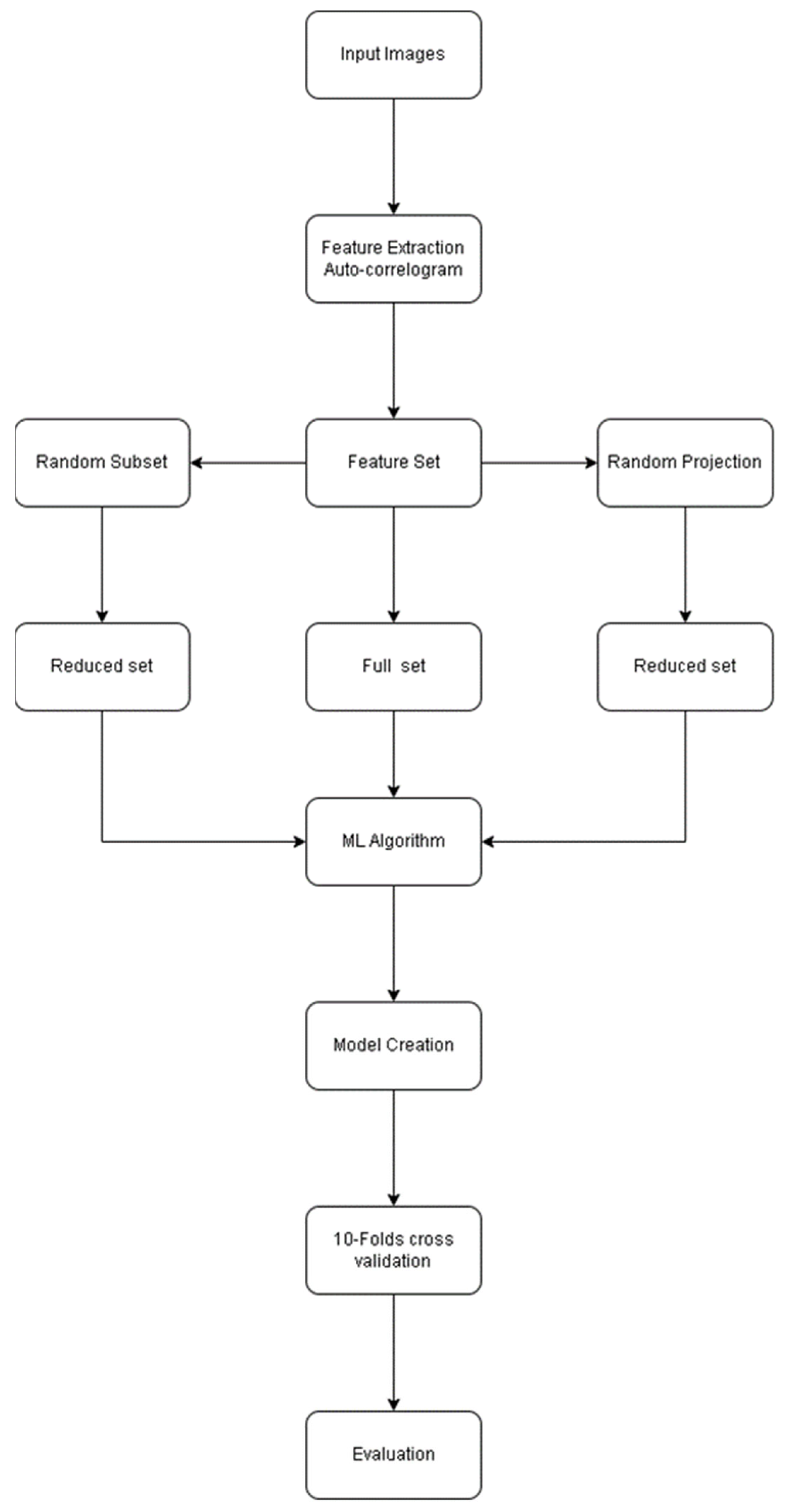
Figure 1. Proposed evaluation methodology.
Electronics 11 03177 g001
The random subset and random projection can be further used to extract the desired amount of data starting from 10% to 90%. A 100% selection will mean the actual amount of data. Therefore, we do not need to extract the 100% set because it is already available as a full set in Figure 1.
The output of previous steps is thus a reduced or full feature set that the classifiers can use for evaluation. The classifier selected (in the ML algorithm block) is used to learn a model from the features extracted in the previous steps. We employ the two classifiers, Naïve Bayesian and the Bayesian Network, for experimental evaluation and the proof of concepts. We selected probabilistic models, including Naïve Bayesian and Bayesian networks, due to their feasibility for feature independence. The Naïve Bayesian also has the advantage that it can be incrementally trained and tested for large datasets. It is thus an updatable classifier that is optimal for real-time and large sets of data that cannot be loaded entirely into the memory. We believe that the selection of the two machine learning algorithms, Naïve Bayesian and the Bayesian Network, optimally address our proposed evaluation’s theme.
Once a model is learned, 10-fold cross-validation ensures that the model performance is more robust and can apply to real-world data. The performance reported in all the experiments is an average of 10-fold. The experimental evaluation section explains the evaluation of full sets and reduced sets by the random subset and random projection.

2.1. Naïve Bayesian

Naïve Bayes is a type of supervised learning for classification based on the Bayesian Theorem. Naïve Bayes takes its concept on the assumption that there is no relation between the existence and non-existence of one feature over another. It uses the maximum likelihood technique to estimate a parameter. For a set of attributes X: A1, A2, A3, and A4, the classification function F (X) assumes that the attributes have no parent except C, the primary parent in Naïve Bayes [15] shown in Figure 2. In Naïve Bayes, all the attributes may or may not depend on each other and are equally essential for the model. The technique can generate an estimation based on little data input for training. Depending upon the characteristics of the probability model, the classifier with the most significant value leads the hypothesis. The Naive Bayes classifiers are efficient in many complex real-world situations, despite having a basic design and oversimplified assumptions.

2.2. Bayesian Network

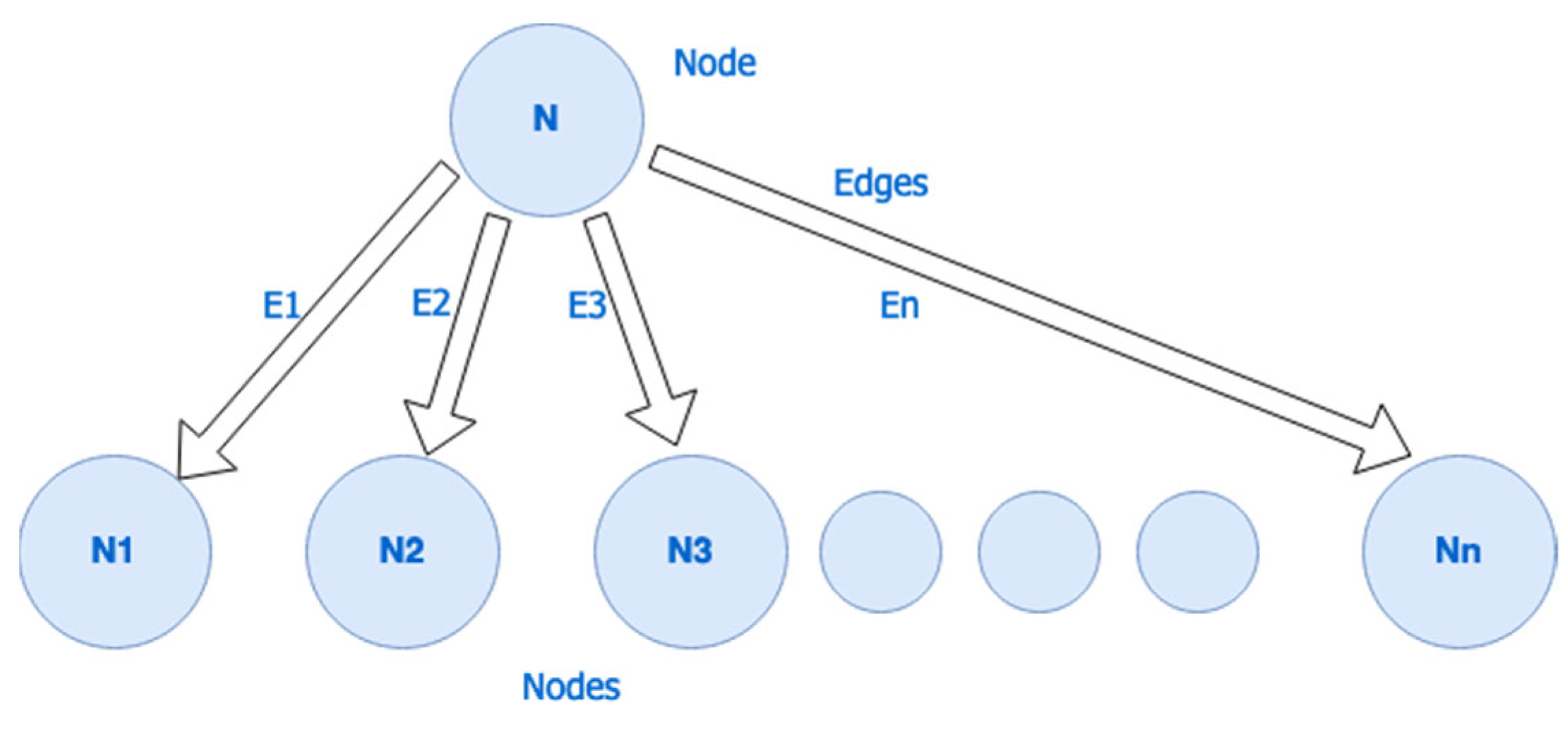
The Bayesian Network has the same assumptions as Naïve Bayes, such as there is no relation between the existence and non-existence of one feature over another [15]. The pictorial illustration of the Bayes Network is provided in Figure 3. The Bayes net structure comprises a root node N, leaves (N1, N2, …, Nn), and the edges (E1, E2, …, En). The nodes can be represented as random variables, which are observable quantities. The edges represent the conditional dependencies, and the leaves represent the hypothesis of the given problem. The network explores all the possible edge combinations to attain an optimal model in the form of an acyclic graph for a given problem statement. The learning process of the Bayesian Network has two stages; the first stage is learning a network structure, and the second is learning the probability tables. Many efficient algorithms perform inference and learning in Bayesian networks.

3. Experimental Evaluation

3.1. Rational

We employ the two classifiers, Naïve Bayesian and the Bayesian Network, for experimental evaluation and the proof of concepts. We selected probabilistic models, including Naïve Bayesian and Bayesian networks, due to their feasibility for feature independence. The Naïve Bayesian also has the advantage that it can be incrementally trained and tested for large datasets. It is thus an updatable classifier that is optimal for real-time and large sets of data that cannot be loaded entirely into the memory. We believe that the selection of the two machine learning algorithms, Naïve Bayesian and the Bayesian Network, optimally addresses the experimental evaluation’s theme.

3.2. Dataset

For experimental evaluation, the NDPI large video dataset [23] is used and divided into three categories: acceptable, flagged, and unacceptable data for analysis. The data from image filtering is utilized for data sampling. The data used are well organized due to three reasons, i.e., they are well categorized into three categories, the data can be converted into numerical representations, and a large amount of data, up to 40 GB, is available, which makes a case for large data processing and thus appropriate for comprehensive machine learning-based analysis.

3.3. Experimental Setup

The experiments of this study aim to analyze the influence of different techniques on the model performance by combining feature selection techniques and machine learning classifiers. The features are extracted using the autocorrelogram approach. The autocorrelogram approach considers color and texture and caters to the spatial arrangements in the image. To evaluate smaller and large sets, two feature selection techniques are used in the experiments; random subset and random projection. Two machine learning classifiers were used as well; Naïve Bayes and Bayesian Network. Our experiment approach maximizes the model performance by reducing the data dimensionality. Table 1 presents the four combinations of feature selection techniques and machine learning classifiers.
In each combination of the experiments, ten rounds were performed. The first round used the entire dataset. In each subsequent round, the dataset is reduced by 10% using the feature selection technique. The last round used only 10% of the original dataset. The run was repeated ten times in each round, and the average performance was recorded. With a total number of 400 runs, the goal was to avoid any biased or chance results. Repeating the runs and taking the average performance provides more confidence in the performance evaluation of the model. In each run, 90% of the data were used for training the classifier and 10% for testing the generated model. In the following figures, 40 average performance values were recorded for the four different combinations of the experiments and are explained in the next section.

4. Evaluation, Results, and Discussion

In the first combination of the experiments (Table 2), the random subset technique and the Naïve Bayes classifier were used. Starting with the entire dataset repeated for ten-time runs and taking the average performance, further similar nine rounds have the same scenario by reducing the dataset by 10% in each round, reaching the last round with only 10% of the original dataset. The measurement of accuracy used for evaluating the generated model’s performance is F-measure, calculated in each round.
The F-measure of the first round, called the base round, where the original dataset was used in the experiment, is 0.721. Commonly, it is thought that the F-measure of 100% of the dataset would result in the best performance among all the other rounds of combination 1 experiments. However, this is not the case, at least for combination 1 experiments. With an overall look at the performances of the ten rounds, it is clear that the best F-measure value goes for the third round, where 80% of the dataset was used. The F-measure for this round is 0.729. This result highlights the advantage of the random subset reduction approach.
Interestingly, the performance in this round, where only 80% of the dataset was used, is better than the performance of the base round, where the full dataset was used. Although the difference in the performance between the two rounds is slight, it reduces the processing resources. It makes an interesting remark about the potential of using sampling approaches for big data processing. The F-measure for the rest of the rounds ranges between 0.727 in the sixth round and 0.693 in the ninth round, where the model’s performance is at the bottom. The most interesting outcome of the combination 1 experiments is that three rounds have the same performance, rounds one, two, and ten. It is worth mentioning that the base round that uses the full data set has the same performance as the tenth round, where only 10% of the original dataset is used. When comparing the amount of two sets of data used for these two rounds, a massive reduction in processing resources has been made with the same model performance. Again, this is not always the case, but at least this combination of the experiments proves that the 90% reduction of the dataset did not affect the model’s performance. In other words, sampling the data can add advantages to big data processing by reducing the processing resources and increasing the accuracy of the generated model in some cases. Figure 4 shows the F-measure for Naïve Bayesian with a random subset.
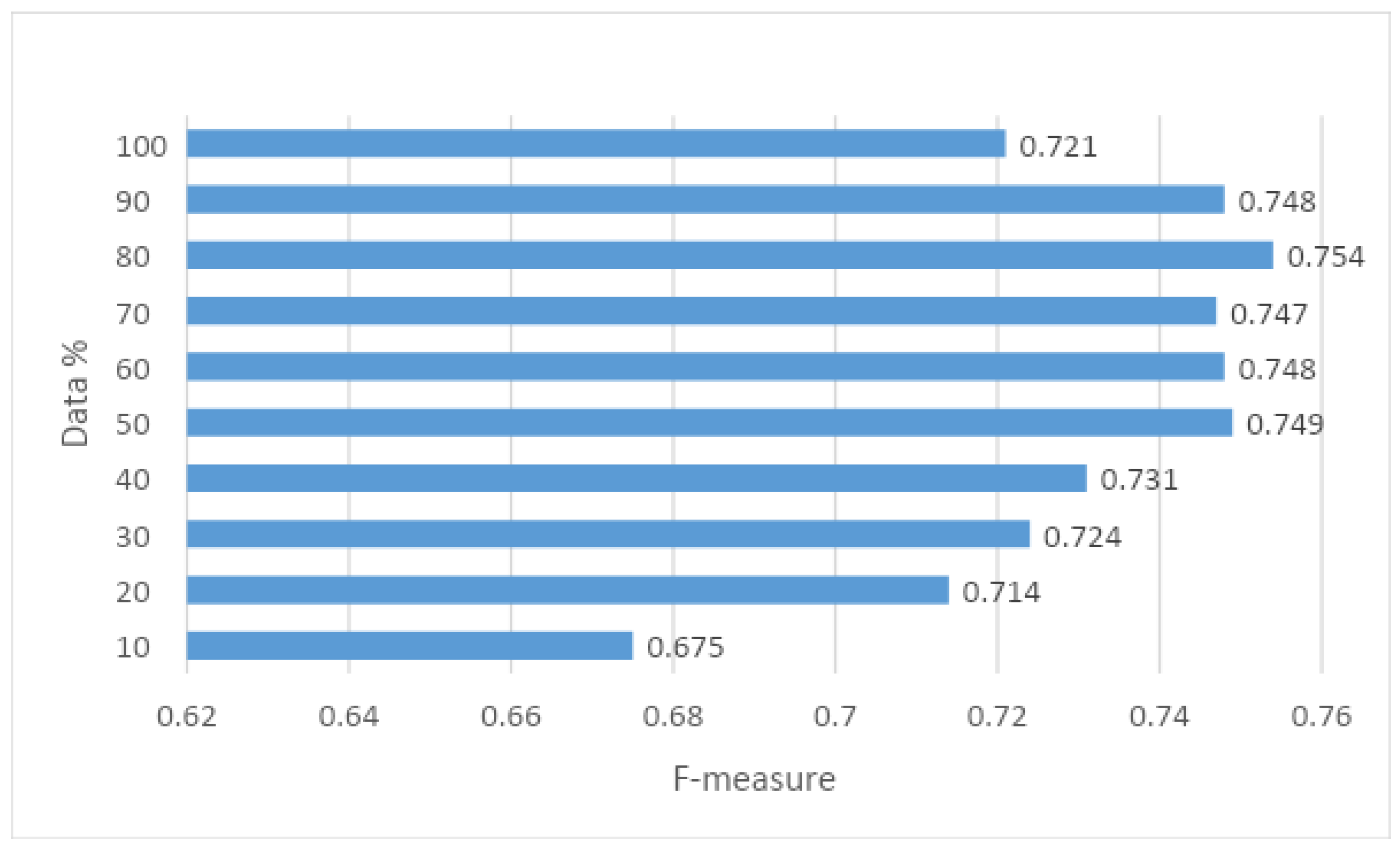
In the second combination (Table 3), the random projection technique and the Naïve Bayes classifier were used.
In the first round, where the full dataset was used, the F-measure for the generated model was 0.721. Assuming that the entire dataset would result in the best performance among all rounds since the whole dataset was used, the second round, where 90% of the dataset was used, recorded a better performance at 0.748. Looking at the third round that uses 80% of the dataset, the performance becomes even the best among all the rounds of this combination, where the F-measure has the value of 0.754. This raised a question about the need for using the full dataset for big data analytics, where sampling can provide even better performance of the model and fewer processing resources used. Again, similar to combination 1, the best performance in this combination was recorded for the third round, where 80% of the dataset was used. This is an indication but not a conclusion about the best setting for the Naïve Bayes classifier when using the random subset and projection techniques to reduce the dataset to 80% of the original collection. The performance of the rest of the rounds ranges between 0.749 in the sixth round and 0.675 in the tenth round, where the model’s performance is at the bottom. It is worth mentioning that the worst performance was recorded when only 10% of the dataset was used. This could indicate that reducing the dataset to this amount results in missing some valuable data. While sampling techniques could provide valuable improvements to big data processing, the threshold of reducing the amount of data is another factor that needs to be investigated in detail. While the performance improved in the fifth and sixth rounds, it drops down afterward in each round with an inverse relation to the amount of the dataset reduced. Again, this can prove that it is not necessary to improve the performance by reducing the dataset but to understand the nature of the data and the sampling technique used to reach the optimal reducing amount that provides the best performance for the generated model of the classifier. Thus, it is a multi-faced methodology that the decision-maker must consider when processing big data. Figure 5 shows the F-measure for Naïve Bayesian with a random projection.
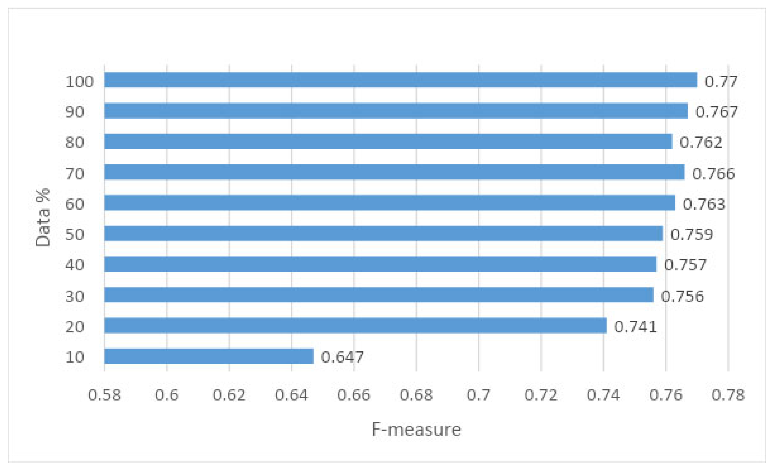
In the third combination (Table 4), the random subset technique and the Bayesian network classifier were used. Unlike the previous two combinations, the best performance recorded for this combination was in the first round, where the full dataset was used.
The F-measure for the first round is 0.77, which decreases afterward to 0.767 in the second round, where 90% of the dataset was used, and 0.762 in the third round, where 80% of the dataset was used. The F-measure returned to increase again at 0.766 in the fourth round. However, it kept decreasing slightly afterward until the ninth round, where the performance at that point was 0.741. A sharp drop was recorded for the tenth round at 0.647, where only 10% of the dataset was used. The scenario in this combination has a different behavior than the previous two experiment combinations. The random subset technique has not provided advantages to the classifier’s performance. However, one can conclude that with the slight decrease in the performance of the generated model, it is worth the great deal of the reduction in the dataset amount, the thing that the decision-maker can decide given that the sampling technique would provide an improvement concerning the processing resources used. Figure 6 shows the F-measure for Bayesian Network with a random subset.
In the fourth combination (Table 5), the random projection technique and the Bayesian network classifier were used.
Similar to the third combination, the best performance was recorded in the first round with an F-measure value of 0.77. The performance afterward fluctuated, with slight ups and downs between 0.748 in the third round and 0.72 in the ninth round. The worst performance was recorded in the tenth round at 0.672, where only 10% of the dataset was used. It can be inferred from this combination that the random projection technique did not improve the performance of the generated model. However, looking at the slight decrease in the performance with the dramatic saving on processing resources by reducing the amount of dataset, one can point out that the sampling technique provided an advantage of reducing the resources used. Figure 7 shows the F-measure for Bayesian Network with a random projection.
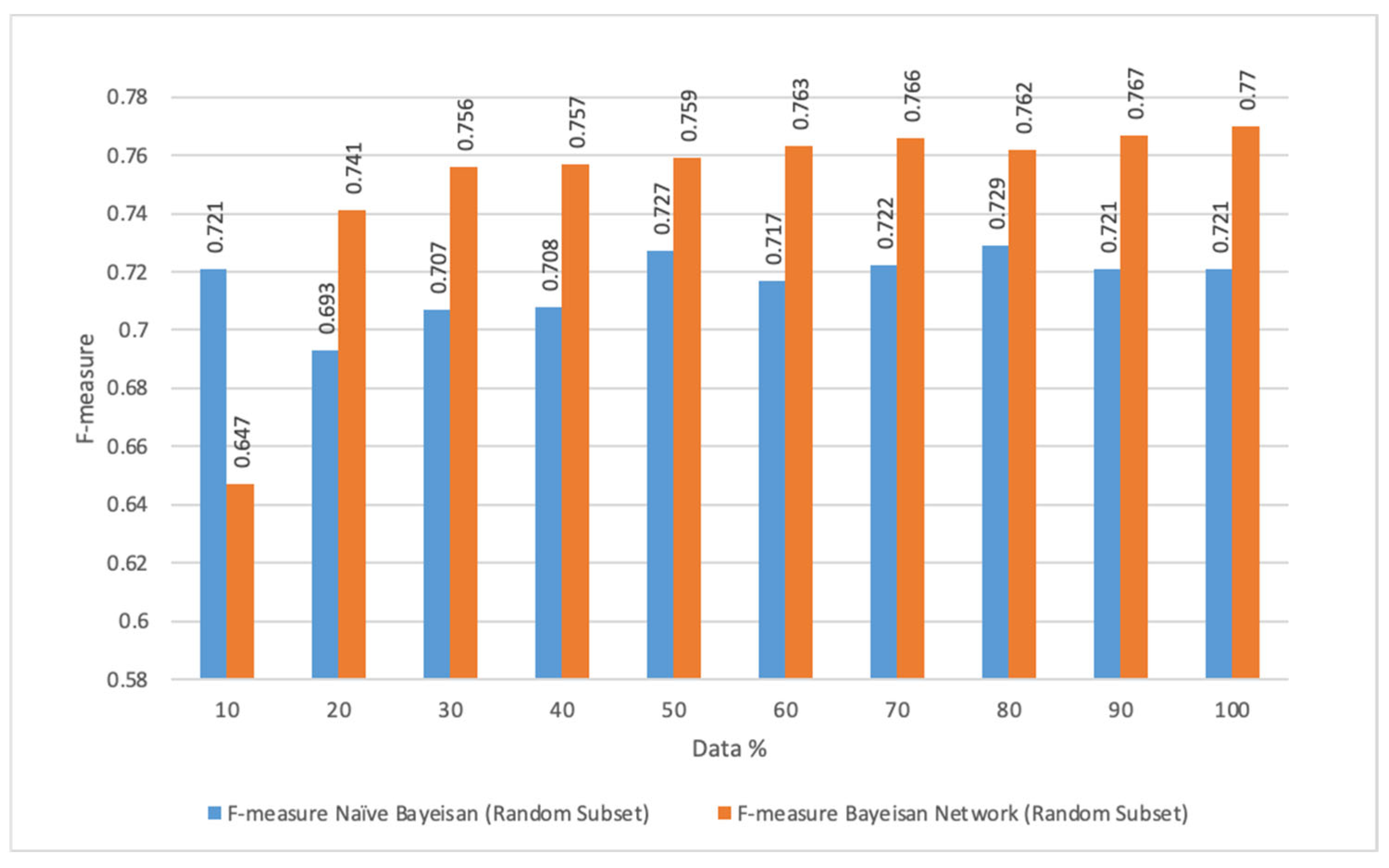
Figure 8 and Figure 9 show the comparative F-measures for the Naïve Bayesian and the Bayesian Network for random subset and the random projection approaches. Figure 8 shows the random subset F-measure distribution for the two classifiers. In Figure 8, we can see that the overall model accuracy of the Bayesian network is higher than the Naïve Bayesian. Initially, with 10% data, the Naïve Bayesian has higher accuracy, but as the data increases, the Naïve Bayesian is outperformed by the Bayesian Network. With the data increase per scenario, the Bayesian Network receives approximately a 5% increase in performance. Figure 9 shows the random projection F-measure for the two classifiers. Figure 9 indicates that the Bayesian network in many rounds still outperforms the Naïve Bayesian, but the influence is not as dominant as that of Figure 8.
Figure 10 summarizes the overall statistics in one graph. With the overall view of Figure 10, the best performance among all combinations is recorded for combination 3, where the random subset technique and the Bayesian network classifier were used. Except for the round where 10% of the dataset was used, combination 1 has the best performance among all combinations.

5. Comparative Analysis

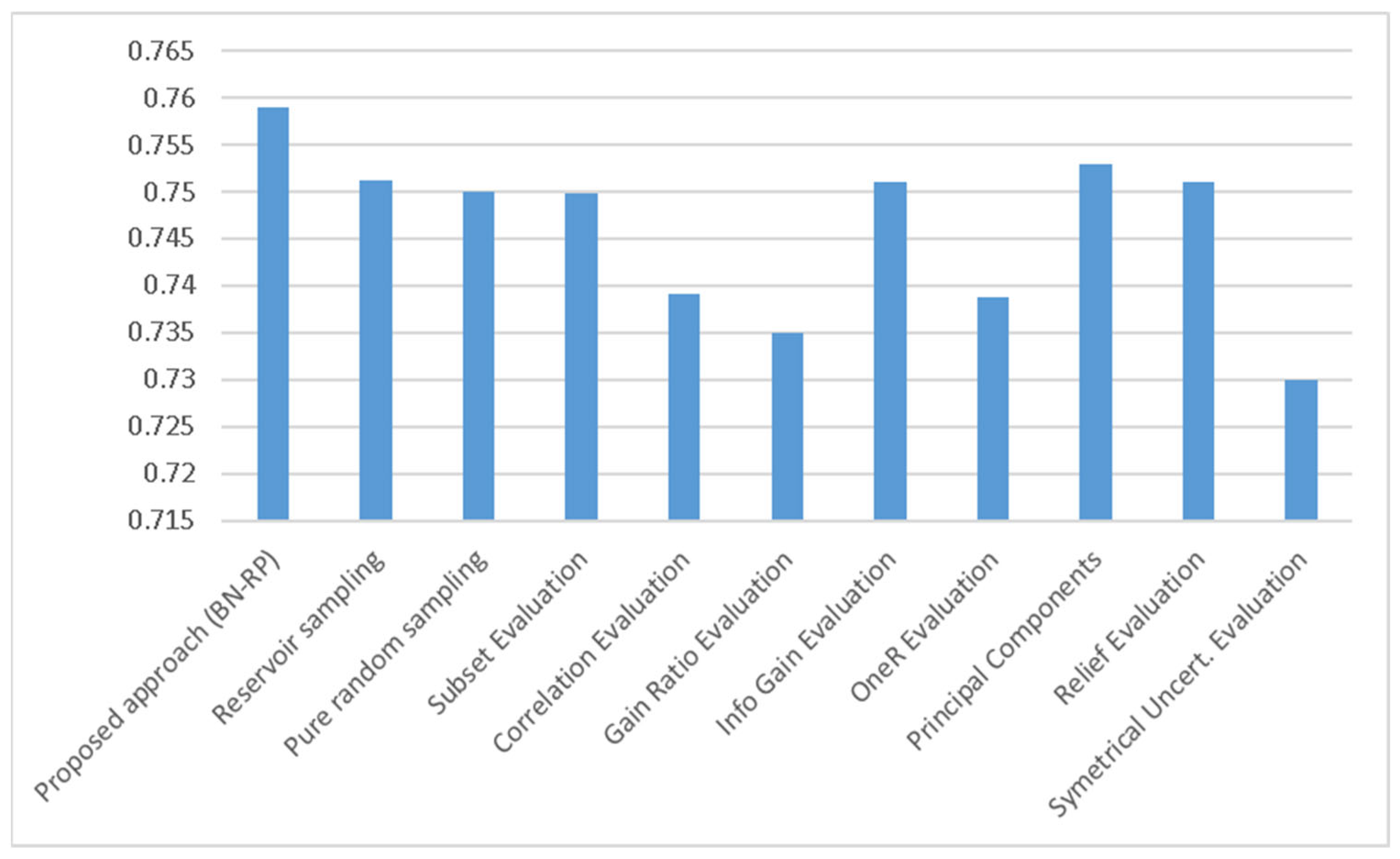
For comparison, we include experiments covering different approaches that have similar feature/data extraction capabilities. For the comparison, we fix (select) the proposed Bayesian with Random Projection, represented as BN-RP. By selection here, we mean that since there are many permutations in this article, we select one good performance setting for our evaluation. We fix the 50% data as the baseline for all the feature/data selection approaches. For the comparison, we use reservoir sampling [8], Pure random sampling, and Subset-Eva. [41], Correlation Eval. [63], Gain-R [19], Info-Gain [20], OneR [43], PCA [44], Relief [45], and Symmetrical-Uncertain-Evaluation [64]. These are among the widely used features/data selection approaches in the state of the art. We have used similar settings for all the feature/data extraction approaches. These are among the most widely used features/data selection approaches in the state of the art. We have used similar settings for all the feature/data extraction approaches.
Table 6 and Figure 11 show the details comparison of the different approaches based on the F-measure. The proposed approach has the highest F-measure of 0.759. The reservoir sampling achieves an F-measure of 0.751. Pure random sampling achieves an F-measure of 0.749. Pure random sample here refers to an approach that takes the first 50% of the data if arranged in order. The subset evaluation has almost similar performance to that of pure random sampling. The correlation evaluation and gain ratio have almost similar F-measures. The info gain, PCA, and relief evaluations have a good F-measure of over 0.75. The OneR and info gain evaluations reduced the F-measure to 0.73. Thus, the proposed approach outperforms all the other approaches.

6. Conclusions

Big data analytics is still a challenging process in both levels of data processing and computing resources. This study has analyzed a large amount of data with classical machine learning. As such, the main objective of this article was to show that in large datasets, it is quite possible that a random selection of features can be as good as the selection of features by optimization algorithms such as the Pareto-front, ant colony optimization, particle swarm optimization, and many others. Thus, this study has analyzed a large amount and sampled it randomly into subsets. The influence of different techniques on the model performance is analyzed by combining the feature selection techniques and machine learning classifiers. The experiments used two feature selection techniques: random subset and random projection. In the evaluation, it was noted that the overall performance fluctuates between 70% accuracy to 74% accuracy for using sampled and non-sampled (all the data). Thus, in large datasets, it is quite possible that the random selection of the small portion of the data can produce as good results as the original data. The difference in performance is only slightly over 3%, which is negligible. We thus argue that if optimized algorithms are used, the performance will still be the same because the actual performance of 100% data differs very little from the reduced data samples. Thus, we argue that whether or not the reduced samples are selected by optimization algorithms such as the Pareto-front, ant-colony, particle swarm optimization, and many others, their performance will be the same or close because, with sampled versions, we should not be able to outperform the model of the 100% data.

Author Contributions

Conceptualization, R.U.K. and W.A.; Formal analysis, R.U.K.; Funding acquisition, M.F.A.; Methodology, R.U.K.; Project administration, W.A.; Supervision, M.F.A.; Writing—original draft, W.A. and R.U.K.; Writing—review & editing, W.A. and S.F.K. All authors have read and agreed to the published version of the manuscript.

Funding

This research received no external funding.

Institutional Review Board Statement

Not applicable.

Informed Consent Statement

Not applicable.

Data Availability Statement

Not applicable.

Acknowledgments

The researcher(s) would like to thank the Deanship of Scientific Research, Qassim University for funding the publication of this project.

Conflicts of Interest

The authors declare no conflict of interest.

References

  1. Albattah, W. The role of sampling in big data analysis. In Proceedings of the International Conference on Big Data and Advanced Wireless Technologies, Blagoevgrad, Bulgaria, 10 November 2016; pp. 1–5. [Google Scholar]
  2. Hilbert, M. Big data for development: A review of promises and challenges. Dev. Policy Rev. 2016, 34, 135–174. [Google Scholar] [CrossRef] [Green Version]
  3. Reed, D.A.; Dongarra, J. Exascale computing and big data. Commun. ACM 2015, 58, 56–68. [Google Scholar] [CrossRef]
  4. L’Heureux, A.; Grolinger, K.; Elyamany, H.F.; Capretz, M.A.M. Machine learning with big data: Challenges and approaches. IEEE Access 2017, 5, 7776–7797. [Google Scholar] [CrossRef]
  5. Singh, K.; Guntuku, S.C.; Thakur, A.; Hota, C. Big data analytics framework for peer-to-peer botnet detection using random forests. Inf. Sci. 2014, 278, 488–497. [Google Scholar] [CrossRef]
  6. Clarke, R. Big data, big risks. Inf. Syst. J. 2016, 26, 77–90. [Google Scholar] [CrossRef]
  7. Sullivan, D. Introduction to Big Data Security Analytics in the Enterprise. Available online: https://searchsecurity.techtarget.com/feature/Introduction-to-big-data-security-analytics-in-the-enterprise (accessed on 25 May 2021).
  8. Tsai, C.-W.; Lai, C.-F.; Chao, H.-C.; Vasilakos, A.V. Big data analytics: A survey. J. Big Data 2015, 2, 21. [Google Scholar] [CrossRef] [Green Version]
  9. Bello-Orgaz, G.; Jung, J.J.; Camacho, D. Social big data: Recent achievements and new challenges. Inf. Fusion 2016, 28, 45–59. [Google Scholar] [CrossRef]
  10. Zakir, J.; Seymour, T.; Berg, K. Big data analytics. Issues Inf. Syst. 2015, 16, 81–90. [Google Scholar]
  11. Sivarajah, U.; Kamal, M.M.; Irani, Z.; Weerakkody, V. Critical analysis of big data challenges and analytical methods. J. Bus. Res. 2017, 70, 263–286. [Google Scholar] [CrossRef] [Green Version]
  12. Engemann, K.; Enquist, B.J.; Sandel, B.; Boyle, B.; Jørgensen, P.M.; Morueta-Holme, N.; Peet, R.K.; Violle, C.; Svenning, J.-C. Limited sampling hampers ‘big data’ estimation of species richness in a tropical biodiversity hotspot. Ecol. Evol. 2015, 5, 807–820. [Google Scholar] [CrossRef]
  13. Kim, J.K.; Wang, Z. Sampling techniques for big data analysis. Int. Stat. Rev. 2018, 87, S177–S191. [Google Scholar] [CrossRef]
  14. Liu, S.; She, R.; Fan, P. How many samples required in big data collection: A differential message importance measure. arXiv 2018, arXiv:1801.04063. [Google Scholar]
  15. Bierkens, J.; Fearnhead, P.; Roberts, G. The zig-zag process and super-sufficient sampling for Bayesian analysis of big data. Ann. Stat. 2016, 47, 1288–1320. [Google Scholar]
  16. Zhao, J.; Sun, J.; Zhai, Y.; Ding, Y.; Wu, C.; Hu, M. A novel clustering-based sampling approach for minimum sample set in big data environment. Int. J. Pattern Recognit. Artif. Intell. 2018, 32, 1850003. [Google Scholar] [CrossRef]
  17. Zhou, L.; Pan, S.; Wang, J.; Vasilakos, A.V. Machine learning on big data: Opportunities and challenges. Neurocomputing 2017, 237, 350–361. [Google Scholar] [CrossRef] [Green Version]
  18. Kotzias, D.; Denil, M.; de Freitas, N.; Smyth, P. From group to individual labels using deep features. In Proceedings of the 21th ACM SIGKDD International Conference on Knowledge Discovery and Data Mining, Sydney, Australia, 10 August 2015; pp. 597–606. [Google Scholar]
  19. Karegowda, A.G.; Manjunath, A.S.; Jayaram, M.A. Comparative study of attribute selection using gain ratio and correlation based feature selection. Int. J. Inf. Technol. Knowl. Manag. 2010, 2, 271–277. [Google Scholar]
  20. Holte, R.C. Very simple classification rules perform well on most commonly used datasets. Mach. Learn. 1993, 11, 63–90. [Google Scholar] [CrossRef]
  21. Farabet, C.; Couprie, C.; Najman, L.; LeCun, Y. Learning hierarchical features for scene labeling. IEEE Trans. Pattern Anal. Mach. Intell. 2013, 35, 1915–1929. [Google Scholar] [CrossRef] [PubMed] [Green Version]
  22. Krizhevsky, A.; Sutskever, I.; Hinton, G.E. ImageNet classification with deep convolutional neural networks. In Proceedings of the International Conference on Neural Information Processing Systems, Lake Tahoe, NV, USA, 24 May 2012; Volume 1, pp. 1097–1105. [Google Scholar]
  23. Avila, S.; Thome, N.; Cord, M.; Valle, E.; de Araújo, A. Pooling in image representation: The visual codeword point of view. Comput. Vis. Image Underst. 2013, 117, 453–465. [Google Scholar] [CrossRef]
  24. Moustafa, M.N. Applying deep learning to classify pornographic images and videos. In Proceedings of the 7th Pacific-Rim Symposium on Image and Video Technology (PSIVT 2015), Auckland, New Zealand, 28 November 2015. [Google Scholar]
  25. Lopes, A.P.B.; de Avila, S.E.F.; Peixoto, A.N.A.; Oliveira, R.S.; de Coelho, M.; Araújo, A.D.A. Nude detection in video using bag-of-visual-features. In Proceedings of the 2009 XXII Brazilian Symposium on Computer Graphics and Image Processing, Rio de Janeiro, Brazil, 11–15 October 2009; pp. 224–231. [Google Scholar]
  26. Abadpour, A.; Kasaei, S. Pixel-based skin detection for pornography filtering. Iran. J. Electr. Electron. Eng. 2005, 1, 21–41. [Google Scholar]
  27. Ullah, R.; Alkhalifah, A. Media content access: Image-based filtering. Int. J. Adv. Comput. Sci. Appl. 2018, 9, 415–419. [Google Scholar] [CrossRef] [Green Version]
  28. Szegedy, C.; Liu, W.; Jia, Y.; Sermanet, P.; Reed, S.; Anguelov, D.; Erhan, D.; Vanhoucke, V.; Rabinovich, A. Going deeper with convolutions. In Proceedings of the 2015 IEEE Conference on Computer Vision and Pattern Recognition (CVPR), Boston, MA, USA, 7–12 June 2015; pp. 1–9. [Google Scholar]
  29. Valle, E.; Avila, S.; de Souza, F.; Coelho, M.; de Araújo, A. Content-based filtering for video sharing social networks. In Proceedings of the XII Simpósio Brasileiro em Segurança da Informação e de Sistemas Computacionais—SBSeg, Curitiba, Brazil, 12 January 2011; p. 28. [Google Scholar]
  30. da Silva Eleuterio, P.M.; de Castro Polastro, M. An adaptive sampling strategy for automatic detection of child pornographic videos. In Proceedings of the Seventh International Conference on Forensic Computer Science, Brasilia, Brazil, 24 September 2012; pp. 12–19. [Google Scholar]
  31. Agarwal, N.; Liu, H.; Zhang, J. Blocking objectionable web content by leveraging multiple information sources. ACM SIGKDD Explor. Newsl. 2006, 8, 17–26. [Google Scholar] [CrossRef]
  32. Jansohn, C.; Ulges, A.; Breuel, T.M. Detecting pornographic video content by combining image features with motion information. In Proceedings of the Seventeen ACM International Conference on Multimedia—MM, Beijing, China, 19–22 October 2009; p. 601. [Google Scholar]
  33. Wang, J.-H.; Chang, H.-C.; Lee, M.-J.; Shaw, Y.-M. Classifying peer-to-peer file transfers for objectionable content filtering using a web-based approach. IEEE Intell. Syst. 2002, 17, 48–57. [Google Scholar]
  34. Lee, H.; Lee, S.; Nam, T. Implementation of high performance objectionable video classification system. In Proceedings of the 2006 8th International Conference Advanced Communication Technology, Phoenix Park, Korea, 20–22 February 2006; pp. 962–965. [Google Scholar]
  35. Liu, D.; Hua, X.-S.; Wang, M.; Zhang, H. Boost search relevance for tag-based social image retrieval. In Proceedings of the 2009 IEEE International Conference on Multimedia and Expo, New York, NY, USA, 28 June–3 July 2009; pp. 1636–1639. [Google Scholar]
  36. da Silva Júnior, J.A.; Marçal, R.E.; Batista, M.A. Image retrieval: Importance and applications. In Proceedings of the Workshop de Visao Computacional—WVC, Uberlandia, Brazil, 6–8 October 2014. [Google Scholar]
  37. Badghaiya, S.; Barve, A. Image classification using tag and segmentation based retrieval. Int. J. Comput. Appl. 2014, 103, 20–23. [Google Scholar] [CrossRef]
  38. Bhute, A.N.; Meshram, B.B. Text based approach for indexing and retrieval of image and video: A review. Adv. Vis. Comput. Int. J. 2014, 1, 27–38. [Google Scholar] [CrossRef] [Green Version]
  39. Cortes, C.; Vapnik, V. Support-Vector Networks. Mach. Learn. 1995, 20, 273–297. [Google Scholar] [CrossRef]
  40. Breiman, L. Random Forests. Mach. Learn. 2001, 45, 5–32. [Google Scholar] [CrossRef] [Green Version]
  41. Hall, M.A.; Smith, L.A. Practical feature subset selection for machine learning. In Proceedings of the 21st Australasian Computer Science Conference ACSC’98, Perth, Australia, 4–6 February 1998; pp. 181–191. [Google Scholar]
  42. Hall, M.A. Correlation-Based Feature Selection for Machine Learning. Ph.D. Thesis, The University of Waikato, Hamilton, New Zealand, 1999. [Google Scholar]
  43. Jolliffe, I.T. Choosing a subset of principal components or variables. In Principal Component Analysis; Springer: New York, NY, USA, 1986; pp. 92–114. [Google Scholar]
  44. Kira, K.; Rendell, L.A. A practical approach to feature selection. Mach. Learn. Proc. 1992, 1992, 249–256. [Google Scholar]
  45. Kononenko, I. Estimating attributes: Analysis and extensions of RELIEF. In Proceedings of the European Conference on Machine Learning, Catania, Italy, 6–8 April 1994; pp. 171–182. [Google Scholar]
  46. Albattah, W.; Khan, R.U. Processing sampled big data. Int. J. Adv. Comput. Sci. Appl. 2018, 9, 350–356. [Google Scholar] [CrossRef] [Green Version]
  47. Albattah, W.; Albahli, S. Content-based prediction: Big data sampling perspective. Int. J. Eng. Technol. 2019, 8, 627–635. [Google Scholar] [CrossRef]
  48. Hastie, T.; Tibshirani, R.; Friedman, J. The Elements of Statistical Learning: Data Mining, Inference, and Prediction, 2nd ed.; Springer: Berlin/Heidelberg, Germany, 2009. [Google Scholar]
  49. Wang, C.; Shi, Y.; Fan, X.; Shao, M. Attribute reduction based on k-nearest neighborhood rough sets. Int. J. Approx. Reason. 2019, 106, 18–31. [Google Scholar] [CrossRef]
  50. Lakshmanaprabu, S.K.; Shankar, K.; Khanna, A.; Gupta, D.; Rodrigues, J.J.P.C.; Pinheiro, P.R.; De Albuquerque, V.H.C. Effective features to classify big data using social internet of things. IEEE Access 2018, 6, 24196–24204. [Google Scholar] [CrossRef]
  51. Reddy, G.T.; Reddy, M.P.K.; Lakshmanna, K.; Kaluri, R.; Rajput, D.S.; Srivastava, G.; Baker, T. Analysis of dimensionality reduction techniques on big data. IEEE Access 2020, 8, 54776–54788. [Google Scholar] [CrossRef]
  52. Chen, H.; Li, T.; Cai, Y.; Luo, C.; Fujita, H. Parallel attribute reduction in dominance-based neighborhood rough set. Inf. Sci. 2016, 373, 351–368. [Google Scholar] [CrossRef] [Green Version]
  53. Li, J.; Yang, X.; Song, X.; Li, J.; Wang, P.; Yu, D.-J. Neighborhood attribute reduction: A multi-criterion approach. Int. J. Mach. Learn. Cybern. 2019, 10, 731–742. [Google Scholar] [CrossRef]
  54. Rostami, M.; Berahmand, K.; Forouzandeh, S. A novel community detection based genetic algorithm for feature selection. J. Big Data 2021, 8, 1–27. [Google Scholar] [CrossRef]
  55. Rajendran, S.; Khalaf, O.I.; Alotaibi, Y.; Alghamdi, S. MapReduce-based big data classification model using feature subset selection and hyperparameter tuned deep belief network. Sci. Rep. 2021, 11, 1–10. [Google Scholar]
  56. Rostami, M.; Berahmand, K.; Nasiri, E.; Forouzandeh, S. Review of swarm intelligence-based feature selection methods. Eng. Appl. Artif. Intell. 2021, 100, 104210. [Google Scholar] [CrossRef]
  57. Song, X.F.; Zhang, Y.; Gong, D.W.; Gao, X.Z. A fast hybrid feature selection based on correlation-guided clustering and particle swarm optimization for high-dimensional data. IEEE Trans. Cybern. 2021, 52, 9573–9586. [Google Scholar] [CrossRef]
  58. Jain, D.K.; Boyapati, P.; Venkatesh, J.; Prakash, M. An intelligent cognitive-inspired computing with big data analytics framework for sentiment analysis and classification. Inf. Process. Manag. 2022, 59, 102758. [Google Scholar] [CrossRef]
  59. Abu Khurma, R.; Aljarah, I.; Sharieh, A.; Abd Elaziz, M.; Damaševičius, R.; Krilavičius, T. A review of the modification strategies of the nature inspired algorithms for feature selection problem. Mathematics 2022, 10, 464. [Google Scholar] [CrossRef]
  60. Dini, P.; Saponara, S. Analysis, design, and comparison of machine-learning techniques for networking intrusion detection. Designs 2021, 5, 9. [Google Scholar] [CrossRef]
  61. Ferrag, M.A.; Friha, O.; Hamouda, D.; Maglaras, L.; Janicke, H. Edge-IIoTset: A New Comprehensive Realistic Cyber Security Dataset of IoT and IIoT Applications for Centralized and Federated Learning. IEEE Access 2022, 10, 40281–40306. [Google Scholar] [CrossRef]
  62. Dini, P.; Begni, A.; Ciavarella, S.; De Paoli, E.; Fiorelli, G.; Silvestro, C.; Saponara, S. Design and Testing Novel One-Class Classifier Based on Polynomial Interpolation with Application to Networking Security. IEEE Access 2022, 10, 67910–67924. [Google Scholar] [CrossRef]
  63. Hall, M. Correlation-based Feature Selection for Machine Learning. Methodology 1999, 21i195-i20, 1–5. [Google Scholar]
  64. Reservoir Sampling—ORIE 6125: Computational Methods in Operations Research 3.0.1 Documentation. 2022. Available online: https://people.orie.cornell.edu/snp32/orie_6125/algorithms/reservoir-sampling.html (accessed on 18 September 2022).
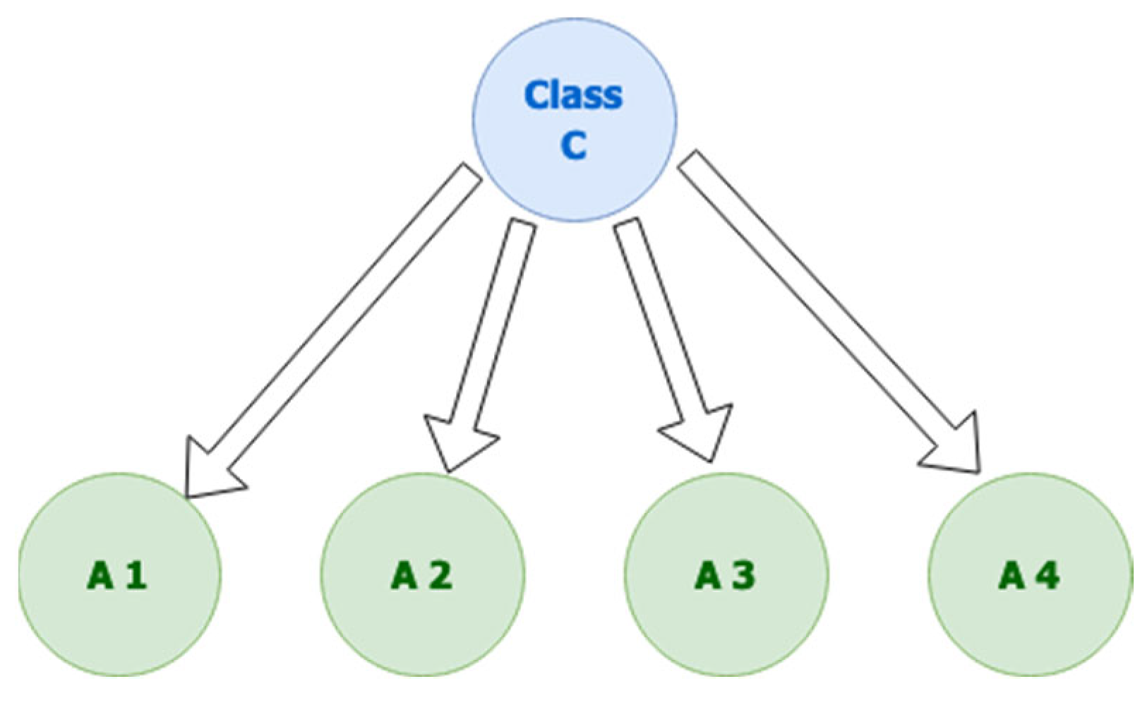
Figure 2. An example of Naïve Bayes.
Electronics 11 03177 g002
Figure 3. An example of Bayes Network.
Electronics 11 03177 g003
Figure 4. F-measure for Naïve Bayesian with a random subset.
Electronics 11 03177 g004
Figure 5. F-measure for Naïve Bayesian with a random projection.
Electronics 11 03177 g005
Figure 6. F-measure for Bayesian Network with a random subset.
Electronics 11 03177 g006
Figure 7. F-measure for Bayesian Network with a random projection.
Electronics 11 03177 g007
Figure 8. Comparative F-measures for Naïve Bayesian and Bayesian Network with a random subset.
Electronics 11 03177 g008
Figure 9. Comparative F-measures for Naïve Bayesian and Bayesian Networks with a random projection.
Electronics 11 03177 g009
Figure 10. Overall F-measure with data samples for the four combinations.
Electronics 11 03177 g010
Figure 11. Comparison of the proposed approach with feature/data selection approaches.
Electronics 11 03177 g011
Table 1. Four combinations of the experiments.
Feature Selection
Random SubsetRandom Projection
ML ModelNaïve BayesCombination 1Combination 2
Bayesian NetworkCombination 3Combination 4
Table 2. F-measure for Naïve Bayesian with a random subset.
PercentageF-Measure Naïve Bayesian (Random Subset)
100.721
200.693
300.707
400.708
500.727
600.717
700.722
800.729
900.721
1000.721
Table 3. F-measure for Naïve Bayesian with a random projection.
PercentageF-Measure Naïve Bayesian (Random Projection)
100.675
200.714
300.724
400.731
500.749
600.748
700.747
800.754
900.748
1000.721
Table 4. F-measure for Bayesian Network with a random subset.
PercentageF-measure Bayesian Network (Random Subset)
100.647
200.741
300.756
400.757
500.759
600.763
700.766
800.762
900.767
1000.77
Table 5. F-measure for Bayesian Network with a random projection.
PercentageF-measure Bayesian Network (Random Projection)
100.672
200.72
300.727
400.742
500.737
600.743
700.738
800.748
900.747
1000.77
Table 6. Comparison of the proposed approach with feature/data selection approaches.
Proposed Approach (BN-RP)0.759
Reservoir sampling0.751222222
Pure random sampling0.749922222
Subset Evaluation0.7498
Correlation Evaluation0.7392
Gain Ratio Evaluation0.735
Info Gain Evaluation0.751
OneR Evaluation0.7387
Principal Components0.753
Relief Evaluation0.751
Symmetrical Uncertain. Evaluation0.73
Publisher’s Note: MDPI stays neutral with regard to jurisdictional claims in published maps and institutional affiliations.