
Hybrid CLAHE-CNN Deep Neural Networks for Classifying Lung Diseases from X-ray Acquisitions

 , , , ,
  and
and 
Abstract
:1. Introduction
2. Literature Review
3. Methodology
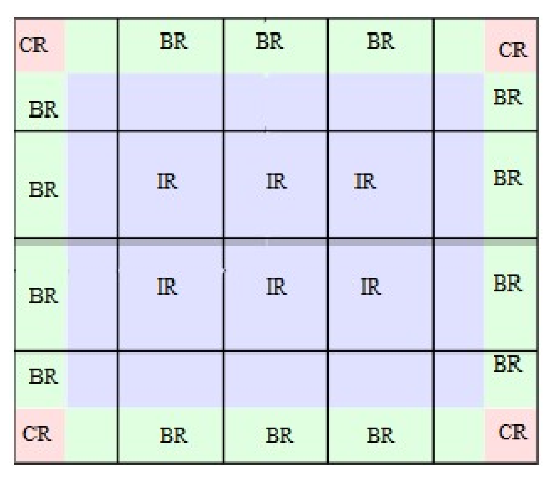
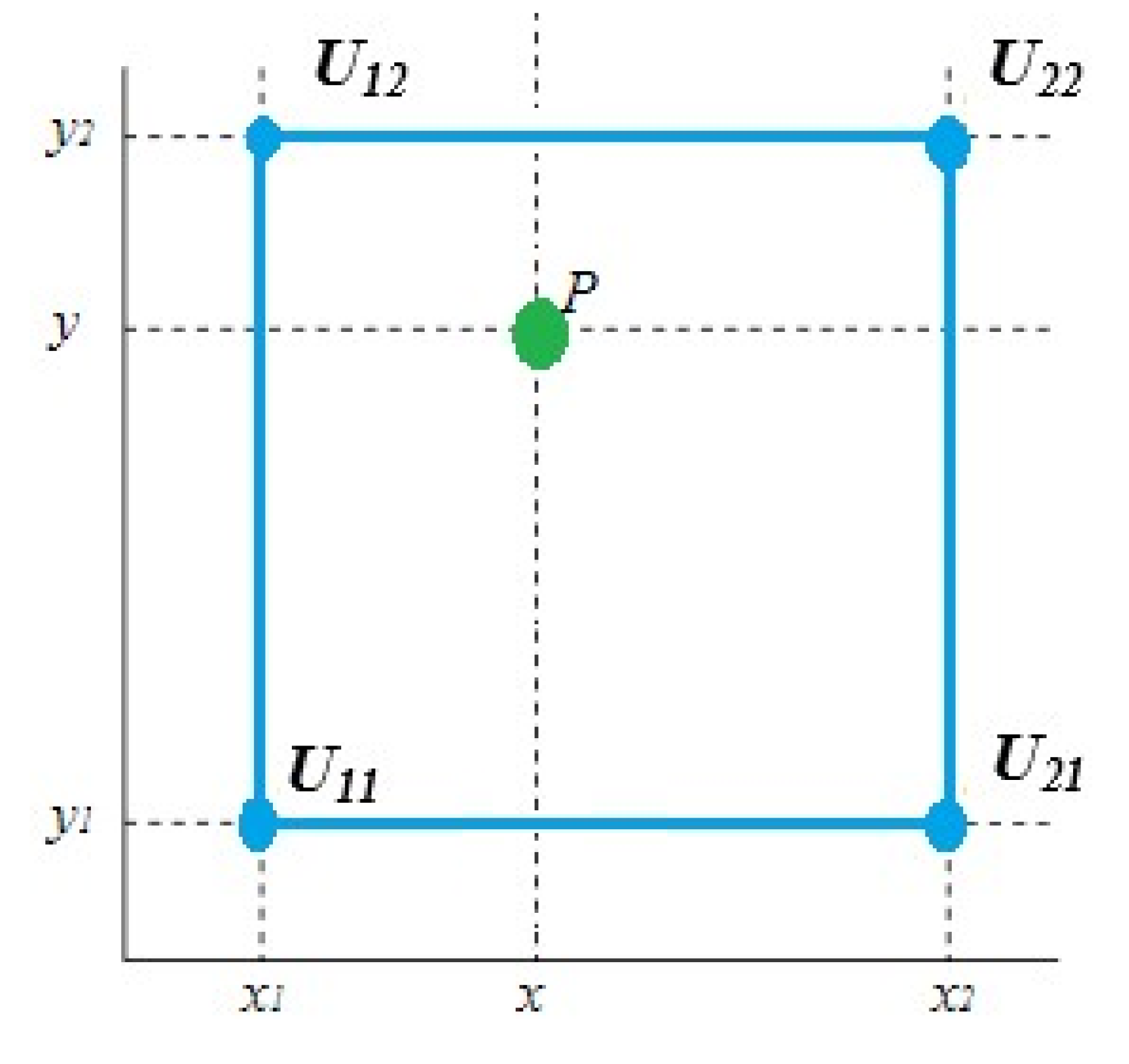
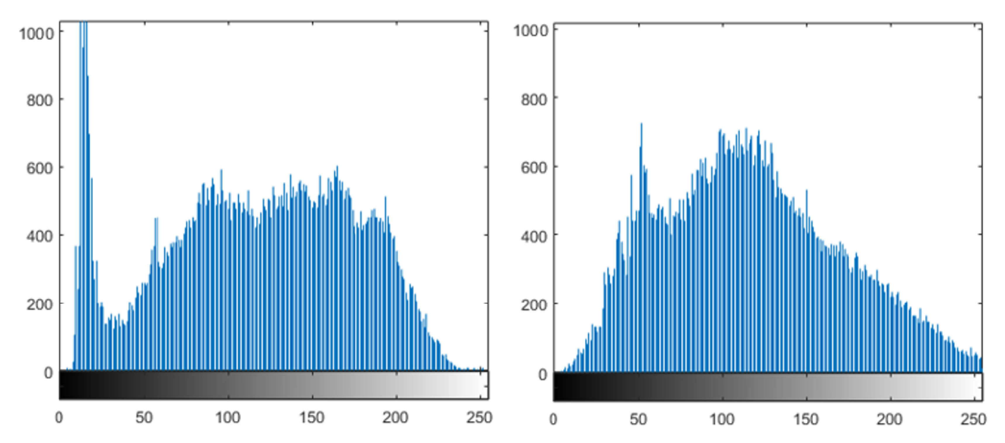
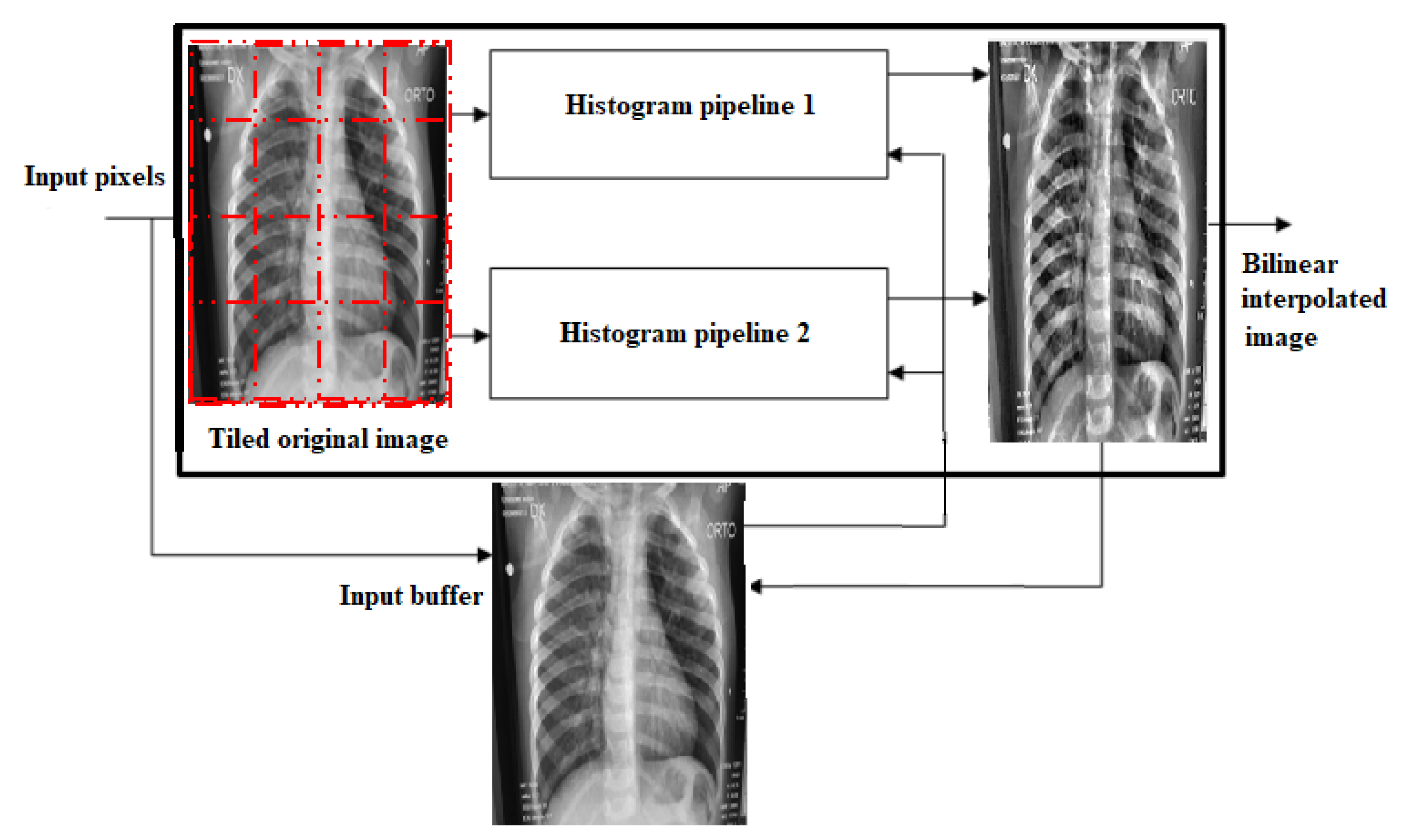
3.1. Preprocessing
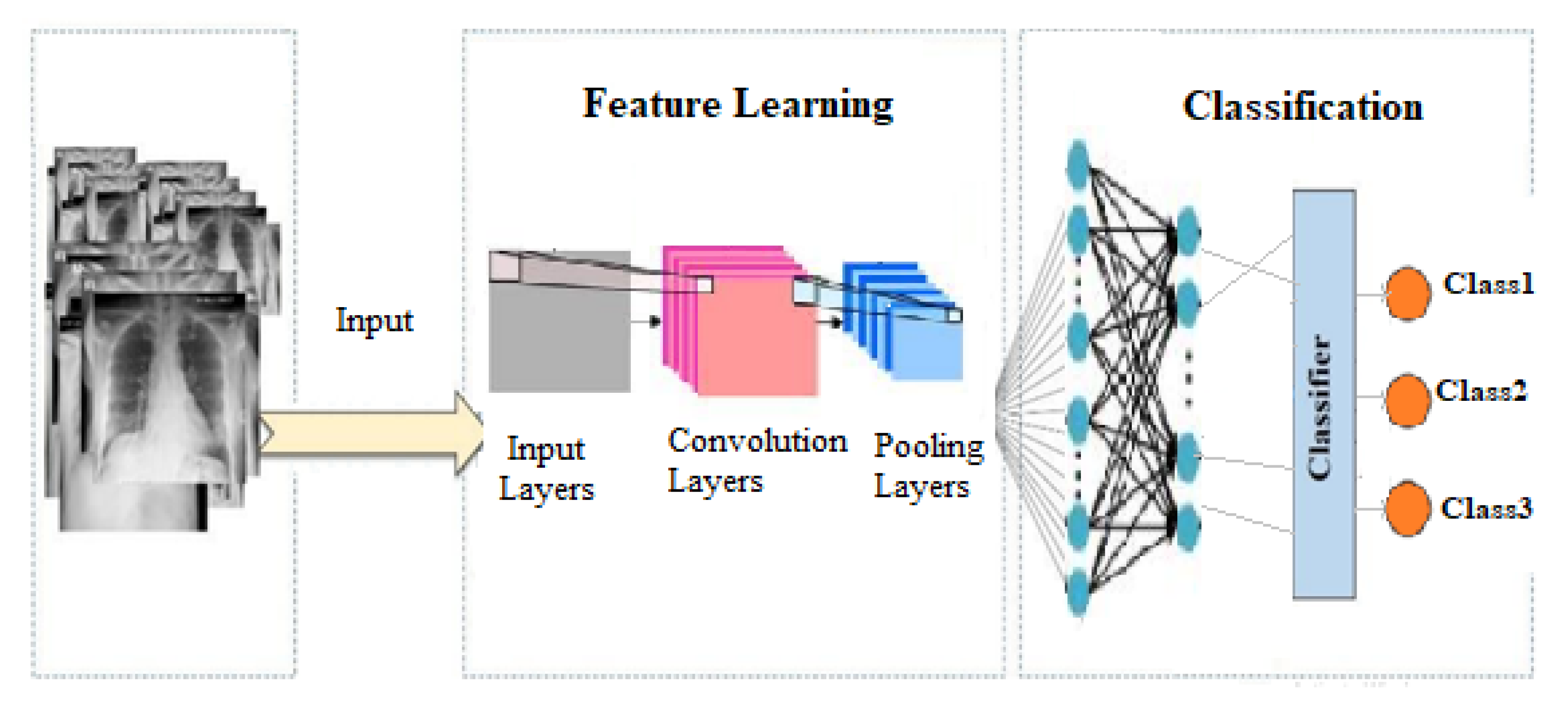
3.2. Proposed System
- Convolution layer: This is the first layer in a CNSN. It blends the input of a matrix of the dimensions and then sends the output to the next layer. Convolution layers are made up of neurons that link to subregions of the input images or the preceding layer’s outputs. Each layer convolves the input by sliding the filters vertically and horizontally along the input. While scanning through an image, the layer learns the features localized by these areas. The image is abstracted to a feature map, also known as an activation map, after the tensor is passed through a convolutional layer.
- Pooling layer: A pooling layer’s main function is to minimize the number of parameters in the input tensor; hence it aids in reducing overfitting, extracts representative features from the input tensor, and reduces computation, which improves efficiency. A pooling layer reduces the amount of parameters that the network must learn by conducting nonlinear sampling on the output. It divides the input into rectangular pooling regions, then computes the maximum of each region. By merging the outputs of neuron clusters at one layer into a single neuron in the following layer, pooling layers minimize the dimensionality of data. It is worth knowing that pooling reduces the image’s height and width while keeping the number of channels (depth) constant.
- Fully connected layer: The convolutional neural network’s last layer is the fully connected layer (also known as the hidden layer). It is a feedforward neural network. The output of the final pooling or convolutional layer is flattened and sent into the fully connected layer. Every neuron in one layer is connected to every neuron in the next layer via fully connected layers. It functions similarly to a standard multilayer perceptron neural network (MLP).
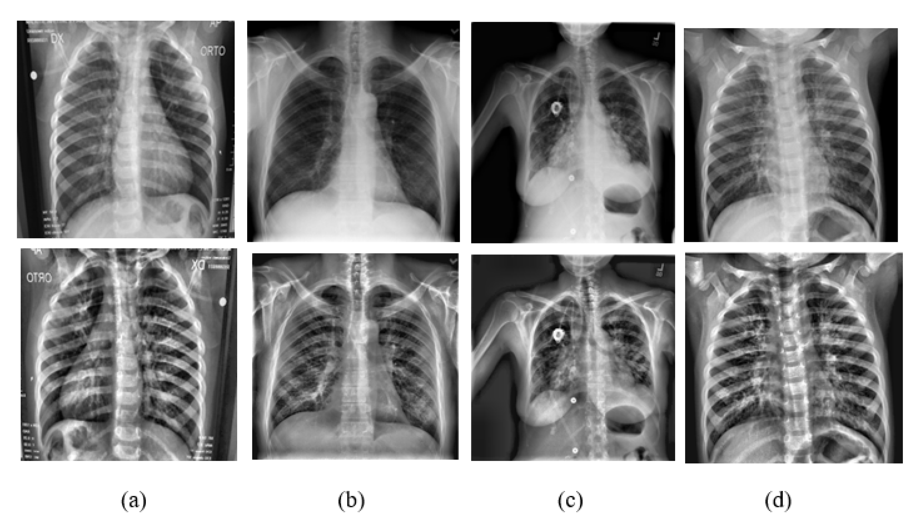
3.3. Dataset
3.4. Algorithm Evaluation
- : The value of the actual class and the value of the predicted class is yes.
- : The value of the actual class and value of the predicted class is no.
- : The actual class is no and the predicted class is yes.
- : The actual class is yes but predicted class is no.
3.5. Implemented Techniques
4. Results and Discussion
4.1. Experiment 1 (Baseline)
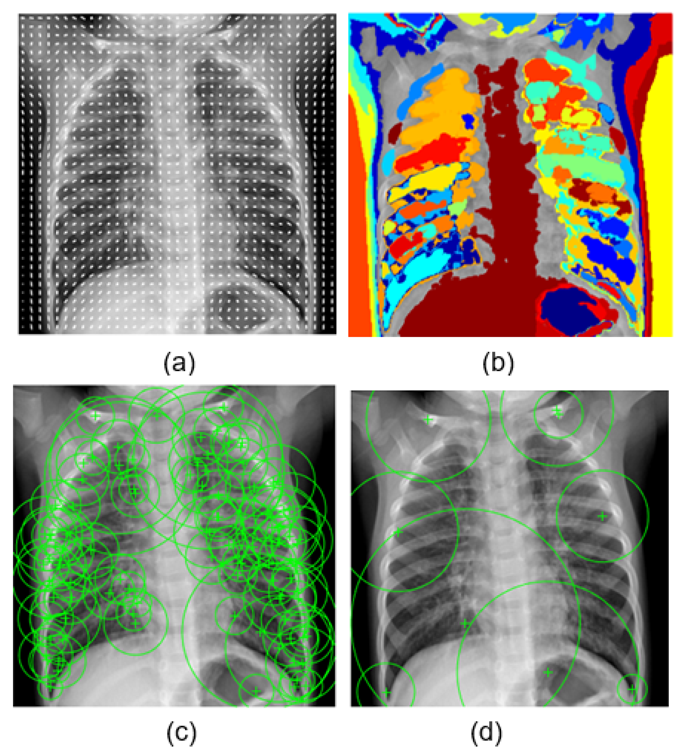
- HOG: Histogram of gradient feature, a grid of equally spaced region plots, is used to show HOG features [45]. The grid dimensions are determined by the image size as well as the cell size. The distribution of gradient orientations within an HOG cell is displayed on each region plot. The region used was a block of cell. The learning was performed by using the strongest 17,693 features from each of the image classes.
- MSER: Maximally stable extremal region is a feature object detector [46]. The MSER object examines changes in region area between various intensity thresholds. Threshold values are used to maintain the circular regions, where circular regions have low eccentricity. The circular region range was [30 14000], and the value of the threshold was 2. Decreasing the value of the threshold will return more regions. The learning was carried out using the 28,550 strongest features.
- SURF: Speeded up robust feature is a patented local feature detector and descriptor [47]. SURF finds landmarks and describes them using a vector that is somewhat resistant to distortion, rotation, and scaling. For this experiment, we used these parameters: number of octaves = 5, number of intervals = 4, and threshold = 0.0004. The most powerful 22,895 features from each of the image classes were used to perform the learning.
- BRISK: Binary robust invariant scalable keypoint is a scale- and rotation-invariant feature point detection and description tool [48]. We used the following parameters for this experiment: number of corners = 0.1, number of octaves = 4, and intensity difference = 0.2. The 6953 most effective features from each class were used to carry out the learning.
4.2. Experiment 2
4.3. Experiment 3
4.4. Discussion
5. Conclusions and Future Work
- First, we recommend that an application be created to function on mobile phones after it has been designed on a computer.
- Second, we advocate using the program to diagnosis other disorders involving the kidneys, such as kidney cancer, because there are few doctors who specialize in identifying kidney ailments, and doctors’ error rates are high, compared to the machine, which has a 91% accuracy rate.
- Third, experimenting with a variety of networks may lead to more accurate disease diagnosis.
- Fourth, this technique not only assists doctors, caretakers, radiologists, and patients with this disease, but it also provides valuable information to researchers who are diagnosing other diseases in the medical domain.
- Fifth, there is still room for improvement in terms of accuracy by using different preprocessing techniques.
Author Contributions
Funding
Conflicts of Interest
References
- AlZu’bi, S.; Jararweh, Y.; Al-Zoubi, H.; Elbes, M.; Kanan, T.; Gupta, B. Multi-orientation geometric medical volumes segmentation using 3d multiresolution analysis. Multimed. Tools Appl. 2018, 78, 24223–24248. [Google Scholar] [CrossRef]
- AlZu’bi, S.; Al-Qatawneh, S.; Alsmirat, M. Transferable HMM Trained Matrices for Accelerating Statistical Segmentation Time. In Proceedings of the 2018 Fifth International Conference on Social Networks Analysis, Management and Security (SNAMS), Valencia, Spain, 15–18 October 2018; pp. 172–176. [Google Scholar]
- AlZu’bi, S.; Mughaid, A.; Hawashin, B.; Elbes, M.; Kanan, T.; Alrawashdeh, T.; Aqel, D. Reconstructing Big Data Acquired from Radioisotope Distribution in Medical Scanner Detectors. In Proceedings of the 2019 IEEE Jordan International Joint Conference on Electrical Engineering and Information Technology (JEEIT), Amman, Jordan, 9–11 April 2019; pp. 325–329. [Google Scholar]
- AlZu’bi, S.; Aqel, D.; Mughaid, A.; Jararweh, Y. A multi-levels geo-location based crawling method for social media platforms. In Proceedings of the 2019 Sixth International Conference on Social Networks Analysis, Management and Security (SNAMS), Granada, Spain, 22–25 October 2019; pp. 494–498. [Google Scholar]
- Zhao, S.; Lin, Q.; Ran, J.; Musa, S.S.; Yang, G.; Wang, W.; Lou, Y.; Gao, D.; Yang, L.; He, D.; et al. Preliminary estimation of the basic reproduction number of novel coronavirus (2019-nCoV) in China, from 2019 to 2020: A data-driven analysis in the early phase of the outbreak. Int. J. Infect. Dis. 2020, 92, 214–217. [Google Scholar] [CrossRef] [PubMed]
- Elbes, M.; Kanan, T.; Alia, M.; Ziad, M. COVD-19 Detection Platform from X-ray Images using Deep Learning. Int. J. Adv. Soft Compu. Appl. 2022, 14, 1. [Google Scholar] [CrossRef]
- Walsh, S.L.; Humphries, S.M.; Wells, A.U.; Brown, K.K. Imaging research in fibrotic lung disease; applying deep learning to unsolved problems. Lancet Respir. Med. 2020, 8, 1144–1153. [Google Scholar] [CrossRef]
- Mughaid, A.; Obeidat, I.; Hawashin, B.; AlZu’bi, S.; Aqel, D. A smart geo-location job recommender system based on social media posts. In Proceedings of the 2019 Sixth International Conference on Social Networks Analysis, Management and Security (SNAMS), Granada, Spain, 22–25 October 2019; pp. 505–510. [Google Scholar]
- Bharati, S.; Podder, P.; Mondal, M.R.H. Hybrid deep learning for detecting lung diseases from X-ray images. Inform. Med. Unlocked 2020, 20, 100391. [Google Scholar] [CrossRef]
- Kieu, S.T.H.; Bade, A.; Hijazi, M.H.A.; Kolivand, H. A survey of deep learning for lung disease detection on medical images: State-of-the-art, taxonomy, issues and future directions. J. Imaging 2020, 6, 131. [Google Scholar] [CrossRef]
- AlZu’bi, S.; Shehab, M.; Al-Ayyoub, M.; Jararweh, Y.; Gupta, B. Parallel implementation for 3d medical volume fuzzy segmentation. Pattern Recognit. Lett. 2020, 130, 312–318. [Google Scholar] [CrossRef]
- Al-Mnayyis, A.; Alasal, S.A.; Alsmirat, M.; Baker, Q.B.; Alzu’bi, S. Lumbar disk 3D modeling from limited number of MRI axial slices. Int. J. Electr. Comput. Eng. 2020, 10, 4101. [Google Scholar] [CrossRef]
- AlZu’bi, S.; Aqel, D.; Mughaid, A. Recent intelligent approaches for managing and optimizing smart blood donation process. In Proceedings of the 2021 International Conference on Information Technology (ICIT), Amman, Jordan, 14–15 July 2021; pp. 679–684. [Google Scholar]
- Sethi, R.; Mehrotra, M.; Sethi, D. Deep learning based diagnosis recommendation for COVID-19 using chest X-rays images. In Proceedings of the 2020 Second International Conference on Inventive Research in Computing Applications (ICIRCA), Coimbatore, India, 15–17 July 2020; pp. 1–4. [Google Scholar]
- Ibrahim, D.M.; Elshennawy, N.M.; Sarhan, A.M. Deep-chest: Multi-classification deep learning model for diagnosing COVID-19, pneumonia, and lung cancer chest diseases. Comput. Biol. Med. 2021, 132, 104348. [Google Scholar] [CrossRef]
- Al-Zu’bi, S.; Hawashin, B.; Mughaid, A.; Baker, T. Efficient 3D medical image segmentation algorithm over a secured multimedia network. Multimed. Tools Appl. 2021, 80, 16887–16905. [Google Scholar] [CrossRef]
- AlZu’bi, S.; Makki, Q.H.; Ghani, Y.A.; Ali, H. Intelligent Distribution for COVID-19 Vaccine Based on Economical Impacts. In Proceedings of the 2021 International Conference on Information Technology (ICIT), Amman, Jordan, 14–15 July 2021; pp. 968–973. [Google Scholar]
- Liu, Q.; Li, N.; Jia, H.; Qi, Q.; Abualigah, L. Modified remora optimization algorithm for global optimization and multilevel thresholding image segmentation. Mathematics 2022, 10, 1014. [Google Scholar] [CrossRef]
- Yousri, D.; Abd Elaziz, M.; Abualigah, L.; Oliva, D.; Al-Qaness, M.A.; Ewees, A.A. COVID-19 X-ray images classification based on enhanced fractional-order cuckoo search optimizer using heavy-tailed distributions. Appl. Soft Comput. 2021, 101, 107052. [Google Scholar] [CrossRef] [PubMed]
- Daradkeh, M.; Abualigah, L.; Atalla, S.; Mansoor, W. Scientometric Analysis and Classification of Research Using Convolutional Neural Networks: A Case Study in Data Science and Analytics. Electronics 2022, 11, 2066. [Google Scholar] [CrossRef]
- AlShourbaji, I.; Kachare, P.; Zogaan, W.; Muhammad, L.; Abualigah, L. Learning Features Using an optimized Artificial Neural Network for Breast Cancer Diagnosis. SN Comput. Sci. 2022, 3, 229. [Google Scholar] [CrossRef]
- Rahman, T.; Khandakar, A.; Qiblawey, Y.; Tahir, A.; Kiranyaz, S.; Kashem, S.B.A.; Islam, M.T.; Al Maadeed, S.; Zughaier, S.M.; Khan, M.S.; et al. Exploring the effect of image enhancement techniques on COVID-19 detection using chest X-ray images. Comput. Biol. Med. 2021, 132, 104319. [Google Scholar] [CrossRef]
- AlZu’bi, S.; AlQatawneh, S.; ElBes, M.; Alsmirat, M. Transferable HMM probability matrices in multi-orientation geometric medical volumes segmentation. Concurr. Comput. Pract. Exp. 2020, 32, e5214. [Google Scholar] [CrossRef]
- AlZu’bi, S.; Aqel, D.; Lafi, M. An intelligent system for blood donation process optimization-smart techniques for minimizing blood wastages. Clust. Comput. 2022, 25, 3617–3627. [Google Scholar] [CrossRef]
- Hussein, F.; Piccardi, M. V-JAUNE: A framework for joint action recognition and video summarization. ACM Trans. Multimed. Comput. Commun. Appl. (TOMM) 2017, 13, 1–19. [Google Scholar] [CrossRef]
- Hubel, D.H.; Wiesel, T.N. Receptive fields, binocular interaction and functional architecture in the cat’s visual cortex. J. Physiol. 1962, 160, 106. [Google Scholar] [CrossRef]
- Howard, A.G.; Zhu, M.; Chen, B.; Kalenichenko, D.; Wang, W.; Weyand, T.; Andreetto, M.; Adam, H. Mobilenets: Efficient convolutional neural networks for mobile vision applications. arXiv 2017, arXiv:1704.04861. [Google Scholar]
- Xu, L.; Ren, J.S.; Liu, C.; Jia, J. Deep convolutional neural network for image deconvolution. Adv. Neural Inf. Process. Syst. 2014, 27, 1790–1798. [Google Scholar]
- Narin, A.; Kaya, C.; Pamuk, Z. Automatic detection of coronavirus disease (covid-19) using x-ray images and deep convolutional neural networks. Pattern Anal. Appl. 2021, 24, 1207–1220. [Google Scholar] [CrossRef]
- Hall, L.O.; Paul, R.; Goldgof, D.B.; Goldgof, G.M. Finding COVID-19 from chest X-rays using deep learning on a small dataset. arXiv 2020, arXiv:2004.02060. [Google Scholar]
- Sanagavarapu, S.; Sridhar, S.; Gopal, T. COVID-19 identification in CLAHE enhanced CT scans with class imbalance using ensembled resnets. In Proceedings of the 2021 IEEE International IOT, Electronics and Mechatronics Conference (IEMTRONICS), Toronto, ON, Canada, 21–24 April 2021; pp. 1–7. [Google Scholar]
- Rajpurkar, P.; Irvin, J.; Zhu, K.; Yang, B.; Mehta, H.; Duan, T.; Ding, D.; Bagul, A.; Langlotz, C.; Shpanskaya, K.; et al. Chexnet: Radiologist-level pneumonia detection on chest X-rays with deep learning. arXiv 2017, arXiv:1711.05225. [Google Scholar]
- Ardakani, A.A.; Kanafi, A.R.; Acharya, U.R.; Khadem, N.; Mohammadi, A. Application of deep learning technique to manage COVID-19 in routine clinical practice using CT images: Results of 10 convolutional neural networks. Comput. Biol. Med. 2020, 121, 103795. [Google Scholar] [CrossRef]
- Dutta, P.; Roy, T.; Anjum, N. COVID-19 detection using transfer learning with convolutional neural network. In Proceedings of the 2021 2nd International Conference on Robotics, Electrical and Signal Processing Techniques (ICREST), Dhaka, Bangladesh, 5–7 January 2021; pp. 429–432. [Google Scholar]
- Sitaula, C.; Hossain, M.B. Attention-based VGG-16 model for COVID-19 chest X-ray image classification. Appl. Intell. 2021, 51, 2850–2863. [Google Scholar] [CrossRef]
- Banerjee, A.; Kulcsar, K.; Misra, V.; Frieman, M.; Mossman, K. Bats and coronaviruses. Viruses 2019, 11, 41. [Google Scholar] [CrossRef]
- Baker, B.; Gupta, O.; Naik, N.; Raskar, R. Designing neural network architectures using reinforcement learning. arXiv 2016, arXiv:1611.02167. [Google Scholar]
- Shibly, K.H.; Dey, S.K.; Islam, M.T.U.; Rahman, M.M. COVID faster R–CNN: A novel framework to Diagnose Novel Coronavirus Disease (COVID-19) in X-ray images. Inform. Med. Unlocked 2020, 20, 100405. [Google Scholar] [CrossRef]
- Bougourzi, F.; Contino, R.; Distante, C.; Taleb-Ahmed, A. CNR-IEMN: A Deep Learning based approach to recognise COVID-19 from CT-scan. In Proceedings of the ICASSP 2021–2021 IEEE International Conference on Acoustics, Speech and Signal Processing (ICASSP), Toronto, ON, Canada, 6–11 June 2021; pp. 8568–8572. [Google Scholar]
- Seum, A.; Raj, A.H.; Sakib, S.; Hossain, T. A comparative study of cnn transfer learning classification algorithms with segmentation for COVID-19 detection from CT scan images. In Proceedings of the 2020 11th International Conference on Electrical and Computer Engineering (ICECE), Dhaka, Bangladesh, 17–19 December 2020; pp. 234–237. [Google Scholar]
- Bikbov, B.; Purcell, C.A.; Levey, A.S.; Smith, M.; Abdoli, A.; Abebe, M.; Adebayo, O.M.; Afarideh, M.; Agarwal, S.K.; Agudelo-Botero, M.; et al. Global, regional, and national burden of chronic kidney disease, 1990–2017: A systematic analysis for the Global Burden of Disease Study 2017. Lancet 2020, 395, 709–733. [Google Scholar] [CrossRef]
- James, R.M.; Sunyoto, A. Detection of CT-Scan lungs COVID-19 image using convolutional neural network and CLAHE. In Proceedings of the 2020 3rd International Conference on Information and Communications Technology (ICOIACT), Yogyakarta, Indonesia, 24–25 November 2020; pp. 302–307. [Google Scholar]
- Pisano, E.D.; Zong, S.; Hemminger, B.M.; DeLuca, M.; Johnston, R.E.; Muller, K.; Braeuning, M.P.; Pizer, S.M. Contrast limited adaptive histogram equalization image processing to improve the detection of simulated spiculations in dense mammograms. J. Digit. Imaging 1998, 11, 193–200. [Google Scholar] [CrossRef] [PubMed]
- Chowdhury, M.E.; Rahman, T.; Khandakar, A.; Mazhar, R.; Kadir, M.A.; Mahbub, Z.B.; Islam, K.R.; Khan, M.S.; Iqbal, A.; Al Emadi, N.; et al. Can AI help in screening viral and COVID-19 pneumonia? IEEE Access 2020, 8, 132665–132676. [Google Scholar] [CrossRef]
- Dalal, N.; Triggs, B. Histograms of oriented gradients for human detection. In Proceedings of the 2005 IEEE computer society conference on computer vision and pattern recognition (CVPR’05), San Diego, CA, USA, 20–25 June 2005; Volume 1, pp. 886–893. [Google Scholar]
- Nistér, D.; Stewénius, H. Linear time maximally stable extremal regions. In Proceedings of the European Conference on Computer Vision, Marseille, France, 12–18 October 2008; pp. 183–196. [Google Scholar]
- Bay, H.; Tuytelaars, T.; Gool, L.V. Surf: Speeded up robust features. In Proceedings of the European Conference on Computer Vision, Graz, Austria, 7–13 May 2006; pp. 404–417. [Google Scholar]
- Leutenegger, S.; Chli, M.; Siegwart, R.Y. BRISK: Binary robust invariant scalable keypoints. In Proceedings of the 2011 International Conference on Computer Vision, Washington, DC, USA, 6–13 November 2011; pp. 2548–2555. [Google Scholar]
- Simonyan, K.; Zisserman, A. Very deep convolutional networks for large-scale image recognition. arXiv 2014, arXiv:1409.1556. [Google Scholar]
- Xue, S.; Abhayaratne, C. COVID-19 diagnostic using 3d deep transfer learning for classification of volumetric computerised tomography chest scans. In Proceedings of the ICASSP 2021–2021 IEEE International Conference on Acoustics, Speech and Signal Processing (ICASSP), Toronto, ON, Canada, 6–11 June 2021; pp. 8573–8577. [Google Scholar]
- Brunese, L.; Martinelli, F.; Mercaldo, F.; Santone, A. Machine learning for coronavirus COVID-19 detection from chest X-rays. Procedia Comput. Sci. 2020, 176, 2212–2221. [Google Scholar] [CrossRef]


| SVM | Accuracy | Classes |
|---|---|---|
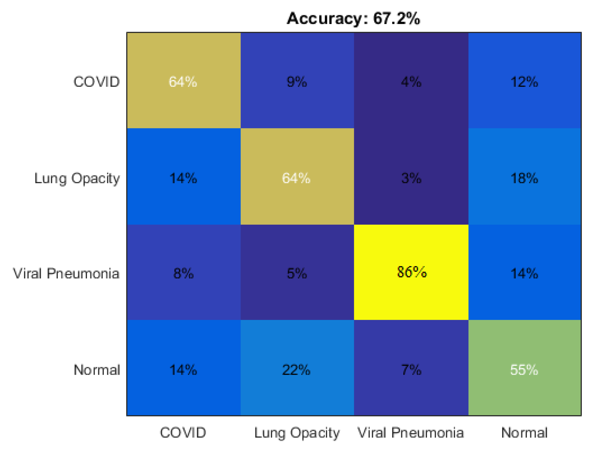
| SVM without using the histogram equalizer | 0.65 | COVID-19 |
| SVM without using the histogram equalizer | 0.64 | Lung opacity |
| SVM without using the histogram equalizer | 0.87 | Viral pneumonia |
| SVM without using the histogram equalizer | 0.56 | NORMAL |
| SVM with the histogram equalizer | 0.64 | COVID-19 |
| SVM with the histogram equalizer | 0.64 | Lung opacity |
| SVM with the histogram equalizer | 0.86 | Viral pneumonia |
| SVM with the histogram equalizer | 0.55 | NORMAL |
| SVM | Accuracy | Precision | Recall | F1 Score |
|---|---|---|---|---|
| HOG without using the histogram equalizer | 0.6891 | 0.6900 | 0.6891 | 2.7563 |
| MSER without using the histogram equalizer | 0.6870 | 0.6868 | 0.6870 | 2.7481 |
| SURF without using the histogram equalizer | 0.6984 | 0.7006 | 0.6984 | 2.7937 |
| BRISK without using the histogram equalizer | 0.6313 | 0.6411 | 0.6313 | 2.5251 |
| HOG with the histogram equalizer | 0.5286 | 0.5173 | 0.5286 | 2.1143 |
| MSER with the histogram equalizer | 0.4643 | 0.4776 | 0.4643 | 1.8571 |
| SURF with the histogram equalizer | 0.6719 | 0.6345 | 0.6714 | 2.9857 |
| BRISK with the histogram equalizer | 0.3500 | 0.3328 | 0.3500 | 1.4000 |
| VGG 19 | Accuracy | Classes | Precision | Recall | F1 Score |
|---|---|---|---|---|---|
| VGG 19 without using the histogram equalizer | 0.70 | COVID-19 | 0.70 | 0.69 | 2.76 |
| VGG 19 without using the histogram equalizer | 0.75 | NORMAL | 0.74 | 0.73 | 2.96 |
| VGG 19 without using the histogram equalizer | 0.76 | Viral pneumonia | 0.76 | 0.75 | 3.00 |
| VGG 19 without using the histogram equalizer | 0.81 | Lung opacity | 0.81 | 0.80 | 3.20 |
| VGG 19 with the histogram equalizer | 0.79 | COVID-19 | 0.79 | 0.77 | 3.12 |
| VGG 19 with the histogram equalizer | 0.82 | NORMAL | 0.82 | 0.80 | 3.24 |
| VGG 19 with the histogram equalizer | 0.85 | Viral pneumonia | 0.85 | 0.84 | 3.36 |
| VGG 19 with the histogram equalizer | 0.88 | Lung opacity | 0.88 | 0.86 | 3.48 |
| CNN | Accuracy | Classes | Precision | Recall | F1 Score |
|---|---|---|---|---|---|
| CNN without using the histogram equalizer | 0.89 | COVID-19 | 0.89 | 0.90 | 3.52 |
| CNN without using the histogram equalizer | 0.86 | NORMAL | 0.86 | 0.85 | 3.40 |
| CNN without using the histogram equalizer | 0.90 | Viral pneumonia | 0.90 | 0.88 | 3.56 |
| CNN without using the histogram equalizer | 0.89 | Lung opacity | 0.89 | 0.87 | 3.52 |
| CNN with the histogram equalizer | 0.89 | COVID-19 | 0.89 | 0.90 | 3.52 |
| CNN with the histogram equalizer | 0.92 | NORMAL | 0.92 | 0.91 | 3.64 |
| CNN with the histogram equalizer | 0.91 | Viral pneumonia | 0.91 | 0.90 | 3.60 |
| CNN with the histogram equalizer | 0.90 | Lung opacity | 0.90 | 0.88 | 3.56 |
| References | Machine Learning Techniques | Accuracy |
|---|---|---|
| [31] | CLAHE, Resnet CNN | 0.87 |
| [34] | CNN | 0.84 |
| [50] | ResNet50 CNN | 0.86 |
| [39] | CNN, ResneXt-50 | 0.87 |
| [40] | VGG19 | 0.89 |
| [42] | CLAHE, CNN | 0.83 |
| [51] | KNN | 0.68 |
| Proposed model | CLAHE, CNN | 0.91 |
| Network | Accuracy |
|---|---|
| SVM without using the histogram equalizer | 0.68 |
| SVM with the histogram equalizer | 0.67 |
| VGG 19 without using the histogram equalizer | 0.76 |
| VGG 19 with the histogram equalizer | 0.84 |
| CNN without using the histogram equalizer | 0.89 |
| CNN with the histogram equalizer | 0.91 |
Publisher’s Note: MDPI stays neutral with regard to jurisdictional claims in published maps and institutional affiliations. |
© 2022 by the authors. Licensee MDPI, Basel, Switzerland. This article is an open access article distributed under the terms and conditions of the Creative Commons Attribution (CC BY) license (https://creativecommons.org/licenses/by/4.0/).
Share and Cite
Hussein, F.; Mughaid, A.; AlZu’bi, S.; El-Salhi, S.M.; Abuhaija, B.; Abualigah, L.; Gandomi, A.H. Hybrid CLAHE-CNN Deep Neural Networks for Classifying Lung Diseases from X-ray Acquisitions. Electronics 2022, 11, 3075. https://doi.org/10.3390/electronics11193075
Hussein F, Mughaid A, AlZu’bi S, El-Salhi SM, Abuhaija B, Abualigah L, Gandomi AH. Hybrid CLAHE-CNN Deep Neural Networks for Classifying Lung Diseases from X-ray Acquisitions. Electronics. 2022; 11(19):3075. https://doi.org/10.3390/electronics11193075
Chicago/Turabian StyleHussein, Fairouz, Ala Mughaid, Shadi AlZu’bi, Subhieh M. El-Salhi, Belal Abuhaija, Laith Abualigah, and Amir H. Gandomi. 2022. "Hybrid CLAHE-CNN Deep Neural Networks for Classifying Lung Diseases from X-ray Acquisitions" Electronics 11, no. 19: 3075. https://doi.org/10.3390/electronics11193075
APA StyleHussein, F., Mughaid, A., AlZu’bi, S., El-Salhi, S. M., Abuhaija, B., Abualigah, L., & Gandomi, A. H. (2022). Hybrid CLAHE-CNN Deep Neural Networks for Classifying Lung Diseases from X-ray Acquisitions. Electronics, 11(19), 3075. https://doi.org/10.3390/electronics11193075