Abstract
For the problem of overhead line broken strand identification, a VMD−SSA−SVM-based overhead transmission line broken strand identification method is proposed. First, the vibration acceleration response signal of overhead transmission line under breeze environment was simulated by Ansys simulation software. Then the variable modal decomposition of the vibration acceleration response of the transmission line is performed to obtain the intrinsic mode function corresponding to the vibration behavior of the transmission line. The Hilbert transform is used to analyze the intrinsic mode functions of each order, and the Hilbert spectrum and marginal spectrum of the intrinsic mode functions of each order are studied to extract the first six order intrinsic frequencies. Each set of intrinsic frequencies is input as a feature vector into a support vector machine optimized by the sparrow search algorithm for training to achieve the identification of broken strands in overhead transmission lines. This paper studies the inherent frequency changes and identification results of overhead transmission lines under two states of normal operation and broken 5 strands operation, and the test results show that the identification method based on VMD-SSA-SVM has good identification effect on broken strands of overhead lines.
1. Introduction
Overhead transmission lines are an important part of the power system and are the main carrier for power transmission and distribution. Transmission lines work in harsh environments, are exposed to wind and sun for long periods of time and can withstand lightning strikes in extreme weather conditions, even in freezing conditions. The transmission lines of the broken shares and the wear of the situation are very easily caused. This affects the safe operation of the transmission line. If the transmission line is not found in time and repaired, it will seriously affect residents’ electricity consumption and industrial production, and cause serious economic loss. In order to ensure the normal operation of transmission lines, it is of great significance to detect broken strands and damage to transmission lines in real time [1,2].
The current overhead transmission line broken strand detection mainly uses three methods: the first is based on the damage detection theory of transmission line broken strand identification method, mainly including electromagnetic induction method [3], eddy current detection method [4], ultrasonic detection method [5]. These three damage detection methods can well solve the effects of the electric characteristics of natural environment and overhead transmission lines, but to realize accurate identification, it is necessary to match the position of the sensor with that of the circuit breakers. The second is a broken strand identification method based on image recognition theory, which is carried out by means of an image acquisition system combined with an intelligent algorithm to extract the outline of the broken strand or damage location of the transmission line [6,7,8]. This method can observe transmission line disconnection more intuitively, but when there is dirt on the surface of transmission line surface, it has a certain effect on the recognition effect. Most of the above two methods need to work with patrol robots or drones. The third method is to predict the fatigue life of transmission line during operation based on the stress analysis of transmission line stress, and to establish a life prediction model in order to maintain or replace the remaining transmission line as soon as possible [9,10]. However, the accuracy of life prediction models often does not meet the needs of actual engineering. The advantages and disadvantages of each approach are compared in Table 1.

Table 1.
Comparison of identification methods of overhead transmission lines.
Overhead transmission lines are structurally a mechanical structure made of steel or aluminum stranded wires stranded concentrically. In the related mechanical structure diagnosis problem, the fault diagnosis method of using the measured vibration signal to extract the intrinsic frequency of overhead transmission lines and then analyzing the intrinsic frequency to determine the fault has been widely used [11,12,13]. Similarly, the vibration signal of the overhead line in the breeze environment contains rich state information, and its vibration characteristics change when the wire is broken, mainly in the change of its intrinsic frequency. On the basis of this, it is a powerful criterion to judge the normal operation state of overhead transmission line by extracting the inherent frequency characteristics and analyzing the change law of the breeze vibration signal. Ref [14] used the random subspace identification method(RSM) to extract the intrinsic frequency information in transmission line vibration signals and achieved good experimental results. However, the RSM method is slow, time-consuming, and requires high hardware requirements. The variational modal decomposition method(VMD) is a new adaptive modal parameter extraction method proposed by Dragomiretskiy and Zosso in 2014, which has the characteristics of fast convergence and obvious decomposition results [15]. At present, the VMD method is mostly applied to the fault diagnosis of rotating machinery structures, ref [16] took the combination of VMD method and energy entropy for the vibration signal feature extraction of wind turbines, in addition to doing a comparison with empirical mode decomposition (EMD) method, and the results show that the accuracy of VMD method is higher than EMD method. Moreover, VMD is widely used to remove the noise from the signal [17,18]. In addition, in order to meet the needs of intelligent development of power grid, a machine learning algorithm proposed to realize the identification of transmission lines disconnection. Support vector machines(SVM) are commonly used to solve linear/nonlinear and high-dimensional problems [19], and they are susceptible to penalty parameters and kernel functions when dealing with classification problems. Therefore, it needs to be optimized in practical engineering applications, usually using genetic algorithm(GA) [20] and particle swarm algorithm(PSO) [21]. The GA algorithm is slow in search speed when training, so it needs more training time. In PSO algorithm, although the search speed is fast, it is easy to fall into the local optimal solution so the accuracy rate is low. In addition, the sparrow search algorithm(SSA) has been widely used since its proposal; it is combined with support vector machines in classification problems [22,23]. This paper also compares the recognition effects of the above three methods in the identification of broken strands in overhead transmission lines.
Aiming at the requirement of transmission line breakage identification, this paper first models and simulates the transmission line before and after the breakage, and analyzes the acceleration response signal according to the vibration state of breeze. VMD−SSA−SVM identification model is used to identify broken strands in overhead transmission lines. The VMD method is used to decompose the acceleration response signals under different broken strands of transmission lines, and then the decomposed intrinsic mode functions are subjected to Hilbert−Huang transform (HHT), combined with the joint analysis method of Hilbert spectrum and marginal spectrum, the first six orders of intrinsic frequencies of broken strands of transmission lines are screened out, and each set of intrinsic frequencies is input as an input vector into SSA−SVM classifier to classify the broken and normal states in order to achieve the broken strand identification of transmission lines.
2. Principle Related to Overhead Line Broken Strand Identification Model
2.1. Variational Modal Decomposition (VMD)
With the signal , the VMD decomposition decomposes into multiple intrinsic mode function (IMF) components, each mode has its central frequency . On this basis, it is also necessary to solve the constrained variational model to determine the bandwidth of each IMF, so the following model needs to be solved.
In the above Equation (1): denotes the intrinsic modal components obtained by decomposition; denotes the central frequency of each modal component; where . is the unit pulse function, is an imaginary unit, is the convolution operation, is the partial derivative of the function for time, is the objective function.
By introducing a quadratic penalty factor and a Lagrangian operator , the above equation is transformed into an unconstrained variational problem, forming an augmented Lagrangian function whose expression is:
The “saddle point” in Equation (2) is found by the alternating directional multiplier algorithm (ADMM), and a series of and are obtained, which are the center frequencies and bandwidths of the K modal components. The specific solution steps are shown in Appendix A.
2.2. Hilbert−Huang Transform−Marginal Spektrum
The individual IMFs after the variational modal decomposition are the original signal components of a single group, and the Hilbert transform is applied to separately.
where denotes the time series of each modal component; denotes the analytic signal of the corresponding modal component. The complex and polar forms of the constructed analytic function are expressed as:
In Equation (4), denotes the instantaneous amplitude of each mode component and denotes the instantaneous phase of each mode component. The relationship between amplitude, phase and frequency is shown in Appendix A.
The Hilbert spectrum is used to represent the relationship between time, frequency, and amplitude, and the Hilbert marginal spectrum is obtained by integrating in time.
2.3. Sparrow Search Algorithm (SSA)
The sparrow search algorithm is an intelligent optimization algorithm that was created by the nature sparrow’s habit of feeding, following, and scouting. The sparrow species are divided into two categories: discoverers find the best foraging position, while the followers search around the discoverers and compete for the best foraging position, and when the followers find a better foraging position they update the discoverers’ foraging position. Once foraging is threatened, the marginal sparrow will give a warning and return to the safety zone, and the best foraging location sparrows move in the nearby location. The optimal solution in the algorithm corresponds to the foraging position of the discoverer, and the discoverer continuously updates the foraging position to represent the iterative process in the algorithm. The process is described in detail as follows:
Position update formula for discoverer during iteration:
where, when , it indicates that the environment of the current foraging location is safe and the finder can search in a wide range. Conversely, when , it means that the marginal sparrows have found the danger, and all sparrows need to go to other location models to feed at this time. denotes the position of the sparrow in dimension , denotes the number of iterations; denotes a random number between ; denotes the maximum number of iterations; denotes the warning value takes a range of ; denotes the safety value takes a range of ; is a normally distributed random number; and denotes a matrix with elements of 1.
Follower’s position update formula:
where denotes the worst position; denotes the follower with a low adaptation degree does not obtain food and needs to fly to other positions to feed; denotes the optimal position; , denotes a matrix with elements randomly assigned to 1 or −1.
When faced with danger, a portion of the sparrows send out warning messages, and their locations are updated with the following formula:
where, when , it means that the sparrow is at the edge of the population and is vulnerable to danger. is the current global optimal foraging position, and is a normally distributed random number with mean 0 and variance 1 for step control. When , it means that the sparrow in the middle of the population receives danger information and needs to move to the position of other sparrows to reduce the risk of predation. is a random number of . is the current individual sparrow fitness value, and are the current global best and worst fitness values, respectively, and is a constant used to avoid a denominator of 0.
2.4. Support Vector Machine Classification Principle (SVM)
Support vector machine is a machine learning method. In performing classification, it is the transformation of linearly indistinguishable samples in a low−dimensional space into linearly distinguishable samples in a high-dimensional space by transforming the high-dimensional space, and the goal is to find the optimal classification hyperplane that maps to the high−dimensional space. The mathematical description is as follows:
where is the bias vector. is the weight vector. is the penalty parameter that controls the degree of penalty for misclassified samples. is the relaxation variable, indicating the degree of misclassification of the training samples. By introducing Lagrange multipliers, it is transformed into a pairwise quadratic programming problem, which leads to the optimal classification decision function:
For nonlinear classification problems, it is usually necessary to introduce a kernel function mapping to find the optimal classification surface in a high−dimensional space, and the optimal classification decision function obtained after introducing the kernel function is:
In Equation (10), are the solutions of the functions, which denote the weights corresponding to the SVM optimized samples and the threshold of the optimized SVM classifier, respectively, is the number of training samples, and is the desired output; is the input vector. The kernel function chosen in this paper is Gaussian Kernel:
It is easy to see from the above assortment that the main parameters affecting the classification performance of SVM are the penalty function and the kernel function . In this regard, the optimization of SVM parameters using SSA is proposed to improve the classification effect of SVM.
3. VMD−SSA−SVM Identification Model
Coupling VMD, SSA, and SVM into a VMD−SSA−SVM discriminative model. The VMD method decomposes the measured overhead line vibration signal into components, and selects the appropriate components to reconstruct the signal to realize the noise reduction process of the original signal. After that, a second VMD decomposition is performed on the reconstructed signal, and the HHT transform is applied to each component of the decomposition to obtain the corresponding marginal spectrum to extract the vibration features as the input to the SSA−SVM classifier. Second, the parameters of SSA, such as sparrow population size , maximum number of iterations , and parameter range, need to be set, and the penalty parameter and kernel parameter of SVM are optimized to finally realize the identification of overhead line broken strands under vibration state. The VMD−SSA−SVM identification model is shown in Figure 1.
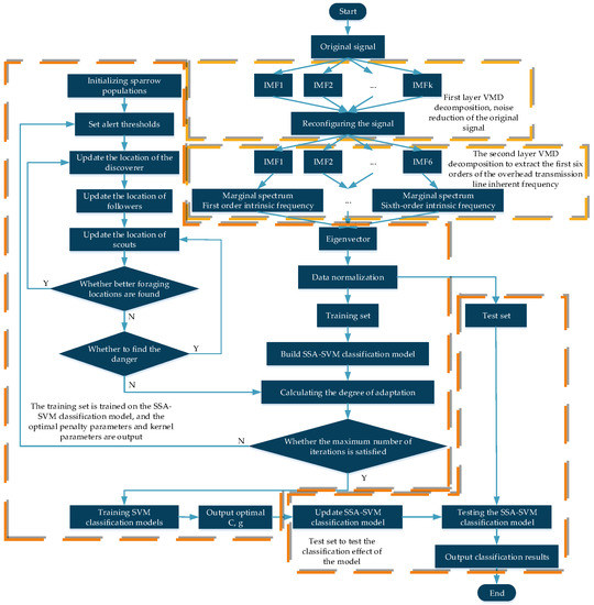
Figure 1.
Basic flow of VMD-SSA-SVM identification model.
The main steps of the model are as follows:
Step 1: Generate overhead transmission line vibration signals using simulation software.
Step 2: The original signal is decomposed by VMD, the correlation coefficient threshold is set, the IMF component is selected for signal reconstruction, and the noise reduction process of the original signal is realized.
Step 3: VMD decomposition is performed on the reconstructed signal; the marginal spectrum of each IMF component is obtained by HHT transformation of the last six orders of IMF components, and the eigenfrequencies of the first six orders of the overhead transmission line are extracted.
Step 4: Initialize the SSA−SVM classifier parameters.
Step 5: The extracted first six orders of intrinsic frequencies are input as feature vectors and trained for classification.
Step 6: Start iterating to calculate the fitness value of each sparrow and update the positions of discoverer, follower, and scout.
Step 7: Determine whether it is the optimal solution, if so, output the optimal solution, otherwise return to step 6 and continue iteration.
Step 8: Enter the test set for testing to determine whether the overhead transmission line is broken in the vibration condition.
Overall, the model uses a combination of two layers of VMD decomposition and an SSA-optimized SVM classifier. Through the first layer of VMD VMD decomposition the original signal is noise reduction, the high frequency noise of jamming signal feature extraction is eliminated, and the spatial complexity of subsequent signal feature extraction is reduced. The second layer of VMD decomposition uses the spectral analysis method to extract the first six orders of the overhead transmission line’s intrinsic frequency results, which are more accurate and intuitive. SSA−optimized SVM classifier uses global search penalty parameters and kernel functions to find the optimal SVM classifier, which reduces the time complexity of the algorithm compared with other optimization methods. The experimental results show that this method is optimal under the condition of classification accuracy and running time metrics.
4. Dynamics Simulation of Overhead Transmission Lines
Overhead lines are usually formed by concentric twisting of steel and aluminum wires, but can be approximated as a cylinder under macroscopic conditions. In the breezy environment, Kalman vortex will cause the transmission line in the vertical direction to produce up and down alternating forces, thus resulting in the transmission line in the vertical direction of vibration [24]. As shown in Figure 2.
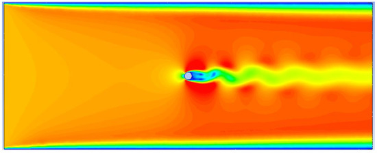
Figure 2.
Kalman vortex.
The overhead transmission line model shown in Figure 3 is established using Ansys software, set to be 5 m long, 0.0108 m radius, with a modulus of elasticity of 70,500 MPa, density of 2524.3 kg/m3, and Poisson’s ratio of 0.3. The boundary conditions under static conditions are: A for natural gravity, B end to release the degrees of freedom in the X direction, C for a tension load of 12,000 N, and D end for fixed constraints.
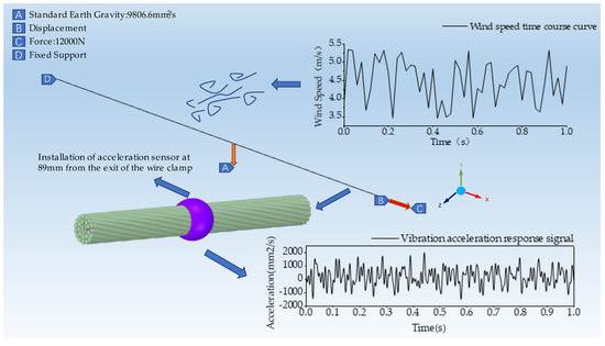
Figure 3.
Simulation system model.
In order to simulate the breeze vibration generated by the overhead transmission line in a breezy environment, it is necessary to simulate the breeze speed time curve, based on the “Beaufort scale” breeze wind speed of 3.4 m/s~5.4 m/s. The simulated wind speed time profiles are shown in Figure 3. In this paper, it is assumed that the wind load acts vertically with the transmission line along the Z−axis direction. Then use Ansys to carry out transient dynamics analysis on the model in the figure, transient dynamics analysis is to reflect the structural dynamic response of the structure under the action of time-varying load, set the analysis time to 1 s, and get the vibration acceleration response of the overhead transmission line as shown in Figure 3.
5. Results and Analysis
In the actual operation of transmission lines, there are often interference signals such as electromagnetic interference, so random noise is superimposed on the vibration signal obtained from the simulation to more closely match the actual vibration response signal obtained. This paper simulates two overhead line operation states with and without broken strands and broken 5 strand transmission lines. The time domain waveforms of the original vibration signal and the superimposed random noise under normal operation are shown in Figure 4.
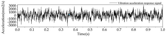
Figure 4.
Vibration signal after superimposing random noise in normal condition.
5.1. VMD Decomposition Spurious Component Determination and Signal Reconstruction
Under normal operation condition, the vibration response signals is decomposed by VMD and the number of decomposing layers is 6. The decomposition results are shown in Figure 5, respectively. IMFi denotes the ith intrinsic mode function component of the decomposition. The center frequencies of each component and the correlation coefficients between each component and the original signal are shown in Figure 6.
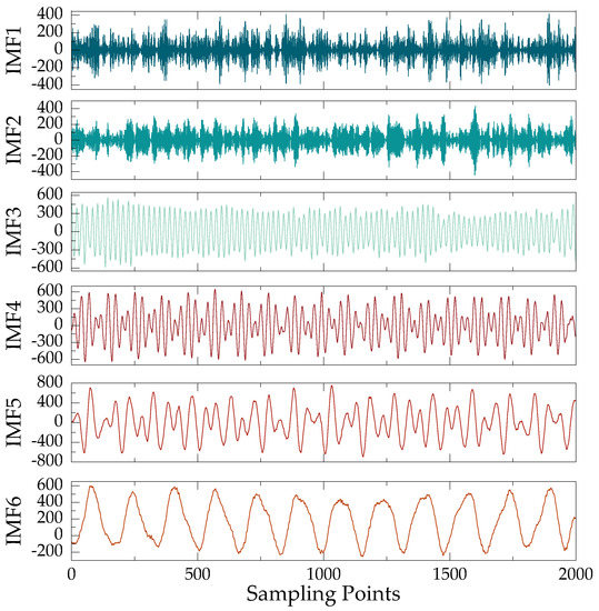
Figure 5.
Results of the first layer VMD decomposition of vibration signal under normal operation.
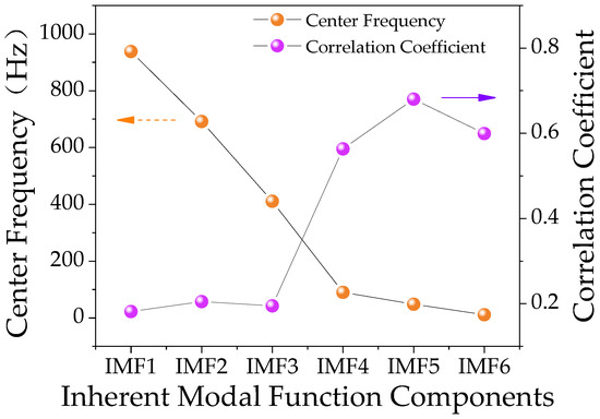
Figure 6.
The first layer VMD decomposes the correlation coefficient of each IMF component with the signal superimposed noise and the center frequency of each mode.
From the decomposition results, it can be seen that IMF1~IMF3 show high noise components because of the noise, and their characteristics are close to the noise characteristics, while IMF4~IMF6 contain the main information of overhead line vibration. The individual IMF components from the VMD decomposition results can only be used to initially determine the IMF components for the next signal reconstruction.
When selecting IMF component reconstruction signal, combining the center frequency of each component and its self-correlation coefficient with the correlation coefficient of the original signal to filter the IMF component, we can effectively distinguish the real IMF component from the noise component, and retain the real IMF component for signal reconstruction, so as to achieve noise reduction.
According to Figure 7, it is easy to see that the center frequencies of IMF1~IMF3 are significantly larger than IMF4~IMF6. The vibration frequency of the overhead line in the actual statistical results is less than 100 Hz [25], and the decomposition results show that the vibration information of the overhead line below 100 Hz is mainly contained in IMF4~IMF6; and the correlation between IMF4~IMF6 and the original signal is higher than IMF1 ~IMF3 are higher than 0.5, so IMF4~IMF6 are selected as the reconstructed signals for VMD decomposition.
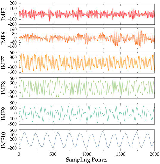
Figure 7.
Post-sixth order intrinsic mode function components of the VMD decomposition results of the reconstructed signal.
5.2. VMD Decomposition of Reconstructed Signals with HHT Transform
The reconstructed signal is then decomposed by VMD, and in this paper, the method of observing the center frequency is used to determine the number of modes for the decomposition [26], and the center frequencies of different modal numbers are shown in Table 2.
Table 2.
Center frequencies corresponding to different modal numbers.
From Table 2, it can be seen that when the number of modes is 10, the center frequency of the last six orders of modes basically no longer changes, and when the number of modes is 11, IMF6 and IMF7 have similar center frequencies, and there is an over−decomposition situation. Therefore, the number of modal decomposition layers is 10, and the results of the decomposition of the last six orders are shown in Figure 7, and the corresponding Hilbert spectra of the IMF components of the last six orders are shown in Figure 8.
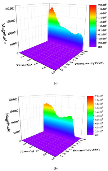
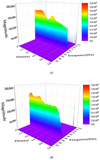
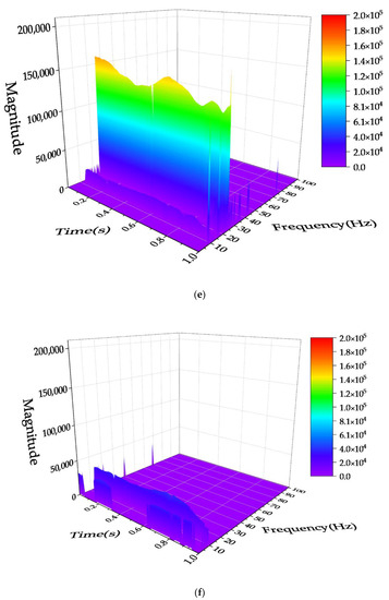
Figure 8.
Hilbert spectra of IMF5~IMF10; where, Figs. a~f are Hilbert spectra corresponding to IMF5~IMF10, respectively. (a) IMF5 Hilbert Spectrum. (b) IMF6 Hilbert Spectrum. (c) IMF7 Hilbert Spectrum. (d) IMF8 Hilbert Spectrum. (e) IMF9 Hilbert Spectrum. (f) IMF10 Hilbert Spectrum.
From Figure 8a, it can be seen that the energy features contained in IMF5 are mainly concentrated around 100 Hz. Figure 8b shows that the energy features contained in IMF6 are stable between 70 and 80 Hz. Figure 8c shows that the energy features contained in IMF7 are stable between 50 and 60 Hz. Figure 8d shows that the energy features contained in IMF8 are concentrated around 40 Hz. Figure 8e shows that the energy features contained in IMF9 is mainly concentrated between 20 and 30 Hz, but there is a weaker energy feature between 10 and 20 Hz. Figure 8f shows that the energy feature contained in IMF10 is mainly concentrated between 10 and 20 Hz, which is probably the same as the fainter energy signature shown in Figure 8e. From the above results, it can be seen that the intrinsic frequencies of overhead transmission conductors within 100 Hz are shown near 10 Hz, 25 Hz, 40 Hz, 50 Hz, 75 Hz, and 100 Hz.
In order to extract the inherent frequency of the overhead line more accurately, the above Hilbert spectrum is used for time integration, and the frequency-time-energy relation is converted into a frequency-amplitude relationship. The marginal spectrum of each IMF is obtained to reflect the frequency of the vibration response signal more accurately. The marginal spectrum obtained by each IMF is shown in Figure 9.
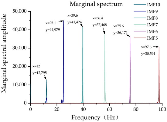
Figure 9.
Marginal spectrum of IMF5~IMF10.
The results of the VMD−HHT method to obtain the intrinsic frequencies of the overhead line in the operation state without broken strands and with 5 broken strands with Ansys modal analysis are shown in Table 3.
Table 3.
Comparison of inherent frequency results obtained from VMD method and FEM simulation modal analysis.
As can be seen from the table, the first six orders of inherent frequencies obtained by the identification method based on VMD−HHT are close to the results obtained by Ansys software and have a high practical utilization value. The self−oscillation frequencies identified under the operating conditions of no broken strands and broken 5 strands have a significant decrease above the 3rd order, which has a good identification effect on the broken strands of overhead lines.
5.3. VMD-SSA-SVM Model Identification Results
According to the self-oscillation frequencies of wires in normal operation state and broken 5−strand operation state extracted by VMD method, 150 samples are taken from each group, 300 samples in total. Assign the classification label to 1 for the normal operation status and 2 for the broken 5−strand operation transition counter. Each group of 75 samples is used as the training set to train the model, and the remaining group of 75 samples is used as the test set to test the model, with the recognition index of accuracy. The penalty parameter C and the kernel function g are two important parameters in the support vector machine, which affect the accuracy of the classification model. Therefore, selecting the optimal C and g is the key to SVM optimization, which is the purpose of this paper to propose the optimization of SVM with SSA algorithm. After repeated experiments, the parameters of the SSA algorithm were finally determined in this paper as follows: the number of sparrows N = 20, the maximum number of iterations Tmax = 100; the penalty parameter C = 970.593 and g = 31.833 for the SVM after optimization by SSA. In order to examine the classification effect of SSA−SVM models, SVM models optimized by genetic algorithm (GA) and particle swarm algorithm (PSO) are selected for comparison. The penalty parameter C = 688.015, g = 31.738 for GA−SVM optimization and C = 24.581, g = 2.398 for PSO−SVM optimization. The resulting classification results are shown in Figure 10, Figure 11 and Figure 12.
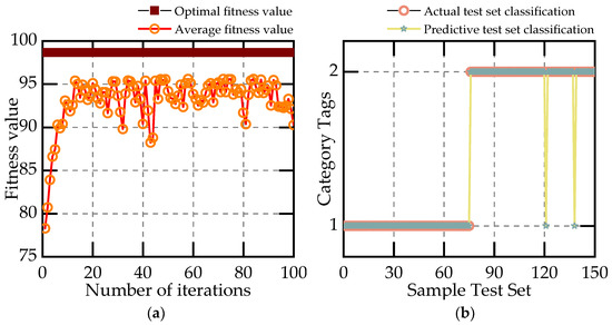
Figure 10.
Classification graph of GA-SVM classifier. (a) Adaptability curve. (b) Classification chart.
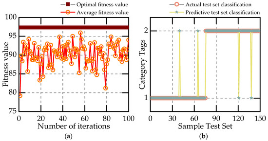
Figure 11.
Classification graph of PSO-SVM classifier. (a) Adaptability curve. (b) Classification chart.
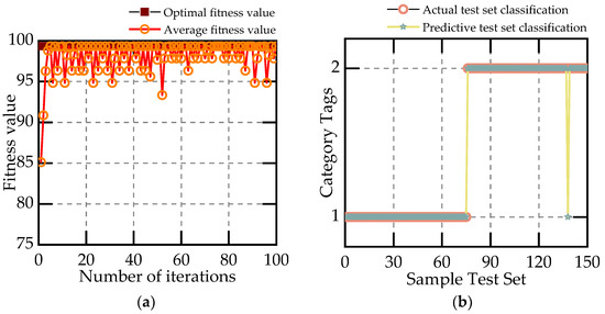
Figure 12.
Classification graph of SSA-SVM classifier. (a) Adaptability curve. (b) Classification chart.
As can be seen from the figure, the distance between the average fitness value and the optimal fitness value of the PSO optimization algorithm is too large, which leads to poor fitting and reduced classification accuracy. The GA optimization algorithm outperforms the PSO algorithm in this respect, but is worse than the SSA algorithm. Among the test results of the three algorithms, SSA−SVM has the highest accuracy and PSO−SVM has the lowest accuracy. Table 4 shows the accuracy and running time of each algorithm.
Table 4.
Classification accuracy and running time of classification models.
By comparing the three recognition algorithms, it is found that the SSA−SVM model has better performance and stability than the others. In terms of run time, PSO−SVM has the shortest run time, but the lowest accuracy, and GA−SVM has the longest run time. Overall, the SSA-SVM has the best overall performance.
6. Conclusions
In this paper, overhead lines are simulated under breeze vibration using Ansys finite element analysis software, and the vibration acceleration response signals of transmission lines are obtained. A two−layer VMD coupled with SSA−SVM is proposed to reduce the noise of the original signal and extract the first six orders of intrinsic frequencies of the overhead transmission line, and then each set of extracted intrinsic frequencies is input into the SSA−SVM classification model as a feature vector to achieve the identification of broken strands of the overhead transmission line; in this paper, two operating states of the overhead line, normal operation and broken 5 strands, are tested in different identification. In this paper, it is found that there is a significant decrease in the intrinsic frequency of the conductor above the third order after the broken strand, and the best effect of SSA−SVM for this recognition is compared with three support vector machine classification methods.
Although the experimental results are good, the increased noise is Gaussian white noise, which cannot accurately reflect the actual work environment noise, which has some limitations. In the next work, a vibration acquisition device will be designed to analyze the noise and improve the algorithm by collecting the response signals of the working environment of the actual overhead transmission line.
Author Contributions
Conceptualization, C.W.; methodology, C.W.; software, C.W.; validation, C.W.; formal analysis, C.W.; investigation, C.W. and S.W.; resources, H.L. and J.Z.; data curation, J.L. and J.W.; writing—original draft preparation, C.W.; writing—review and editing, C.W.; visualization, C.W.; supervision, H.L.; project administration, H.L.; funding acquisition, H.L. and J.Z. All authors have read and agreed to the published version of the manuscript.
Funding
The study was funded by the Enshi Power Supply Company of State Grid Hubei Electric Power Ltd. (B715P022004W).
Data Availability Statement
Not applicable.
Conflicts of Interest
The author declares no conflict of interest.
Appendix A
The specific steps for solving Equation (2) by the alternating direction multiplier algorithm in Section 2.1 are as follows:
- (1)
- Initialize , and let ;
- (2)
- Iteratively update , and :
In Equations (A4)–(A6), the parameter is the fidelity coefficient, which is used to meet the fidelity requirement of signal decomposition. , , , and are the forms of , , , and after Fourier transform, respectively.
- (3)
- The size of the judgment accuracy in Equation (6) is used to decide whether the iteration is stopped or not, so that the optimal each mode component and the central frequency are derived.
- (4)
- Outputs the K modal components and its corresponding center frequency values.
The expressions of amplitude, phase, and frequency of each modal component of the analytic function constructed in Section 2.2 are as follows:
The instantaneous amplitude of each modal component is expressed as:
The instantaneous phase of each modal component is expressed as:
The derivative of the instantaneous phase is the instantaneous frequency of the corresponding modal component:
References
- Shi, L.; Yang, H.; Xu, L.; Yang, Y.; Wang, D.; Long, X.; Zhao, J. Fast detection method of transmission line defects and faults based on airborne laser LiDAR. J. Physics Conf. Ser. 2021, 2005, 12240. [Google Scholar]
- Ma, X.; Gao, L.; Zhang, J.; Zhang, L.-C. Fretting Wear Behaviors of Aluminum Cable Steel Reinforced (ACSR) Conductors in High-Voltage Transmission Line. Metals 2017, 7, 373. [Google Scholar] [CrossRef]
- Miu, Z.; Wu, N.; Yao, J.; Ke, X.; Liu, P.; Bie, S. Fault Diagnosis of Transmission Lines Based on High Frequency Electromagnetic Spectrum Distribution Characteristics. J. Phys. Conf. Ser. 2022, 2166, 12017. [Google Scholar] [CrossRef]
- Liao, C.; Yi, Y.; Chen, T.; Cai, C.; Deng, Z.; Song, X.; Lv, C. Detecting Broken Strands in Transmission Lines Based on Pulsed Eddy Current. Metals 2022, 12, 1014. [Google Scholar] [CrossRef]
- Kim, D.; Kim, S.; Jeong, S.; Ham, J.-W.; Son, S.; Oh, K.-Y. Damage Detection with an Ultrasound Array and Deep Convolutional Neural Network Fusion. IEEE Access 2020, 8, 189423–189435. [Google Scholar] [CrossRef]
- Zhang, Y.; Huang, X.; Jia, J.; Liu, X. A Recognition Technology of Transmission Lines Conductor Break and Surface Damage Based on Aerial Image. IEEE Access 2019, 7, 59022–59036. [Google Scholar] [CrossRef]
- Cao, G.; Liu, Y.; Fan, Z.; Chen, L.; Mei, H.; Zhang, S.; Wang, J.; Han, X. Research on Small-scale Defect Identification and Detection of Smart Grid Transmission Lines Based on Image Recognition. In Proceedings of the 2021 IEEE 4th International Conference on Automation, Electronics and Electrical Engineering (AUTEEE), Shenyang, China, 19–21 November 2021; pp. 423–427. [Google Scholar]
- Zhou, Y.; Sun, H.; Liu, C.; Zhang, J.; Zhu, Z.; Tang, B. Automatic Recognition Method of Broken Transmission Line Defect Image Based on Deep Transfer Learning. J. Phys. Conf. Ser. 2022, 2189, 12002. [Google Scholar] [CrossRef]
- Redford, J.; Gueguin, M.; Nguyen, M.; Lieurade, H.-P.; Yang, C.; Hafid, F.; Ghidaglia, J.-M. Calibration of a numerical prediction methodology for fretting-fatigue crack initiation in overhead power lines. Int. J. Fatigue 2019, 124, 400–410. [Google Scholar] [CrossRef]
- Liu, J.; Yan, B.; Mou, Z.; Gao, Y.; Niu, G.; Li, X. Numerical study of aeolian vibration characteristics and fatigue life estimation of transmission conductors. PLoS ONE 2022, 17, e0263163. [Google Scholar] [CrossRef]
- Altunışık, A.C.; Okur, F.Y.; Kahya, V. Modal parameter identification and vibration based damage detection of a multiple cracked cantilever beam. Eng. Fail. Anal. 2017, 79, 154–170. [Google Scholar] [CrossRef]
- Hou, J.; Xu, D.; Jankowski, Ł.; Liu, Y.; Monitoring, H. Constrained mode decomposition method for modal parameter identification. Struct. Control Health Monit. 2022, 29, e2878. [Google Scholar] [CrossRef]
- Wei, B.; Xie, B.; Li, H.; Zhong, Z.; You, Y. An improved Hilbert–Huang transform method for modal parameter identification of a high arch dam. Appl. Math. Model. 2021, 91, 297–310. [Google Scholar] [CrossRef]
- Zhao, L.; Huang, X.; Jia, J.; Zhu, Y.; Cao, W. Detection of Broken Strands of Transmission Line Conductors Using Fiber Bragg Grating Sensors. Sensors 2018, 18, 2397. [Google Scholar] [CrossRef] [PubMed]
- Dragomiretskiy, K.; Zosso, D. Variational mode decomposition. IEEE Trans. Signal Processing 2013, 62, 531–544. [Google Scholar] [CrossRef]
- Chen, X.; Yang, Y.; Cui, Z.; Shen, J. Vibration fault diagnosis of wind turbines based on variational mode decomposition and energy entropy. Energy 2019, 174, 1100–1109. [Google Scholar] [CrossRef]
- Yang, H.; Li, L.-L.; Li, G.-H.; Guan, Q.-R. A novel feature extraction method for ship-radiated noise. Def. Technol. 2022, 18, 604–617. [Google Scholar] [CrossRef]
- Feng, G.; Wei, H.; Qi, T.; Pei, X.; Wang, H. A transient electromagnetic signal denoising method based on an improved variational mode decomposition algorithm. Measurement 2021, 184, 109815. [Google Scholar] [CrossRef]
- Ceperic, E.; Ceperic, V.; Baric, A. A Strategy for Short-Term Load Forecasting by Support Vector Regression Machines. IEEE Trans. Power Syst. 2013, 28, 4356–4364. [Google Scholar] [CrossRef]
- Tang, H.; Yuan, Z.; Dai, H.; Du, Y. Fault Diagnosis of Rolling Bearing Based on Probability box Theory and GA-SVM. IEEE Access 2020, 8, 170872–170882. [Google Scholar] [CrossRef]
- Cuong-Le, T.; Nghia-Nguyen, T.; Khatir, S.; Trong-Nguyen, P.; Mirjalili, S.; Nguyen, K.D. An efficient approach for damage identification based on improved machine learning using PSO-SVM. Eng. Comput. 2021, 38, 3069–3084. [Google Scholar] [CrossRef]
- Li, X.; Fu, L. Rolling bearing fault diagnosis based on MEEMD sample entropy and SSA-SVM. J. Phys. Conf. Ser. 2021, 2125, 12003. [Google Scholar] [CrossRef]
- Qu, J.; Ma, B.; Ma, X.; Wang, M. Hybrid Fault Diagnosis Method based on Wavelet Packet Energy Spectrum and SSA-SVM. Int. J. Adv. Comput. Sci. Appl. 2022, 13. [Google Scholar] [CrossRef]
- Monroe, R.A.; Templin, R.L. Vibration of overhead transmission lines. Electr. Eng. 1932, 51, 413. [Google Scholar] [CrossRef]
- Gomes, F.B. Análise Comparativa de Aparelhos Para Medição de Vibração em Cabos Condutores de Energia e Cálculo da Vida Remanescente em Cabos. Bachelor’s Thesis, Universidade de Brasília, Brasília, Brazil, 2015. [Google Scholar]
- Chen, G.; Yan, C.; Meng, J.; Wang, H.; Wu, L. Improved VMD-FRFT based on initial center frequency for early fault diagnosis of rolling element bearing. Meas. Sci. Technol. 2021, 32, 115024. [Google Scholar] [CrossRef]
Publisher’s Note: MDPI stays neutral with regard to jurisdictional claims in published maps and institutional affiliations. |
© 2022 by the authors. Licensee MDPI, Basel, Switzerland. This article is an open access article distributed under the terms and conditions of the Creative Commons Attribution (CC BY) license (https://creativecommons.org/licenses/by/4.0/).