Clustering Algorithm Based on the Ground-Air Cooperative Architecture in Border Patrol Scenarios

Abstract

The border security situation is complex and severe, and the border patrol system relying on the ground-air cooperative architecture has been paid attention to by all countries as an important means of protecting national security. In the flying ad-hoc network (FANET), under the ground-air cooperative architecture, an unmanned aerial vehicle (UAV) uses a patrol mobility model to improve patrol efficiency. Since the patrol mobility model leads to frequent changes in UAV movement direction to improve patrol efficiency, selecting some clustering utility factors and calculating utility factors in previous clustering algorithms do not apply to this scenario. To solve the above problems, in this paper, we propose a border patrol clustering algorithm (BPCA) based on the ground-air cooperative architecture, which is based on the existing weighted clustering algorithm and improved in terms of the selection of utility factors and calculations of utility factors in cluster head selection. This algorithm comprehensively considers the effects of relative speed, relative distance, and the movement model of the UAV on the network topology. Extensive simulation results show that this algorithm can extend the duration time of cluster heads and cluster members and improve the stability of clusters and the reliability of links.

1. Introduction

In recent years, unmanned aerial vehicles (UAV) and unmanned ground vehicles (UGV) have been rapidly developed, and combined with their respective advantages, the UAV and UGV cooperative network has greater application space. The ground-air collaborative architecture has been applied to vehicle self-assembling network restoration [1], environmental awareness [2], and vehicle navigation [3]. The national border security mission related to national security and people’s livelihoods, such as border patrol, also needs the support of the ground-air collaborative architecture [4]. The advantage of the cooperative architecture in border patrol scenario is that the UGV can carry sufficient energy to replenish the UAV during the patrol mission, thus, extending the mission time and improving the patrol range, and the UGV is able to act as an information collection and processing center to reduce data collection delays and avoid link waste.

In the border patrol scenario under the ground-air collaborative architecture, including a large number of UAV nodes and several UGV nodes, a large number of UAV nodes dominate this scenario, and UGV nodes play a supporting role in the network. To manage a large number of UAV nodes, self-organized UAV formation is a promising network topology, also known as flying self-organized network (flying ad-hoc network, FANET), which is a special multi-hop, autonomous mobile self-organized network (mobile ad-hoc network, MANET) composed of UAVs [5]. FANET network topology can be divided into a flat and hierarchical structure. The flat structure algorithm would take up a lot of bandwidth resources and cause excess routing overhead. The hierarchical structure is adopted in medium and large FANET networks to ensure the scalability of the network. Therefore, it is a good choice to build a hierarchical structure using a clustering algorithm.

The clustering algorithm divides the network into clusters consisting of a cluster head (CH) and a cluster member (CM). A CH is responsible for managing a CM and collecting information sent by a CM, while intercluster communication also relies on CH forwarding. In the clustering algorithm, nothing is more important than the selection of a CH, which is directly related to the stability of the cluster. In most clustering algorithms, some utility factors are selected during the clustering process to measure the utility of each node. The node with the highest utility within a specific range is chosen as the CH. The most commonly used utility factors are energy, speed, and node degree.

Due to the high mobility of UAVs, mobility-related utility factors, such as relative movement speed and link retention time, are generally considered in CH selection. The scenarios of the above algorithms and most of the clustering algorithms adopt the Gaussian–Markovian movement model to simulate the movement of the nodes. Due to the features of the Gaussian–Markovian mobility model, the movement trajectory of the mobility model is relatively smooth, so the node speed and direction are usually assumed to remain constant when calculating the link retention time.

The pheromone-based patrol mobility model is chosen in this scenario because the mobility model tends to move in an unpatrolled direction during the patrol [6]. This is because the nodes release pheromones into the area patrolled and then judge the direction of the next moment based on the surrounding pheromones. Therefore, the patrol efficiency of this movement model is better than that of the Gaussian–Markovian movement model, which is more suitable for this scenario. However, since the movement model changes the movement direction periodically, the selection of some utility factors and the calculation method of the utility factor of the above algorithm is not quite applicable when selecting a CH in this scenario.

To solve the aforementioned problem, we designed a clustering algorithm based on the ground-air cooperative architecture in border patrol scenarios. The algorithm considers the group node degree ratio, the relative average neighbor distance, and the relative average neighbor movement metric utility factors in the CH selection, and it takes into account the influence of pheromones around the node on movement in the calculation of the relative average neighbor movement utility factor, thus, improving the stability of the network topology. The main contributions of this paper are as follows:

• For the border patrol scenario, we constructed a cooperative ground-air architecture model. The architecture model consists of a UGV and a UAV, in which the UGV can assist the UAV during the patrol mission, provide energy to the UAV, process the data collected by the UAV in real-time, and act as a communication relay for the UAV.
• We proposed a border patrol clustering algorithm (BPCA) to optimize the selection of utility factors and the calculation of utility factors by considering the influence of the movement model in the clustering process, thus, improving the stability of the network topology.
• We simulated the proposed algorithm and the rival algorithm with ns3 network simulation software to verify the effectiveness of the proposed algorithm.

The remainder of this paper is organized as follows: Section 2 describes the related work of this paper. Section 3 introduces the proposed method in detail. Section 4 presents comparative simulation results to validate the algorithm’s effectiveness. Finally, Section 5 concludes this paper.

2. Related Work

In recent years, FANET has been a focus area of the academic and industrial research community. Since there are frequent network topology changes due to the high mobility of UAVs, establishing a stable network topology is a challenging task in FANET. The clustering algorithm in MANET cannot be directly applied in FANET due to the high mobility of UAVs.

The most representative clustering algorithms are the minimum ID and the weighted clustering algorithm (WCA) [7,8]. The minimum ID algorithm selects the node with the smallest id as CH, which is too simple and not very applicable. The WCA scheme fully considers all factors of the nodes, such as energy and speed, but does not consider the mutual speed movement direction between nodes, which makes the cluster network topology unstable.

Chinara et al. [9] proposed a mobility-based clustering algorithm, which calculates the value of the average distance of the last N time slots as a mobility factor and selects the node with the lowest mobility as the CH. Ucar et al. [10] proposed a multi-hop mobility-based clustering algorithm, VMaSC. In the clustering process, the algorithm selects the node with the lowest average relative speed to its neighbor nodes within multiple hops as the CH, but the algorithm is too computationally costly. The above algorithm considers only one utility factor, such as mobility and energy, to determine the CH, thus, not applicable to complex network scenarios.

Some clustering algorithms are based on swarm intelligence algorithms. Sun et al. [11] proposed a PSO-based clustering algorithm. The algorithm constructs the fitness function from the distance between UAVs, the distance from UAVs to the base station, and the remaining energy of UAVs and uses PSO to select the best CH. Arafat [12] proposed an energy-efficient PSO-based swarm intelligence smart population-based (SIC) algorithm that constructs a fitness function based on intracluster distance, intercluster distance, residual energy, and geographical location. However, the PSO algorithm is likely to fall into the local optimum. Sefati et al. [13] combined the low-energy adaptive clustering hierarchy (LEACH) algorithm and bat algorithm (BA) for the CH selection and load balancing to solve low-energy and low-latency problems in FANET. However, the bat algorithm takes a long time to obtain the solution.

Some clustering algorithms are based on region division, building clusters before selecting CHs. Medani et al. [14] proposed SAD-CA, a clustering algorithm based on area division, which reasonably divides the area into multiple regions. The algorithm fixes the position of the CH as the center of the region to ensure link reliability, but the conditions are too ideal. Wang et al. [15] designed the adjustment mechanism to ensure that the number of nodes in the clusters is approximately equal and that the clusters are divided according to the K-means algorithm. The CHs are selected based on a deep Q-learning-based CH selection algorithm to ensure the stability of the network topology. Yang et al. [16] proposed an improved weighted and location-based clustering (IWLC) scheme. The algorithm first uses a location-based K-means++ clustering algorithm to determine the number of clusters in the FANET and set the initial clusters. Next, CHs are selected based on utility. Haider et al. [17] proposed an energy-efficient clustering and cluster head selection technique. The proposed clustering approach is based on the midpoint technique, considering residual energy and distance among nodes to ensure a uniform distribution of cluster structures. However, the method is not suitable for fast and high-mobility scenarios. Ma Ting et al. [18] introduced a modified K-means algorithm to select a supercluster head UAV agent with low latency, gaining efficient swarm management. The clustering algorithm based on area division mainly considers energy consumption and load balancing, which is not suitable for high mobility scenarios.

Recently, many researchers have considered multiple factors in selecting the CH nodes in the clustering process. Cai M et al. [19] proposed a group mobility-based clustering algorithm that divides nodes that meet certain conditions for relative speed and direction between nodes into groups, thus, improving the stability of the network topology. However, the algorithm was not introduced to the cluster maintenance process. Du et al. [20] proposed a method to determine the relative motion between nodes based on their transmit power and receive power. J. Guo et al. [21] proposed a reinforcement learning-based clustered routing algorithm. This algorithm focuses on learning the weight assignment in different network states by reinforcement learning to maintain high topological stability and a long network lifetime in different network states. D. Ergen et al. [22] proposed a dependency-based clustered routing algorithm. In the paper, the concept of cluster dependency is proposed to improve the stability of the network topology. However, too many utility factors are considered in the paper, and the calculation of weights is more wasteful of resources. Sun et al. [23] and Ye et al. [24] proposed a dynamic cluster head selection method for FANET based on energy, mobility, distance, and node correlation to reduce the CH replacement rate. Wang et al. [25] proposed a dynamic scale drone weighted clustering algorithm (DSWCA) that determines the optimal, maximum, and minimum values of cluster sizes, thus, achieving superior performance in network load balancing. However, the above algorithm’s approach to calculating the movement utility factor is limited to the movement strategy of the mobility model.

Considering all of the above work, we considered several factors in the clustering algorithm to adapt to different network scenarios. We designed a suitable method for calculating the movement utility factor for the patrol mobility model, which is also applicable to other mobility models. Compared with the existing clustering routing protocols for FANET, the clustering strategy proposed in this paper is able to improve the stability of the network topology in patrol scenarios.

3. Proposed Scheme

In this section, we will introduce the system framework, the clustering process, and the cluster maintenance process of the proposed algorithm, BPCA.

3.1. Network Model and Design Goal

The ground-air cooperative network considered in this paper is an ad-hoc network consisting of UGVs and UAVs, which can be denoted by $\langle GVs,AVs\rangle$, where $GVs$ denotes UGV nodes and $AVs$ denotes UAV nodes. The clustering algorithm can divide the $AVs$ into CHs and CMs. The network model considered in our work is shown in Figure 1. There are three types of communication in this network: communication between $AVs$, communication between CHs and $GVs$, and communication between $GVs$ and the command center. $GVs$ have sufficient energy to ensure their use and to recharge the $AVs$. $GVs$ and $AVs$ are equipped with a positioning system that provides information on the nodes’ position and speed, and a communication system that allows the nodes to communicate with each other if they are within communication range. The configuration of each UAV node is the same. The functions of the different types of nodes are described below.

$\mathbf{G}\mathbf{V}$: $GVs$ can process patrol data sent by $AVs$ and upload abnormal information to the command center in time. $GVs$ update the patrol map based on patrol data and synchronizes it to the $AVs$. $GVs$ can provide energy replenishment for $AVs$ and also acts as a communication relay for $AVs$ as routing strategy.

$\mathbf{C}\mathbf{M}$: CMs perform patrol missions to gather information.

$\mathbf{C}\mathbf{H}$: CHs perform patrol missions to collect information and collect the information collected by CMs to send to $GVs$.

In the initial phase of the network, nodes are divided into two categories, $GVs$ and $AVs$, respectively. The clustering algorithm divides the $AVs$ into CHs and CMs, and CHs choose the nearest $GV$ as the supercluster head (SCH) to construct the network topology. This clustering process can be represented by:

$$N{T}_t=F_{ca}(GVs,AVs),$$

(1)

where $F_{ca}(.)$ and $N{T}_t$ represent the clustering algorithm and the network topology at the time slot $t$, and the parameters of $F_{ca}(.)$ are $GVs$ and $AVs$. The network topology $N{T}_t$ can be represented by:

$$N{T}_t=\left\{\langle G{V}_i^t,C{H}_j^t,C{M}_k^t\rangle |i\in [1,GVs],j\in [1,n_i],k\in [1,\mathrm{SC}{M}_t(j)]\right\},$$

(2)

where $\langle G{V}_i^t,C{H}_j^t,C{M}_k^t\rangle$ denotes the supercluster $i$ of the network at the time slot $t$; $GVs$ denotes the number of unmanned vehicles; $n_i$ denotes the number of clusters within the supercluster $i$; $SC{M}_t(j)$ denotes the number of cluster members $j$.

We aim to design a clustering algorithm $F_{ca}(.)$ that enables the network to maintain a stable cluster structure and highly reliable links under a ground-air cooperative architecture in border patrol scenarios. For ease of discussion, we list the symbols used in the following sections and their meanings in

Table 1. Main notations.

Notation	Meaning
$IN$	Initial State
$SA$	Standalone State
$CH$	Cluster Head
$CM$	Cluster Member
$UAV$	Unmanned Aerial Vehicle
$UGV$	Unmanned Ground Vehicle
$Gvs$	Number of Unmanned Ground Vehicles
$SCM$	Set of Cluster Member
$F_{ca}$	Clustering Algorithm
$NT$	Network Topology
$\epsilon$	The threshold for replacing the CH
$w_i$	The weight for factor i
$BeCH$	A function to determine whether a node can be a CH
$JOIN\_REQ$	Join CH Request Packet
$JOIN\_REPS$	Join CH Response Packet
$REPLACE\_REQ$	Replace CH Request Packet
$REPLACE\_REPS$	Replace CH Response Packet
$CM\_LIST$	Cluster Member List
$Try\_Connection\_Num$	Number of attempts to join a cluster

.

3.2. System Framework

Figure 2 shows that the proposed framework in this paper focuses on the clustering algorithm module, which consists of four modules: clustering algorithm, routing policy, information processing, and patrol map maintenance. The first step of the clustering algorithm module is neighbor discovery. When the UAV joins the network, it regularly sends hello messages to the surrounding neighbors at regular intervals to inform the nodes. After receiving the hello messages from the neighbors, the nodes parse the messages and save the relevant information about the neighbors into the neighbor table. The second step is the CH selection, and each node will collect its neighbors’ information (including speed information and location information) to calculate their respective utilities according to the clustering strategy and send the utility information to its neighbors. Finally, the node with greater utility than the neighboring nodes is the CH node. The third step is cluster formation, and the CH node broadcasts a CH declaration message to inform its CH status. Each normal node chooses the nearest CH node as its leader and repeats the above action. Every normal node joins the cluster, then, the cluster is formed.

Finally, the cluster needs to be maintained periodically after the cluster is formed to ensure the stability and timeliness of the network topology. Once the network topology is constructed, communication can be carried out through a routing strategy. UAVs periodically send patrol data to UGVs through routing, and UGVs process the received patrol data and upload the abnormal information to the command center if abnormal information occurs. The UGVs maintain the patrol map according to the node patrol data and finally synchronize the patrol map of each UAV, so the UAVs move to perform patrol tasks according to the patrol map.

3.3. Node State Definition and Transitions

Each node has a state in the cluster architecture. The node changes its role in the cluster by modifying its state. We define all the states of the node as follows:

INITIAL(IN). The initial state is when a node is to be connected to the network.

STANDALONE (SA). The first state after the node is connected to the network.

CLUSTER_HEAD(CH). The status is changed to CH when the node becomes a CH.

CLUSTER_MEMBER(CM). The status is changed to CM when the node becomes a CM.

A state transition diagram of a node is shown in Figure 3. The initial state of the node in the network is IN, the node sends its node information to the neighboring nodes in time and collects the information of the neighboring nodes to maintain in the neighbor table. Then, the node enters the SA state.

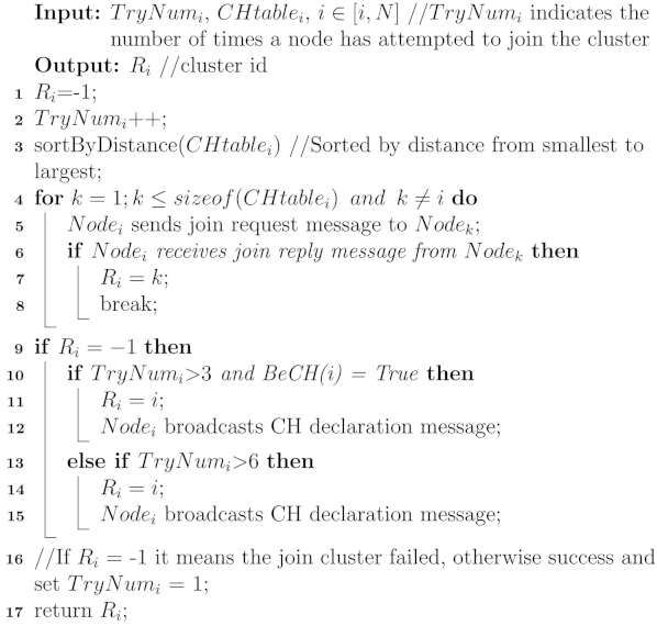
SA state transitions: If there is a CH node around the node, the node sends a JOIN_REQ packet to the CH node to try to join the cluster. If the node receives a JOIN_RESP message from the CH node, the node enters the CM state; the node can determine whether they meet the conditions to become a CH (the conditions to become a CH will be described in detail below) if they have failed multiple attempts to join the cluster, and if so, the node enters the CH state; if the node tries to join the cluster more than six times and does not satisfy the condition to become a CH, the node becomes a CH unconditionally and enters the CH state.

CM state transitions: If the CH information maintained by the node is outdated, it means that the node has left the current cluster, and the node transitions to the SA state; If there is more than one cluster around the node and there is a cluster that is better than the node’s current cluster, then the node will proactively switch to join the better cluster, and the state of the node remains CM at this time; the node will also periodically determine whether the node is better than the current CH node in the cluster, and if so, the node will replace the current CH node and the node state turns to CH.

CH state transitions: If a node receives a REPLACE_REQ packet from a CM node in the cluster, the node abandons the CH state and becomes a CM; if there is no CM node in the cluster managed by the node, the node status turns to SA.

3.4. Utility Calculation Method

In the CH selection process, each node must calculate its utility to determine whether to declare itself as a CH. In this section, we present the method for calculating the utility for a node.

• Group Node Degree Ratio

The group node degree ratio is the ratio of the number of neighboring nodes to the number of group nodes. This factor represents the consistency of the CH node and its neighbor nodes’ direction to ensure the cluster’s stability. It is defined as:

$$D_i(t)=\frac{g_i}{d_i},$$

(3)

where $d_i$ denotes the node degree of node $i$, which is the number of neighboring nodes, and $g_i$ denotes the number of nodes where the angle between node $i$ and its neighbors’ movement direction is less than 90 degrees.

2.

Relative Average Distance of Neighbors

The relative average distance of neighbors is calculated as:

$${\overline{AD}}_i(t)=\frac{{\displaystyle {\sum }_{j\in N(i)}dist(i,j)}}{d_i},$$

(4)

where $dist(i,j)$ is the distance between node $i$ and node $j$.

3.

Relative Average Movement of Neighbors

The relative average movement of neighbors is the movement similarity of a node with its neighbors. This factor represents the future distance between a node and its neighbors. The relative movement of node pairs is calculated as:

$$M_{ij}(t)=\frac{D{N}_{ij}(t)}{D{P}_{ij}(t)},$$

(5)

where $M_{ij}(t)$ is the movement factor between node $i$ and node $j$ at the moment $t$, $D{N}_{ij}(t)$ is the distance between node $i$ and node $j$ at the moment $t$, and $D{P}_{ij}(t)$ represents the relative distance that is predicted with the mobility model between the node pair. The $D{N}_{ij}(t)$ is easily calculated based on the position of node $i$ and node $j$ at time $t$. The node’s movement depends on its surrounding pheromone concentration. It is hard to predict the exact distance between two nodes, so we use mathematical expectation for processing. $D{P}_{ij}(t)$ is calculated as:

$$D{P}_{ij}(t)=\mathrm{sum}\left(M{P}_{ij}(t)\right),$$

(6)

where $sum(.)$ is the function that finds the sum of the elements of the matrix, and $M{P}_{ij}(t)$ can be calculated by:

$$M{P}_{ij}(t)=\left(\begin{array}{c}{V}_{il}(t)\\ V_{is}(t)\\ V_{ir}(t)\end{array}\right)\circ \left(\begin{array}{ccc}{V}_{jl}(t)& V_{js}(t)& V_{jr}(t)\end{array}\right)=\left(\begin{array}{ccc}{V}_{il}(t)\circ V_{jl}(t)& V_{il}(t)\circ V_{js}(t)& V_{il}(t)\circ V_{jr}(t)\\ V_{is}(t)\circ V_{jl}(t)& V_{is}(t)\circ V_{js}(t)& V_{is}(t)\circ V_{jr}(t)\\ V_{ir}(t)\circ V_{jl}(t)& V_{ir}(t)\circ V_{js}(t)& V_{ir}(t)\circ V_{jr}(t)\end{array}\right),$$

(7)

where $V_l(t)$, $V_s(t)$, and $V_r(t)$ denote the information, including predicted position $L(t)$ and probability $P(t)$ calculated based on the pheromone concentration around the node positions in the patrol map of the node after turning left, going straight, and turning right, respectively. $V(t)$ is expressed as $\left(L(t),P(t)\right)$. $M{P}_{ij}(t)$ denotes the distance expectation of node $i$ and node $j$ after turning left, going straight, and turning right, respectively, and finally, a $3\times 3$ distance expectation matrix is obtained. $V_i(t)\circ V_j(t)$ is defined as $\sqrt{{\left(L_i(t)-L_j(t)\right)}^2}\times P_i(t)\times P_j(t)$. Finally, the relative average movement of neighbors is calculated as:

$${\overline{M}}_i(t)=\frac{{\displaystyle \sum _{k=1}^{d_i}{M}_{ij}(t)}}{d_i}.$$

(8)

3.5. Clustering Algorithm

Figure 4 is the BPCA scheme flowchart. This section describes the clustering algorithm proposed in this paper, which consists of four phases: neighbor discovery, CH selection, cluster formation, and cluster maintenance. Most of the processes in the clustering algorithm are repetitive, such as periodically sending hello messages, updating maintenance information, calculating node weights, selecting the optimal cluster, and determining whether the CH node still meets the CH conditions [22]. The periods are shown in

Table 2. Period of repeated tasks in the simulation.

Parameters	Symbols	Values
Hello Period	$T_{hello}$	1.5 s
Update Period	$T_{update}$	$3\times T_{hello}$
Weighting Period	$T_{weighting}$	$5\times T_{hello}$
Alternation Period	$T_{alternation}$	$5\times T_{hello}$
Reselect Period	$T_{reselect}$	$T_{hello}$

, and the usage of each period is described in detail below.

3.5.1. Neighbor Discovery

In the initial network construction phase, each node broadcasts a hello message to the surrounding nodes, which carries some node information, including node location, speed, and node score information. After the neighboring nodes receive the hello message, the nodes parse the message and save the relevant data into the neighbor table.

3.5.2. CH Selection

The CH selection is crucial to ensure the stability of the network topology. Due to the high mobility of UAV networks, the selection of CH is considered from several angles. In this scenario, utility factors, such as group node degree ratio, relative average distance of neighbors, and relative average movement of neighbors, are considered in the CH selection. Since, in this scenario, we assume that the UGV carries sufficient energy for its use as well as to charge the UAV, the energy of the UAV is not considered in the CH selection, limiting the UAV with less than 30% energy to not participating in the CH selection.

Step 1. Each node calculates the value of its utility factors $D_i(t)$, ${\overline{AD}}_i(t)$, and ${\overline{M}}_i(t)$ by its node information and the information maintained in the neighbor table, respectively. The details of the calculation method for each utility factor will be introduced in the following section.

Step 2. Each node calculates the value of its utility, and the utility can be calculated as:

$$\begin{array}{l}{W}_i=D_i(t)\times w_1+\frac{R-{\overline{AD}}_i(t)}{R}\times w_2+\frac{1}{1+e^{-\left({\overline{M}}_i(t)-1\right)}}\times w_3,\\ w_1+w_2+w_3=1,\end{array}$$

(9)

where $R$ denotes the communication range.

Step 3. The neighboring nodes’ utility can be obtained through a hello message. If the node utility is greater than the neighboring nodes’ utility, then the node is the CH node and broadcasts the CH declaration message. Otherwise, it moves to cluster formation.

3.5.3. Cluster Formation

The CH nodes are identified through the CH selection phase, so the normal nodes need to select clusters to join in this phase. Each normal node parses the received CH declaration notification and maintains it in the CH table. The node sends a join request message to the nearest cluster head node, and if the node receives a join reply message from the cluster head node, it successfully joins the cluster. If the node does not join a cluster within $3\times T_{hello}$, the node determines whether it meets the condition to become a CH, and if it does, the node becomes a CH node. If the node does not join a cluster within $6\times T_{hello}$, the node becomes a CH unconditionally. Each node repeats the above steps until each node joins a cluster. At this point, cluster formation is complete. Namely, the network topology is formed. The details of the method are shown in Algorithm 1.

Algorithm 1: Cluster Formation Algorithm

3.5.4. Cluster Maintenance

Due to the high mobility of UAVs, the network topology changes rapidly, such as nodes leaving their clusters and new nodes joining the network. Therefore, the cluster needs to maintain the network topology periodically to ensure the timeliness and connectivity of the network topology. The following describes the cluster maintenance methods in different situations in detail.

• Node Join Cluster

When a new node joins the network or a node in a cluster leaves the cluster, according to the CH table, the node will send a join request message to the nearest CH node, and if the node receives a join reply message from the CH node, it successfully joins the cluster.

2.

Node Leave Cluster

If a node does not receive a hello message from the CH for a long time, it indicates that the node has left the cluster. The node removes the information about the cluster and performs the join cluster operation.

3.

Node maintenance information update

Nodes check the information maintained by themselves for invalid information every $T_{update}$ cycle and delete the invalid information in time to ensure the stability and connectivity of the network topology.

4.

Cluster Head Replacement

Nodes per $T_{alternation}$ determine whether the node’s utility is greater than the utility of the current CH by $\in$, where $\in$ is a design parameter and defined as 10% of the current cluster head’s utility. If it is greater than that, the node becomes the cluster head. Other cluster members are still members of the cluster if they are neighbors of the new cluster head. Otherwise, they become normal nodes for the join cluster operation.

5.

Cluster Replacement

The node chooses the nearest cluster to join every $T_{reselect}$ cycle, sends a join request message to the nearest cluster head node around, and if the node receives a join reply message from the cluster head node, it joins the cluster successfully.

4. Simulation and Discussion

In this section, we set up a simulated simulation environment to evaluate the performance and effectiveness of our proposed algorithm.

4.1. Simulation Setup

This paper simulates the scheme (BPCA) in the discrete simulator NS3.0 network simulation software. The size of the simulation area is $1000\mathrm{m}\times 1000\mathrm{m}$, and the nodes are randomly distributed in the area. We use the IEEE 802.11b radio standards for wireless communication. IEEE 802.11b, which operates in the 2.4-GHz frequency band, supports 200–250 m of outdoor coverage and a maximum transmission speed of 11 Mb/s. The parameters of each node are initialized identically, where the communication radius range of the nodes is $200\mathrm{m}$. The patrol mobility model is used to simulate the node movement behavior, and the maximum speed of the nodes is taken to be in the range of $10–40\mathrm{m}/\mathrm{s}$, where the minimum speed is $0\mathrm{m}/\mathrm{s}$. The speed difference between nodes will increase as the maximum speed increases. The change in speed difference simulates the drastic network topology change to verify the performance of our algorithm. We set the weight as $w_1=0.08$, $w_2=0.07$, and $w_3=0.85$, and each simulation time is $60\mathrm{s}$. The detailed simulation parameters are shown in

Table 3. The values of the simulation parameters.

Parameters	Values
Simulation time (s)	$60$
Size of topology (m)	$1000\times 1000$
Max speed (m/s)	$10, 20, 30, 40$
Number of AV	$100, 150, 200$
Number of GV	$1$
Transmission range (m)	$200$
Mac channel	MAC/802.11b
Propagating model	Long distance propagation loss model
Error model	YANS
Mobility model	patrol mobility model [6]
Number of trials	$300$

.

To illustrate the efficiency of our scheme, the algorithm in this paper will be compared with three state-of-the-art weighted clustering algorithms for ad-hoc networks, namely, adaptive enhanced weighted clustering algorithm (AEWCA) [23], weighted clustering algorithm (WCA) [8], and dependability-based clustering algorithm (DCA) [22]. WCA is the classical weighted clustering algorithm. In the clustering process, the WCA scheme considers various factors of nodes, such as energy and speed, but does not consider the relative speed of movement direction between nodes. The AEWCA is a weighted clustering algorithm that improves the WCA scheme. The algorithm considers utility factors, such as node degree, internode distance, average link retention time, and energy consumption in the clustering process. The DCA scheme is a dependency-based clustered routing algorithm. The DCA scheme focuses on the dependability of clusters rather than considering only individual nodes to maintain the clustered structure of a network. The node joins the cluster with the highest dependency score of the surrounding clusters, thus, improving the stability of the cluster, but the dependency score computation is costly.

In the simulation, we take the weight of AEWCA as $w_1=0.45$, $w_2=0.45$, and $w_3=0.1$, the weight of WCA as $w_1=0.2$, $w_2=0.2$, $w_3=0.5$, and $w_4=0.1$, and the weight of DCA as $w_1=0.45$, $w_2=0.45$, and $w_3=0.1$, respectively, so that the best results can be obtained. A large number of simulations were conducted by varying the maximum speed of movement of the nodes and the number of nodes while keeping other conditions constant. Three hundred simulations were performed for each case, and the simulation results were averaged.

4.2. Simulation Results

The average CH duration time, average CM duration time, the average number of CM changes, the average number of CM changes, and the average number of standalone nodes can effectively evaluate the stability of the cluster and the reliability of link. By comparing the five indicators, we get the following simulation results.

(1)

The average CH duration time

The average CH duration time indicates the average time that the node is in the CH state during the simulation. The average CH duration time can be obtained by the following formula:

$$AvgR{T}_{CH}=\frac{{\displaystyle \sum _{i=0}^{n}R{T}_{CH}(i)}}{n},$$

(10)

where $AvgR{T}_{CH}$ denotes the average CH duration time, n denotes the number of nodes that come into the CH state, and $R{T}_{CH}(i)$ denotes the cluster head retention time of node $i$. After the simulation, the simulation results were captured and are shown in Figure 5.

Figure 5 represents the relationship between the average CH duration time and a node’s maximum movement speed, where Figure 5a–c represent the case when the number of nodes is 100, 150, and 200, respectively. It can be first seen in Figure 5 that the average CH duration time of the nodes tends to decrease as the node speed increases. Then, when the number of nodes is 100, the average CH duration time of the BPCA scheme proposed in this paper is lower than that of AEWCA. As the number of nodes increases, the average CH duration time of the BPCA scheme gradually improves and outperforms other algorithms.

(2)

The average CM duration time

The average CM duration time indicates the average time that a node is in the CM state during the simulation. The calculation of this metric is similar to the calculation of the average CH duration time. The simulation results are shown in Figure 6.

Figure 6 represents the relationship between the average CM duration time and a node’s maximum movement speed. Firstly, it can be seen in Figure 6 that the average CM duration time decreases with increasing speed, where the BPCA scheme performs best, followed by DCA. In addition, the average CM duration time of the BPCA scheme increases as the number of nodes in the network increases.

(3)

The average number of CM detached from clusters

The average number of CM detached from clusters is the number of times a node breaks away from its cluster due to the dramatic movement of the CM node. The simulation results are shown in Figure 7.

Figure 7 represents the relationship between the average number of CM detached from clusters and a node’s maximum movement speed. It can be seen in Figure 7 that the number of the average number of CM detached from clusters increases with the increasing number of nodes and node speed. The average number of CMs that breaks away from clusters in the BPCA scheme is the lowest compared to other algorithms.

(4)

The average number of CM changes

The number of CM changes includes the number of times a CM node actively joins other clusters and the number of times a CM node leaves its cluster. The simulation results are shown in Figure 8.

Figure 8 represents the relationship between the average number of CM changes and a node’s maximum movement speed. As can be seen in Figure 8, the average number of CM changes increases as the speed and the number of nodes increase. The average number of CM changes in the BPCA scheme and DCA scheme is much higher than the average number of CM changes in the WCA and AEWCA schemes, where the number of changes in BPCA is smaller than that of DCA.

(5)

The average number of standalone nodes

The average number of standalone nodes can be obtained by the following formula:

$$Av{g}_{SA}=\frac{{\displaystyle \sum _{i=0}^{k}SA(i)}}{k},$$

(11)

where $Av{g}_{SA}$ denotes the average number of standalone nodes, $k$ denotes the number of samples taken in the simulation, and $SA(i)$ denotes the number of standalone nodes at the i-th sampling. The simulation results are shown in Figure 9.

Figure 9 represents the relationship between the average number of standalone nodes and a node’s maximum movement speed. It can be seen in Figure 9 that the average number of standalone nodes increases with increasing speed, where the BPCA scheme performs the best.

4.3. Results Discussion

As the speed of nodes increases, the network topology changes drastically, which leads to an increase in the state changes of nodes. The number of changes in CH and CM increases, resulting in a decrease in the average duration time of CH and CM. The frequent disconnection of links leads to an increase in standalone nodes. From the simulation results, the above analysis can be verified.

As shown in Figure 5a, the average CH duration time of BPCA is lower than AEWCA. Since BPCA and DCA use the same cluster maintenance strategy, where CM nodes periodically determine whether they can replace the CH node in the current cluster, therefore, compared to WCA and AEWCA schemes, the number of node changes in CH will be increased, resulting in a decrease in the average cluster head retention time. As shown in Figure 5b,c, as the number of nodes increases, the average CH duration time of the BPCA scheme gradually improves and outperforms other algorithms. Due to the fact that as the number of nodes increases, the node weights become less affected by a node’s movement changes, thus, the number of state changes in CH decreases, and the average CH duration time of nodes increases.

As shown in Figure 8, the cluster maintenance strategy of the BPCA scheme and DCA scheme CM nodes will actively try to join the surrounding optimal clusters, so the average number of CM changes in the BPCA scheme and DCA scheme is much higher than the average number of CM changes in the WCA and AEWCA schemes, but most of them are the number of CM intercluster switches. As can be seen in Figure 7, the number of CM nodes passively detaching from clusters in BPCA is lower than other algorithms due to the superior maintenance policy, which greatly improves the stability of the network topology.

The BPCA scheme considers the direction between nodes and the distance between the current and the next moment in CH selection, so the selected CHs are more closely related to the nodes in the cluster. We estimate the distance between nodes at the next moment based on the probability of each node’s following movement behavior, and this calculation method is more applicable. It can be seen from the simulation results that the BPCA scheme outperforms other algorithms, thus, confirming the effectiveness of our algorithm.

5. Mobility Model Discussion

In ad-hoc network simulation, a realistic simulation environment is created by using appropriate mobility models according to different scenarios. Studies have shown that the performance of routing protocols varies significantly over various mobility model scenarios [26]. Therefore, understanding the characteristics and selecting the appropriate mobility model is crucial for obtaining valuable conclusions from the simulation results. In the following, several mobility models that have been proposed are presented.

Random Waypoint (RWP) Mobility Model [27]: this mobility model periodically selects a random target location and moves toward the target at a randomly selected speed, and then, repeats the process.

Random Direction (RD) Mobility Model [28]: Unlike the RWP scheme, this mobility model’s strategy is to move in a randomly chosen direction until the node reaches the edge of the simulated area and then repeat the above process. The RWP and RD mobility models are simple to implement, but the sudden change in direction is not a typical movement characteristic of UAVs, and simulating FANET has limitations.

Gauss–Markov (GM) Mobility Model [29]: In the GM mobility model, nodes will be assigned a random velocity and direction in the initial phase, and subsequently, the velocity and direction of the nodes will be updated at intervals based on the previous velocity and direction of the nodes. Since the movement trajectory of the GM mobility model is randomly unpredictable, the model can be used in patrol scenarios. However, the mobility model does not consider spatial correlation, which leads to low-patrol efficiency.

Smooth-Turn (ST) Mobility Model [30]: In the ST mobility scheme, the node is rotated with a randomly selected turn point perpendicular to the current direction of movement as the center of the circle, and the next turn point is selected after maintaining a duration that matches the exponential distribution. The turning of this mobility model is very smooth and conforms to the UAV movement characteristics. The mobility model is suitable for patrol scenarios, but the implementation is more complicated.

Our proposed clustering scheme is unsuitable for the RWP and RD mobility models because both models do not conform to the movement characteristics of UAVs and the node movement direction changes drastically. Thus, the calculated utility factor ${\overline{M}}_i(t)$ deviates significantly from the actual value. The GM and ST mobility models can calculate ${\overline{M}}_i(t)$ by using the movement strategy of the mobility model that can directly predict the node’s position at the next moment. The GM and ST mobility models conform to the UAV movement characteristics, and the nodes can also calculate the probability of nodes turning left, moving straight, and turning right by the movement strategy of the mobility model, and thus calculate the ${\overline{M}}_i(t)$. Our proposed clustering strategy is suitable for a mobility model that conforms to the movement characteristics of UAVs.

6. Conclusions

In this paper, we proposed a clustering algorithm based on the ground-air cooperative architecture in border patrol scenarios. The ground-air cooperative network consists of UGVs and UAVs, where the UGVs provide services to the UAVs, greatly increasing the network’s survival time and the patrol range of the UAVs. The clustering algorithm is improved in terms of selecting cluster utility factors and calculating factors. In selecting CH, we considered three utility factors in selecting CH: the group node degree ratio, the relative average distance of neighbors, and the relative average movement of neighbors. The simulations show that the algorithm improves the stability of the cluster and the reliability of the link. In future research, the applicability of our proposed algorithm in different scenarios should be studied in detail.

References

- Lin, N.; Fu, L.; Zhao, L.; Min, G.; Al-Dubai, A.; Gacanin, H. A Novel Multimodal Collaborative Drone-Assisted VANET Networking Model. IEEE Trans. Wirel. Commun. 2020, 19, 4919–4933. [Google Scholar] [CrossRef]
- Cal, Y.F.; Sekiyama, K.; IEEE. Geometric Relation Matching based Object Identification for UAV and UGV Cooperation. In Proceedings of the Conference on Technologies and Applications of Artificial Intelligence (TAAI), Tainan, Taiwan, 20–22 November 2015; IEEE: Tainan, Taiwan, 2015. [Google Scholar]
- Stentz, T.; Kelly, A.; Herman, H.; Rander, P.; Amidi, O.; Mandelbaum, R. Integrated Air/Ground Vehicle System for Semi-Autonomous Off-Road Navigation; The Robotics Institute: Pittsburgh, PA, USA, 2002. [Google Scholar]
- Liu, Y.; Liu, Z.; Shi, J.; Wu, G.; Chen, C. Optimization of Base Location and Patrol Routes for Unmanned Aerial Vehicles in Border Intelligence, Surveillance, and Reconnaissance. J. Adv. Transp. 2019, 2019, 13. [Google Scholar] [CrossRef]
- Bekmezci, I.; Sahingoz, O.K.; Temel, S. Flying Ad-Hoc Networks (FANETs): A survey. Ad. Hoc. Netw. 2013, 11, 1254–1270. [Google Scholar] [CrossRef]
- Kuiper, E.; Nadjm-Tehrani, S. Mobility models for UAV group reconnaissance applications. In Proceedings of the 2006 2nd International Conference on Wireless and Mobile Communications, Bucharest, Romania, 29–31 July 2007; pp. 180–186. [Google Scholar]
- Gerla, M.; Tsai, J.T.C. Multicluster, mobile, multimedia radio network. Wirel. Netw. 1995, 1, 255–265. [Google Scholar] [CrossRef]
- Chatterjee, M.; Das, S.K.; Turgut, D. WCA: A weighted clustering algorithm for mobile ad hoc networks. Clust. Comput. 2002, 5, 193–204. [Google Scholar] [CrossRef]
- Chinara, S.; Rath, S.K. Mobility Based Clustering Algorithm and the Energy Consumption Model of Dynamic Nodes in Mobile Ad Hoc Network. In Proceedings of the 11th International Conference on Information Technology, Bhubaneswar, India, 17–20 December 2008; IEEE Computer Soc: Bhubaneswar, India, 2008. [Google Scholar]
- Ucar, S.; Ergen, S.C.; Ozkasap, O. VMaSC: Vehicular Multi-hop algorithm for Stable Clustering in Vehicular Ad Hoc Networks. In Proceedings of the IEEE Wireless Communications and Networking Conference (WCNC), Shanghai, China, 7–10 April 2013; IEEE: Shanghai, China, 2013. [Google Scholar]
- Sun, G.; Qin, D.; Lan, T.; Ma, L. Research on Clustering Routing Protocol Based on Improved PSO in FANET. IEEE Sens. J. 2021, 21, 27168–27185. [Google Scholar] [CrossRef]
- Arafat, M.Y.; Moh, S. Localization and Clustering Based on Swarm Intelligence in UAV Networks for Emergency Communications. IEEE Internet Things J. 2019, 6, 8958–8976. [Google Scholar] [CrossRef]
- Sefati, S.S.; Halunga, S.; Farkhady, R.Z. Cluster selection for load balancing in flying ad hoc networks using an optimal low-energy adaptive clustering hierarchy based on optimization approach. Aircr. Eng. Aerosp. Technol. 2022; ahead-of-print. [Google Scholar] [CrossRef]
- Medani, K.; Guemer, H.; Aliouat, Z.; Harous, S. Area Division Cluster-based Algorithm for Data Collection over UAV Networks. In Proceedings of the IEEE International Conference on Electro Information Technology (EIT), Mount Pleasant, MI, USA, 14–15 May 2021; IEEE: Mount Pleasant, MI, USA, 2021. [Google Scholar]
- Wang, J.; Zhang, Q.; Feng, G.; Qin, S.; Zhou, J.; Cheng, L. Clustering Strategy of UAV Network Based on Deep Q-learning. In Proceedings of the 2020 IEEE 20th International Conference on Communication Technology (ICCT), Nanning, China, 28–31 October 2020; pp. 1684–1689. [Google Scholar]
- Yang, X.; Yu, T.; Chen, Z.; Yang, J.; Hu, J.; Wu, Y. An Improved Weighted and Location-Based Clustering Scheme for Flying Ad Hoc Networks. Sensors 2022, 22, 3236. [Google Scholar] [CrossRef]
- Haider, S.K.; Jiang, A.; Almogren, A.; Rehman, A.U.; Ahmed, A.; Khan, W.U.; Hamam, H. Energy Efficient UAV Flight Path Model for Cluster Head Selection in Next-Generation Wireless Sensor Networks. Sensors 2021, 21, 8445. [Google Scholar] [CrossRef] [PubMed]
- Ma, T.; Zhou, H.; Qian, B.; Fu, A. A large-scale clustering and 3D trajectory optimization approach for UAV swarms. Sci. China-Inf. Sci. 2021, 64, 16. [Google Scholar] [CrossRef]
- Cai, M.; Rui, L.; Liu, D.; Huang, H.; Qiu, X. Group Mobility Based Clustering Algorithm for Mobile Ad Hoc Networks. In Proceedings of the 17th Asia-Pacific Network Operations and Management Symposium APNOMS 2015, Busan, Korea, 19–21 August 2015; IEEE: Busan, South Korea, 2015. [Google Scholar]
- Du, J.; You, Q.; Zhang, Q.; Xin, X.; Tian, Q.; Cao, G.; Liu, B.; Zhang, L.; Tao, Y.; Tian, F.; et al. A weighted clustering algorithm based on node stability for Ad Hoc Networks. In Proceedings of the 2017 16th International Conference on Optical Communications and Networks (ICOCN), Wuzhen, China, 7–10 August 2017; p. 3. [Google Scholar]
- Guo, J.; Gao, H.; Liu, Z.; Huang, F.; Zhang, J.; Li, X.; Ma, J. ICRA: An Intelligent Clustering Routing Approach for UAV Ad Hoc Networks. IEEE Trans. Intell. Transp. Syst. 2022, 1–14. [Google Scholar] [CrossRef]
- Ergenc, D.; Eksert, L.; Onur, E. Dependability-based clustering in mobile ad-hoc networks. Ad Hoc Netw. 2019, 93, 25. [Google Scholar] [CrossRef]
- Sun, Y.; Mi, Z.; Wang, H.; Lu, F.; Zhao, N. Adaptive Enhanced Weighted Clustering Algorithm for UAV Swarm. In Proceedings of the 2020 IEEE 20th International Conference on Communication Technology (ICCT), Nanning, China, 28–31 October 2020; pp. 709–714. [Google Scholar]
- Ye, L.; Zhang, Y.; Li, Y.; Han, S. A Dynamic Cluster Head Selecting Algorithm for UAV Ad Hoc Networks. In Proceedings of the 2020 International Wireless Communications and Mobile Computing (IWCMC), Limassol, Cyprus, 15–19 June 2020; pp. 225–228. [Google Scholar]
- Wang, X.; Liu, Z.; Jian, C.; Shi, S.; Gu, J.; Shi, F. A Dynamic Scale UAV Weighted Clustering Algorithm. In Proceedings of the 2021 IEEE International Conference on Unmanned Systems (ICUS), Beijing, China, 15–17 October 2021; pp. 209–213. [Google Scholar]
- Ravikiran, G.; Singh, S. Influence of mobility models on the performance of routing protocols in ad-hoc wireless networks. In Proceedings of the 2004 IEEE 59th Vehicular Technology Conference, VTC 2004-Spring (IEEE Cat. No.04CH37514), Milan, Italy, 17–19 May 2004; Volume 4, pp. 2185–2189. [Google Scholar]
- Johnson, D.B.; Maltz, D.A. Dynamic Source Routing in Ad Hoc Wireless Networks. In Mobile Computing; Imielinski, T., Korth, H., Eds.; Kluwer Academic Publishers: Dordrecht, The Netherlands, 1996; pp. 153–181. [Google Scholar]
- Royer, E.M.; Melliar-Smith, P.M.; Moser, L.E. An analysis of the optimum node density for ad hoc mobile networks. In Proceedings of the ICC 2001, IEEE International Conference on Communications, Conference Record (Cat. No.01CH37240), Helsinki, Finland, 11–14 June 2001; Volume 3, pp. 857–861. [Google Scholar]
- Liang, B.; Haas, Z. Predictive Distance-based Mobility Management for PCS Networks. In Proceedings of the IEEE INFOCOM 1999, New York, NY, USA, 21–25 March 1999; Volume 3, pp. 1377–1384. [Google Scholar]
- Wan, Y.; Namuduri, K.; Zhou, Y.; Fu, S. A Smooth-Turn Mobility Model for Airborne Networks. In IEEE Transactions on Vehicular Technology; IEEE: Washington, DC, USA, 2013; Volume 62, pp. 3359–3370. [Google Scholar]
Publisher’s Note: MDPI stays neutral with regard to jurisdictional claims in published maps and institutional affiliations. |
© 2022 by the authors. Licensee MDPI, Basel, Switzerland. This article is an open access article distributed under the terms and conditions of the Creative Commons Attribution (CC BY) license (https://creativecommons.org/licenses/by/4.0/).