A Piece-Wise Linear Model-Based Algorithm for the Identification of Nonlinear Models in Real-World Applications

Abstract

In this work, a data-driven approach for the identification of a piece-wise linear model for nitrogen oxide daily concentration simulation is presented and applied. The model has been identified by using daily measured concentrations, meteorological variables, and emission levels estimated starting from the results contained in suitable emission databases. We propose an innovative methodology that jointly optimizes clustering and parameter identification. The procedure has been applied considering data from the Milan (Italy) metropolitan area. The methodology has been compared with two state-of-the-art approaches based on a two-step, cluster-based algorithm and on Hammerstein–Wiener models. The results show how, in the presented application, the devised approach ensures better performance with respect to the two literature methods, both in terms of statistical indexes (correlation, normalized mean absolute error) and in terms of problem-specific metrics (hit ratio, false alarm). For this reason, the approach can be considered suitable to be used in the definition of optimal emission control strategies.

1. Introduction

Due to negative impacts on human health [1,2], the exposure to high daily concentrations of nitrogen dioxide (NO${}_2$) has become one of the most important environmental problems for regional and local authorities as well as companies (see, for instance, the introduction of optimization strategies to reduce pollution in last-mile delivery [3,4]). In this context, the European Legislation has defined challenging atmospheric concentration thresholds that should not be exceeded, both as daily maximum value (200 μg/m${}^3$ that can be violated for at most 18 times in a year) and annual mean (40 μg/m${}^3$). Control theory can grant authorities both theoretical and practical tools to find a set of suitable short and long-term strategies complying with these constraints due to the fact that the NO${}_2$ dynamic in the atmosphere is driven by complex and nonlinear phenomena involving chemical reactions, anthropogenic and biogenic emission, and meteorological conditions (in particular solar radiation and wind speed and direction) [5]. The inter-relationship among different areas of interest (i.e., chemistry, meteorology) has led the literature to focus on increasingly complex deterministic systems of systems aimed at the description of the atmospheric phenomena over a predefined geographical domain [6,7,8,9,10,11]. Unfortunately, the complexity of these systems implies computational times that are not compatible with the phase of control system development, often performed solving optimization problems through numerical algorithms. For these reasons, it is necessary to identify simplified models describing the relationships among daily concentrations, emissions, and meteorological conditions. Therefore, the pure use of models obtained through the analytical simplification of the full model or through a surrogate modeling approach does not ensure performance compatible to the aforementioned aims [12,13]. In this work, the problem is approached by identifying a data-driven model that links the concentrations measured by the environmental stations, meteorological conditions, and estimated emissions. In the literature, a number of approaches have been proposed to represent nonlinear complex systems on the basis of data and/or limited information [13,14,15,16], sometimes presenting applications on the analysis and control of variables in the real world [17,18,19]. One of the main points arising from these works and strictly connected to the representation of complex systems as the natural ones, is related to what can be presented as the curse of model complexity. In order to represent the complex system a complex model is usually needed, but this can lead to a very challenging and sometimes not solvable control design problem. For this reason, in order to take into account the non-linearity of the involved phenomena and to limit the complexity of the models, a piece-wise linear model (PLM) approach is often used [20]. In the literature, a number of works about PLM identification are presented [20,21,22,23]. Usually, PLM starts from the identification and use of a linear model for each region into which the input space can be divided, defined as the cartesian products of the intervals in which the different model input can be split. This entails a large number of models when the number of inputs is high, making (1) the solution of the identification problem very challenging and time-consuming, and (2) the resulting overall model very complex. Recently, a combined approach of clustering and PLM has been used in [24,25] for the implementation of a forecasting system.

In this work, a sequential quadratic programming algorithm, as presented in [26], is used to identify a piece-wise linear model jointly optimizing clustering (centroid coordinates) and parameter values. In this condition, the clustering phase, performed by k-means [27], is applied only to provide the initial condition of the numerical algorithm.

Table 1. Comparison of this paper with related literature papers.

Paper	Approach	Model Type	Minimized	MIMO	Real World
			Error	Applicability	Applications
Dolanc and Strmcnik, 2005 [20]	Fixed Intervals + RLS with forgetting factor	Hammerstein	Forecasting	-	-
Ipanaque and Manrique, 2011 [22]	2 step: interval definition + Recursive Least Square	Wiener	Forecasting	-	PH control
Westra et al., 2011 [23]	Fixed intervals + model parameter estimation based on optimization algorithm	State Space + discrete state	Forecasting	MIMO	-
Zhang et al., 2018 [28]	Online clustering + Least Square	Hammerstein	Forecasting	MIMO	Stirred track control
Lassoued and Abderrahim, 2019 [29]	Static Clustering based on SVM reconstruction of regions + least square	PWARX	Forecasting	MISO	-
Yang et al., 2019 [24]	Plane clustering (number of plane selected through optimization algorithm)	Non dynamical regression	Regression error	-	UCI data
Hadid et al., 2020 [21]	Static Clustering + Least Square	PWARX	Forecasting	MISO	River flood
Liu et al., 2022 [25]	Time partitioning + optimal identification	PWARX	Forecasting	MISO	Injection Molding
Carnevale et al., this work	Full dynamical selection of cluster centroids + constrained optimization	PWARX	Simulation	MISO	Air quality simulation

presents a comparison between the presented work and the most related works available in the literature, as far as is known by the authors. The main contributions provided by this work are: (i) the use of a joint approach provides a more flexible methodology not entirely dependent on the clustering procedure. The method allows us to tackle the piece-wise linear model identification problem using as unique clustering information the number of regions of the input space (since the centroids are variables of the model) (ii) the identification based on the optimization of the simulation error while complying with constraints caused by the relationship between input and output variables; (iii) the application of the model to a strong complex and nonlinear real-world system. Moreover, due to the limited assumption on input and output data, the methodology is general enough to be applied to Multi-InputMulti-Output (MIMO) systems, even if the presented application is focused on a Multi-Input-Single-Output (MISO) system. The work can be considered as the first step needed to develop and implement a suitable pollution control problem. The methodology is applied and tested to the simulation of nitrogen oxide (NO${}_2$) concentration in the Milan metropolitan area (Lombardy region, Italy), one of the most polluted areas in Europe.

The paper is organized as follows. In the next section, we introduce the new methodology and we discuss the main implementation details. In Section 3, we compare our method with other relevant approaches in the literature.

2. Methodology

The presented methodology is based on the identification of a piece-wise linear model in the form:

$$y_t=\left\{\begin{array}{cc}\hfill {\theta }^1{x}_t,& \hfill x_t\in G_1\\ \hfill \dots & \hfill \dots \\ \hfill {\theta }^K{x}_t,& \hfill x_t\in G_K\end{array}\right.$$

(1)

where:

• $y_t$ is the output of the model at time t;
• $x_t$ is the input vector of the model at time t, including both the autoregressive and the exogenous parts;
• $G_1$, …, $G_K$ are the regions into which the input space $x_t$ is divided and are used to select the parameters to compute the output of the model at time t;
• ${\theta }^1$, …, ${\theta }^K$ are the parameter vectors to be estimated during the identification phase, with each vector ${\theta }^i$ associated with region $G_i$.

In the real-world phenomena representation through linear systems it can often happen that, due to non-linearity and time dependency, the estimated parameters change on the basis of the value of the input $x_t$. From the theoretical and practical point of view, the identification of this kind of model is very complex if all the possible configurations (different model structure, definition of each region $G_i$ contextually to the parameter vector ${\theta }^i$, $i=1,\cdots ,K$) are considered simultaneously along with the minimization of the simulation error (output $y_t$ at time t is dependent on the model outputs computed at time $\tilde{t}<t$, thus leading to a nonlinear optimization problem) and the satisfaction of constraints [20,23]. For this reason, the existing procedures are frequently based on a crude and simple idea consisting of two steps: in the first one, the regions $G_i,i=1,\cdots ,K$ are defined, sometimes applying clustering techniques to the input data or taking advantage of the knowledge of the involved phenomena, whereas, in the second phase, the estimation of the parameters ${\theta }^1$, …, ${\theta }^K$ is performed. This approach generally requires some restricting conditions such as (i) the number of the regions K is fixed, (ii) the regions are defined before the parameters estimation, and (iii) all the models have the same structure (the autoregressive order of the output and of each exogenous input is fixed). In this work, the methodology aims to address some of these restrictions. Instead of introducing a separated phase for the clustering, the approach exploits a mathematical model where, in addition to variables associated with the parameters to be identified, new variables representing region centroids are defined. In this case, the only clustering information required by the model is the number of regions.

This way, the mathematical model jointly performs the parameters estimation and the clustering, guaranteeing more flexibility and (potentially) better performance with respect to the aforementioned two-step approaches with fixed clustering. Issues (i) and (iii) are treated by performing different tests varying K and the structure of $x_t$. Then, the identification phase is performed through the following optimization problem:

$$\begin{array}{cc}\hfill & \underset{[{\theta }^i,c^i]}{min}\sum _{t=1}^N{(y_t-{\overline{y}}_t)}^2\hfill \\ \hfill & \mathrm{s}.\mathrm{t}.\hfill \end{array}$$

(2)

$$\begin{array}{cc}\hfill & y_t=\sum _{i=1}^{K}g(x_t,c^i)·{\theta }^i·x_t,t=1,\dots ,N;\hfill \end{array}$$

(3)

$$\begin{array}{cc}\hfill & x_t=[y_{t-1},\dots ,y_{t-n_a};{\overline{u}}_t^l,\dots ,{\overline{u}}_{t-n_l}^l,l=1,\cdots ,L]t=1,\cdots ,N;\hfill \end{array}$$

(4)

$$\begin{array}{cc}\hfill & L{B}_{{\theta }^i}<{\theta }^i<U{B}_{{\theta }^i}\hfill \end{array}$$

(5)

$$\begin{array}{cc}\hfill & L{B}_{c^i}<c^i<U{B}_{c^i}\hfill \end{array}$$

(6)

where:

-

K is the number of regions;

-

N is the number of considered time instants (tuples in the identification dataset);

-

${\overline{y}}_t$ is the measured data of the output model at time t;

-

${\overline{u}}_t^l$ is the value of the exogenous input l at time t;

-

$n_a$ is the autoregressive order of the linear systems;

-

$n_l$ is the exogenous order of the l-th input of the linear systems;

-

L is the number of the exogenous inputs of the different models;

-

$L{B}_{{\theta }^i}$, $U{B}_{{\theta }^i}$, $L{B}_{c^i}$, $U{B}_{c^i}$ are the lower and upper bound for the decision variables;

-

$y_t$ is the output at time t;

-

$x_t$ is the input vector of the model, including both the previous output values ($y_{t-1},\dots ,y_{t-n_a}$) and the measured input values (${\overline{u}}_t^l,\dots ,{\overline{u}}_{t-n_l}^l,l=1,\cdots ,L$);

-

${\theta }^i$ are the parameters of the i-th model to be estimated;

-

$c^i$ are the centroids of the different clusters (to be optimized during the identification);

-

$g(x_t,c_i)$ is a check function that determines if $x_t$ belongs to region i, based on a distance measure.

In the presented problem, the objective function (2) minimizes the Euclidean distance between the output of the overall model and the measured data. Equations (3) and (4) represent the model dynamic. It has to be stressed that each model identified per region is linear (Equation (3)) and that, thanks to check function $g(x_t,c^i)$, only one model ${\theta }^i{x}_t$ (the model associated with the centroid $c^i$ closest to the input $x_t$) is “active” for the computation of the output at time t. More precisely, check function $g(x_t,c^i)$ can be defined as follows:

$$g(x_t,c^i)=\left\{\begin{array}{cc}\hfill 1,& \hfill D(x_t,c^i)<D(x_t,c^j)\forall j\ne i\\ \hfill 0,& \hfill otherwise\end{array}\right.$$

where $D(x_t,c^i)$ represents the distance of $x_t$ from the centroid $c^i$. The region associated with the minimum distance value identifies which model has to be activated.

When dealing with the mathematical model (2)–(6) some issues arise: (a) the problem aims to minimize the simulation error (see the presence of the previous output values, and not the previous output measurement, in $x_t$), thus the problem is intrinsically nonlinear. Since the classic least-square approach cannot be used, the problem can be solved through the use of numerical algorithms [26] that usually need an initial condition, i.e., the starting value of the decision variable vector $[{\theta }^i,c^i]$. The latter is particularly critical for centroids optimization. A possible way to find a good initial condition could be through the use of a clustering algorithm. In this case, the clustering phase assumes a different role with respect to what happens in a classical two-step approach, where the resulting cluster procedure statically defines the regions $G_i$ of the piece-wise linear model [21]. (b) The distance $D(x_t,c^i)$ of $x_t$ from the centroid $c^i$ can be computed using the Euclidean distance or any other, more complex, distance such as the Mahalanobis or the Pearson one.

More in detail, in this work, a Euclidean distance is used for the definition of $D(x_t,c^i)$ and the resulting optimization problem is solved by means of the sequential quadratic programming algorithm for nonlinear constrained problems [26] implemented as in [30]. The Algorithm 1 is used to compute the objective function each time new values for the decision variables ${\theta }^i$ (models parameters) and $c_i$ (centroid positions) are defined by the adopted numerical algorithm. Finally, the clustering algorithm used to compute the algorithm’s initial condition for the centroids is the k-means approach [27]. We name clusterOpt the full joint methodology that includes the mathematical model and the algorithm used for its solution. In the next section, the described approach is applied to the Milan metropolitan area, in order to model the daily average concentration of NO${}_2$. We decided to compare clusterOpt with two different state-of-the-art procedures based on (i) a two-step procedure (named cluster) where regions definition is provided by the clustering technique at hand, and a simplified linear model is solved for each of them and (ii) a set of Hammerstein–Wiener models [20].

Algorithm 1 Objective function

$y_1\leftarrow {\overline{y}}_1$ $y_2\leftarrow {\overline{y}}_2$ … $y_{n_a}\leftarrow {\overline{y}}_{n_a}$ for $t=n_a+1:N$ do     $x_t\leftarrow [y_{t-1},\dots ,y_{t-n_a};{\overline{u}}_k^l,\dots ,{\overline{u}}_{k-n_l}^l,l=1,\dots ,L]$     $y_t\leftarrow 0$     for $i=1:K$ do         $\overline{g}\leftarrow g(x_t,c^i)$         $y_t\leftarrow y_t+\overline{g}·{\theta }^i·x_t$     end for end for

3. Experimental Results

The methodology clusterOpt has been applied to model the daily average concentration of nitrogen oxides (NO${}_2$) in the Milan metropolitan area. The daily mean concentration (the model output) is computed as the average of the daily values measured by 12 monitoring stations placed in the area under study. The input dataset includes nitrogen oxides (NO${}_x$) daily total emissions (estimated starting from the INEMAR regional emission inventory [31]) and the measured daily mean temperature, humidity, and solar radiation. The data have been collected for the years 2014–2020. The data-driven model parameters are estimated using the data from 2014 to 2018 (i.e., N is equal to 1826), while the years 2019–2020 have been used for the validation. Five different solution methods have been compared:

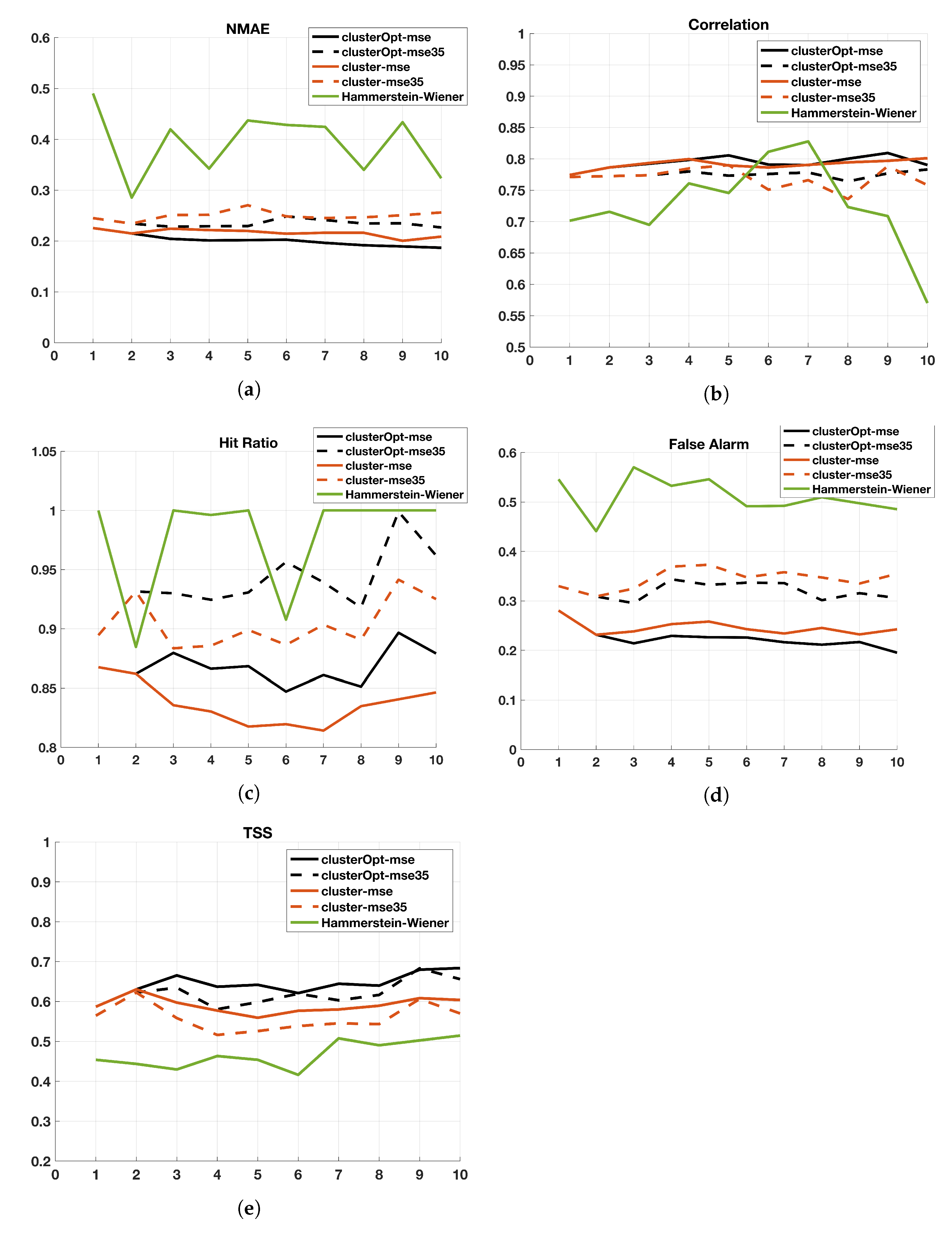
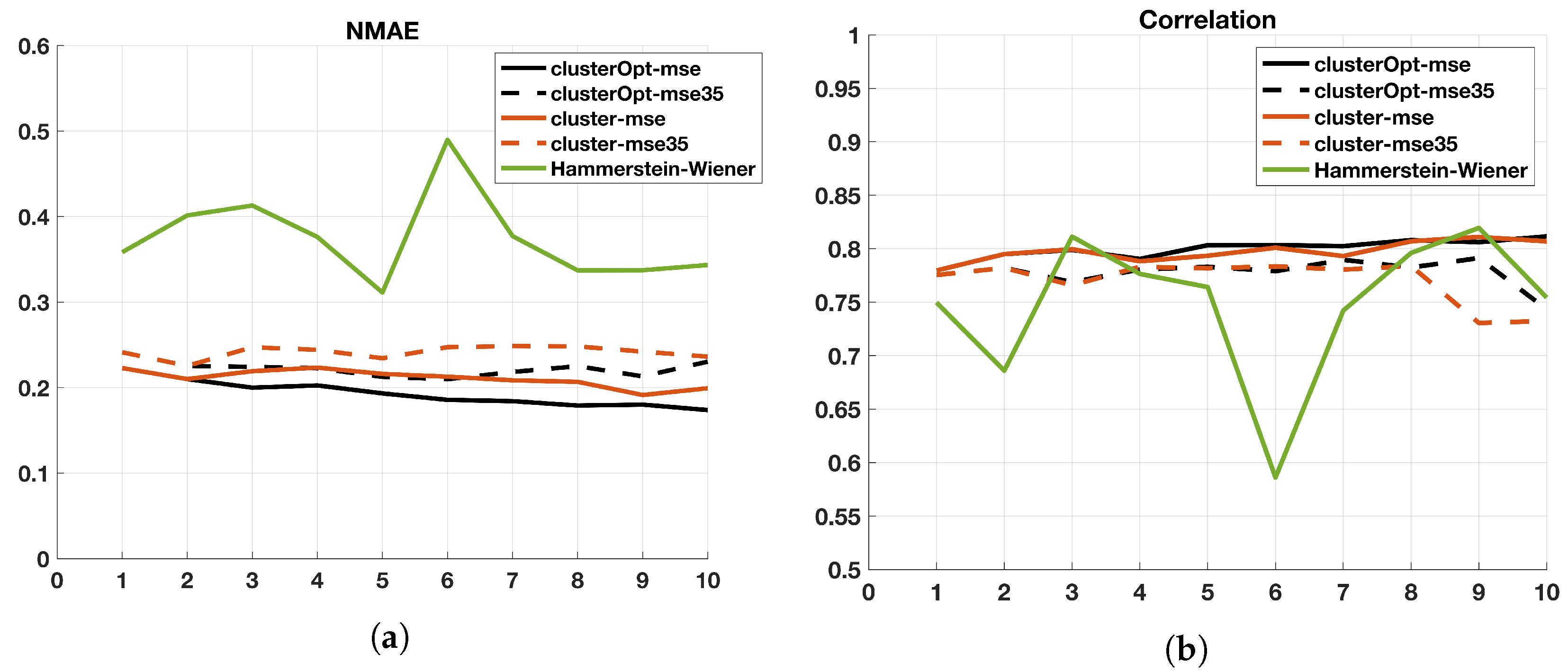
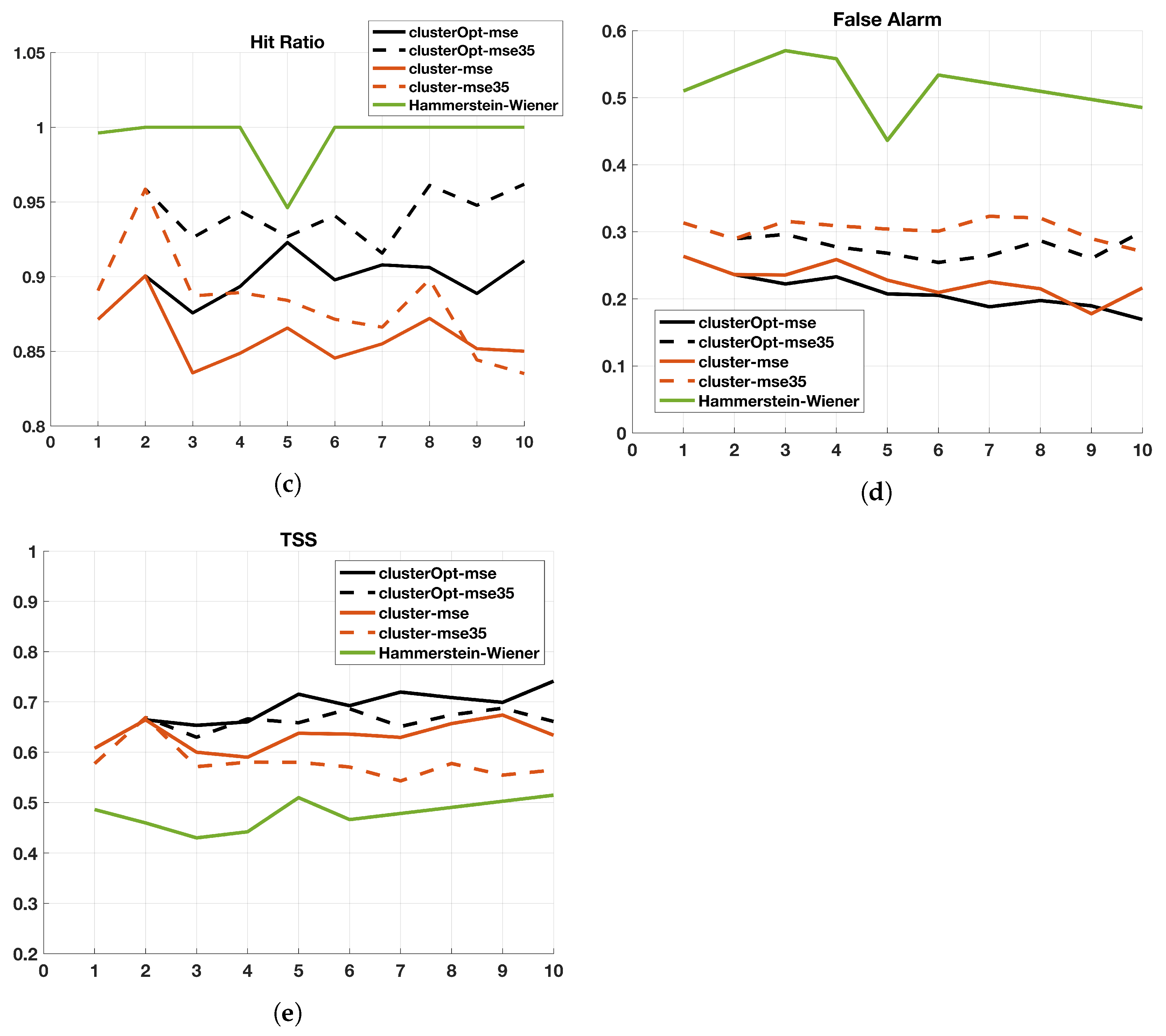
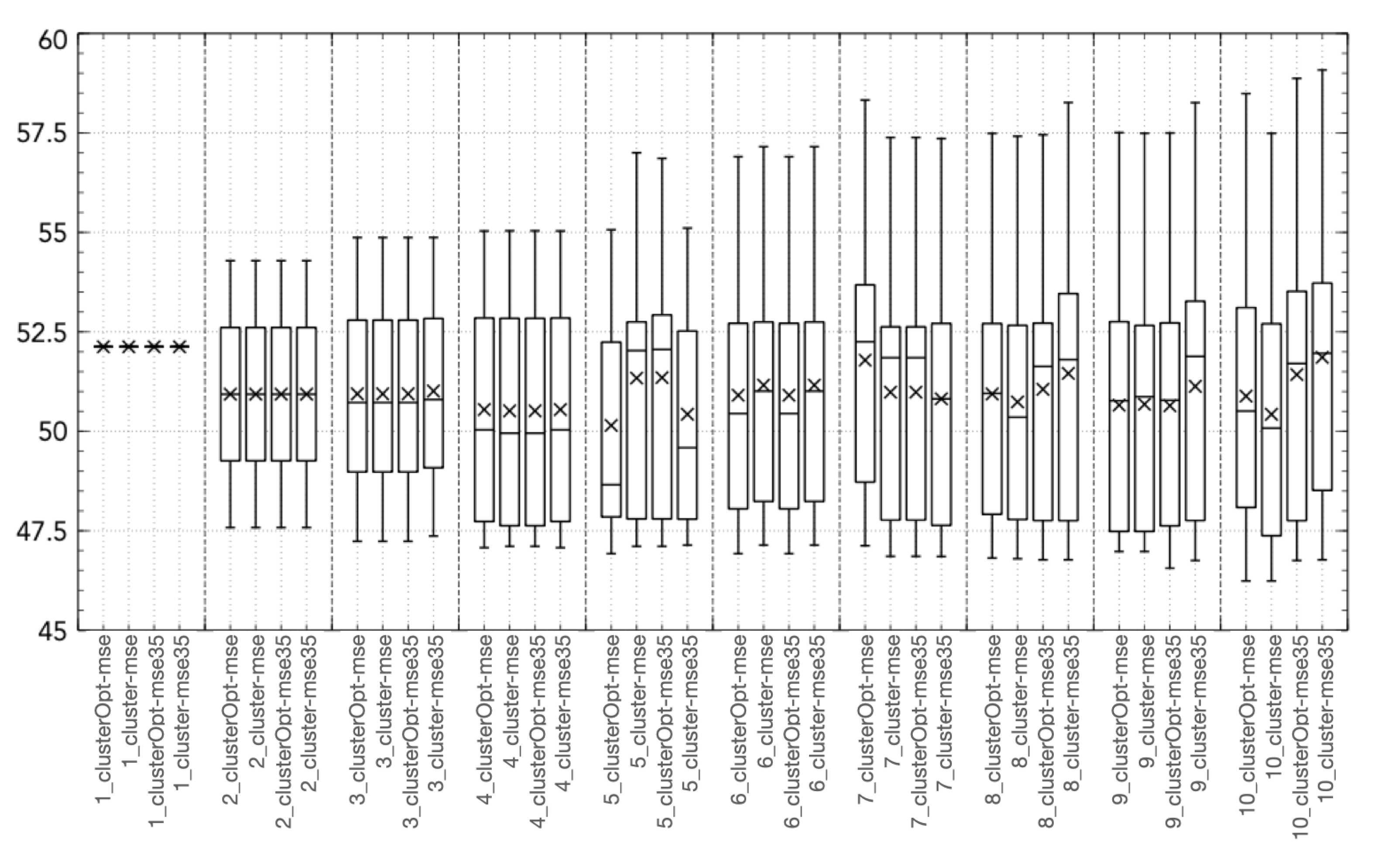
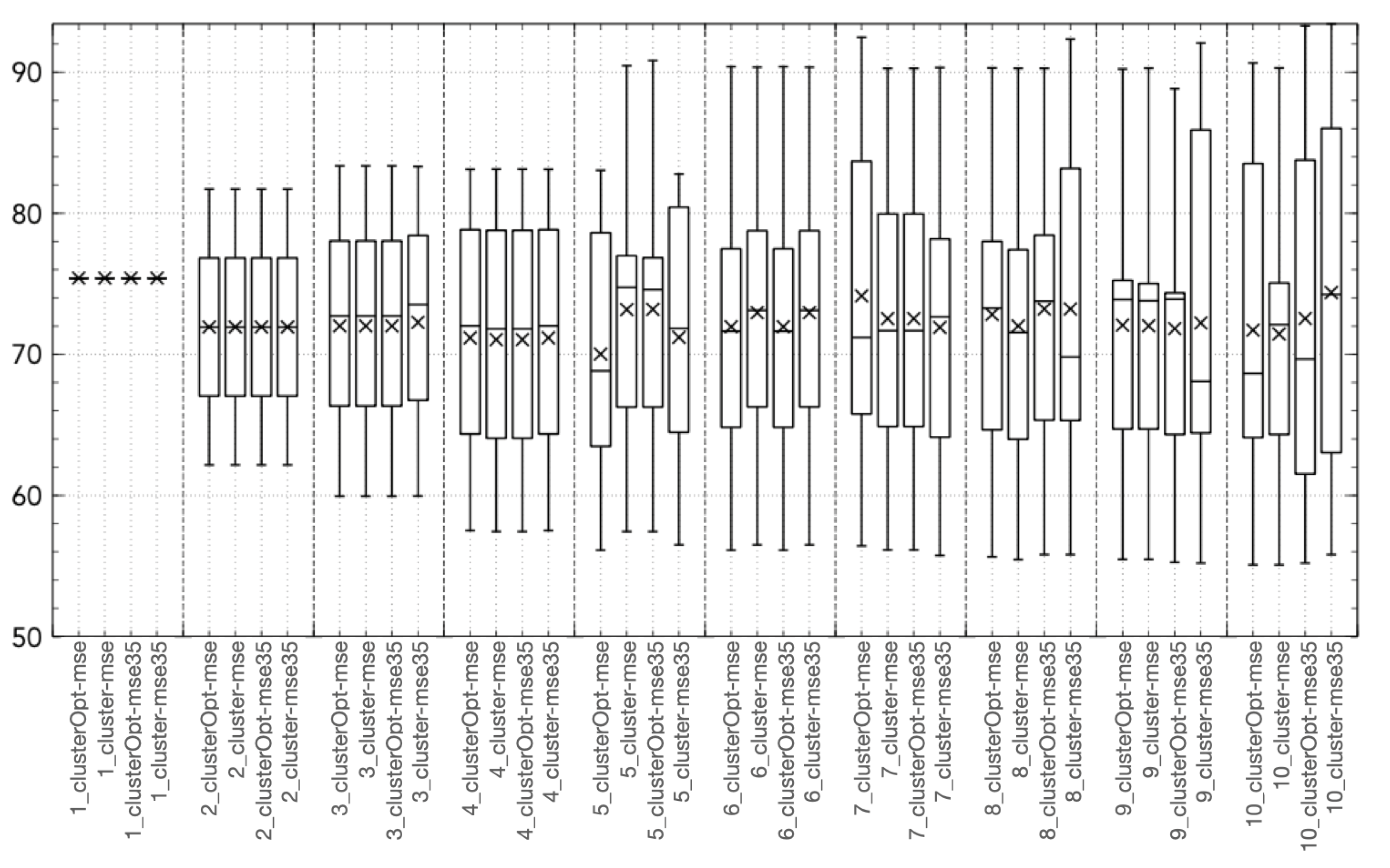
• cluster-mse: the model parameters are computed firstly applying the cluster analysis to the model input, then splitting the data on the basis of the different clusters and finally computing a model for each cluster minimizing the mean square error;
• cluster-mse35: is a variant of cluster-mse, where only the tuples with NO${}_2$ concentrations higher than 35 $\mathsf{\mu }$g/m${}^3$ are considered in the objective function. The idea is to focus only on the highest (most critical) concentration values;
• clusterOpt-mse: the model parameters are computed by the proposed methodology, thus, jointly optimizing the centroid positions and the model parameters and dynamically splitting the dataset on the basis of the distance of the input data from the optimized centroids;
• clusterOpt-mse35: is a variant of clusterOpt-mse considering only the tuples with NO${}_2$ concentrations higher than 35 $\mathsf{\mu }$g/m${}^3$ in the objective function.
• Hammerstein–Wiener: the model is a state-of-the-art Hammerstein-Wiener model [20] whose parameters are computed by means of the sequential quadratic programming algorithm presented in [26].

All the previous approaches receive as input a predefined number K of regions. To this aim, different tests have been performed, with K ranging from 1 (no clustering) to 10. Moreover, we have conducted some preliminary tests on the classic ARX model to define the $x_t$ structure, by evaluating different combinations of autoregressive ($n_a$) and exogenous ($n_l$) part orders.

The validation and comparison of the described five methods have been performed on the basis of two statistical indexes taking into account the corresponding output value $y_t$ and its average value ${\mu }_y$:

• Normalized Mean Absolute Error

  $$NMAE=\frac{{\sum }_{t=1}^N\left|(y\left(t\right)-\overline{y}\left(t\right))\right|}{{\sum }_{t=1}^{N}y\left(t\right)}$$

  (7)
• Correlation Coefficient

  $$Corr=\frac{{\sum }_{t=1}^N(y\left(t\right)-{\mu }_y)(\overline{y}\left(t\right)-{\mu }_{\overline{y}})}{\sqrt{{\sum }_{t=1}^N{(y\left(t\right)-{\mu }_y)}^2}·\sqrt{{\sum }_{t=1}^N{(\overline{y}\left(t\right)-{\mu }_{\overline{y}})}^2}}$$

  (8)

and on the basis of 3 specific indexes: the daily exceedances of the threshold of 35 $\mathsf{\mu }$g/m${}^3$ correctly reproduced (Hit Ratio), the false alarm (with the same threshold) and the True Skill Score. The last three indexes are computed through the contingency

Table 2. Contingecy table for the daily exceedances of the threshold of 35 $\mathsf{\mu }$g/m${}^3$.

		Observed Values
		≥35 $\mathsf{\mu }$g/m${}^3$	<35 $\mathsf{\mu }$g/m${}^3$
Model	≥35 $\mathsf{\mu }$g/m${}^3$	$TP$	$FP$
	<35 $\mathsf{\mu }$g/m${}^3$	$FN$	$TN$

, where TP (true positive) is the correctly reproduced exceedances, FP (false positive) is the wrong exceedances, TN (true negative) is the correctly reproduced values under the threshold and FN is the exceedances not produced by the model. The three indexes can be calculated as:

• Hit Ratio:

  $$HR=\frac{TP}{TP+FN}$$

  (9)
• False alarm fraction:

  $$FA=\frac{FP}{TP+FP}$$

  (10)
• True Skill Score:

  $$TSS=HR-FA$$

  (11)

3.1. ARX Model Validation

In this section, the validation of the classical ARX models ($K=1$) based on the order of the autoregressive ($n_a$) and exogenous ($n_l$) parts, is presented. Only the tests with $n_a=n_l,\forall l$ are shown.

Figure 1 presents the statistical and threshold indexes described before for the orders ranging from 1 to 4. As shown by the sub-figures, the impact of the order is quite limited, with a slight improvement of the statistical indexes and false alarm (NMAE, Figure 1a: from $0.227$ to $0.22$, Correlation, Figure 1b: from $0.772$ to $0.784$, false alarm, Figure 1d: from $0.285$ to $0.255$) and no impact on the exceedance fraction (Figure 1c constant around $0.86$). Finally, the true skill score (TSS, Figure 1e) highlights the trade-off between the ability to correctly reproduce the exceedances and the capability to avoid false alarms, which is stable at around 0.6. It can be stated that, even if limited, the impact is greater when the order moves from $n_a=n_l=1$ to $n_a=n_l=2$: for this reason, from now on we will only consider these two values.

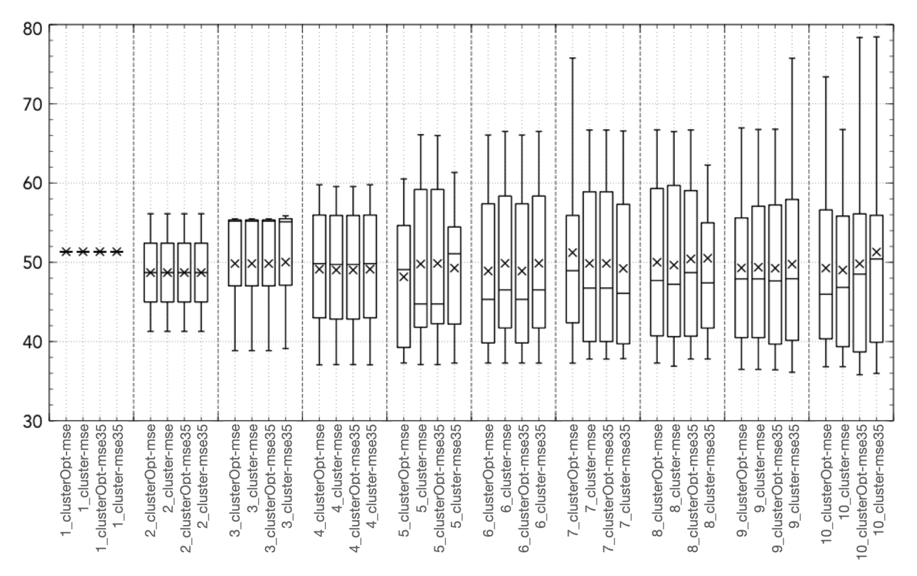
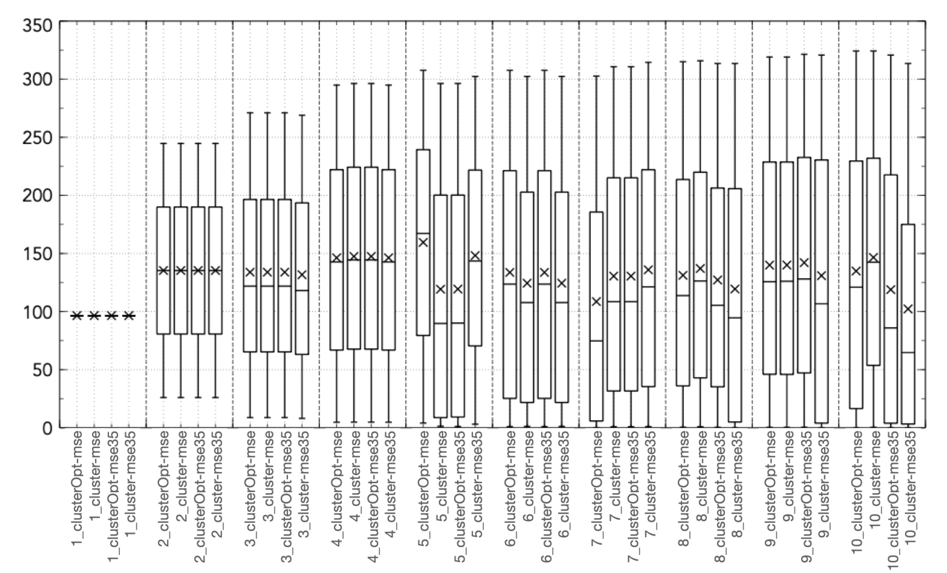
3.2. Validation and Comparison of Solution Methods

Figure 2 shows the performance in terms of the selected indexes for the tested methods when an ARX model, with $n_a=n_l=1,\forall l$ and the number of regions K ranging from 1 to 10, are set. For the Hammerstein-Wiener models, a number of the input unit and output unit equal to $n_a$ have been considered.

We start comparing the methods with the classic ARX model analyzed in Section 3.1. As far as static or optimized approaches that consider all the data in the training set (cluster-mse, clusterOpt-mse) are considered, the tests show a clear improvement, with NMAE dropping from 0.227 to 0.19, Correlation increasing from 0.77 to 0.81, Hit Ratio increasing from 0.86 to 0.88 and a quite strong improvement in false alarm, from 0.27 to 0.19. In these cases, the better performance obtained with the optimization of the centroids can be noticed for $K>2$. When testing the methods using only the values over the threshold of 35 $\mathsf{\mu }$g/m${}^3$ (cluster-mse35, clusterOpt-mse35) the behavior is less clear probably due to the effect induced by the threshold in the objective function. Moreover, as expected, the hit ratio performance are better when the tests cluster-mse35 and clusterOpt-mse35 are performed, reaching values over 0.94 and 0.99 for $K=9$, respectively. Notice that, for clusterOpt-mse and clusterOpt-mse35, the True Skill Score shows an increasing trend with values oscillating from 0.6 to around 0.7, although performance of clusterOpt-mse is better. This is due to the fact that the optimized distribution of the centroids allows ClusterOpt to define a set of dedicated models according to the different dynamics and characteristics of the system itself.

All the “cluster-based” tested approaches outperform Hammerstein–Wiener models with the same number of input/output units, with the exception of the Hit Ratio (Figure 2c). This behavior is caused by a tendency of the Hammerstein-Wiener model to overestimate the output variable, thus leading to a high value of the Hit Ratio but also of the False Alarm ratio, causing a low value of the True Skill Score. Figure 3, Figure 4, Figure 5, Figure 6 and Figure 7 show the distribution of the different coordinates of the centroids in the different tests. It can be noticed that with a low number of regions ($K\le 4$) the coordinates of the centroids identified by clusterOpt-mse and clusterOpt-mse35 are similar to the ones found by the initial clustering method used by the static approaches.

Finally, we briefly discuss the impact of the proposed solution methods when $n_a=n_l=2,\forall l$ (Figure 8). When no clustering is applied (case $K=1$), it seems that setting $n_a=n_l=2$ provides results slightly better than when $n_a=n_l=1$. When clusterOpt-mse and cluster-mse are considered, it can be noticed that, independently of the number of regions K, the methods perform better with $n_a=n_l=2$. A similar performance is not clear for the other approaches. The most important impact is related to the True Skill Score. In this case, the performance of clusterOpt-mse is better than the one provided by any other approach for $K\ge 3$, reaching values greater than 0.7 and close to 0.75 for $K=10$. Instead, the performance of the standard Hammerstein–Wiener model is quite far from that of the approaches based on clustering.

To conclude, the results confirm the ability of clusterOpt to better mimic the true output of the time series, without frequent over- or under-estimation errors, due to the use of focused models for each region and optimized centroids.

4. Conclusions and Future Works

In this paper, a data-driven piece-wise modeling is presented to simulate and predict the concentration of nitrogen oxides over the municipality of Milan, a heavily polluted city in the north of Italy. The methodology is based on the identification of a model from daily measured concentrations, meteorological variables, and emission levels estimated from results presented in special emission databases. To tackle this complex problem, we propose a new approach that involves the joint optimization of clustering and model parameters identification while minimizing the simulation error on the real case data. The methodology has been compared with two state-of-the-art approaches based on a two-step, cluster-based algorithm and on Hammerstein–Wiener models. The results show that the devised approach ensures better performance with respect to these two methods, both in terms of statistical indexes (correlation, normalized mean absolute error) and in terms of problem-specific metrics (hit ratio, false alarm) due to the capability of the identification phase to identify models representing the different model behavior through a jointly optimized methodology. Although, the goal of the work, intended as the identification of models allowing good performance in the representation of complex phenomena with limited complexity, can be considered as achieved, a detailed comparison with fully nonlinear models (artificial neural network and support vector machine to name a few) will be performed in the next future. Moreover, this work can be considered the starting point needed for the development and implementation of an emission control problem that aims at selecting optimal actions to reduce the impact of pollutants in the atmosphere.

References

1. Pope, C., III; Dockery, D.; Spengler, J.; Raizenne, M. Respiratory health and PM10 pollution: A daily time series analysis. Am. Rev. Respir. Dis. 1991, 144, 668–674. [Google Scholar] [CrossRef] [PubMed]
2. Pope, C., III; Dockery, D. Acute health effects of PM10 pollution on symptomatic and asymptomatic children. Am. Rev. Respir. Dis. 1992, 145, 1123–1128. [Google Scholar] [CrossRef] [PubMed]
3. Manerba, D.; Mansini, R.; Zanotti, R. Attended Home Delivery: Reducing last-mile environmental impact by changing customer habits. IFAC-PapersOnLine 2018, 51, 55–60. [Google Scholar] [CrossRef]
4. Bonomi, V.; Mansini, R.; Zanotti, R. Last Mile Delivery with Parcel Lockers: Evaluating the environmental impact of eco-conscious consumer behavior. IFAC-PapersOnLine 2022, 55, 72–77. [Google Scholar] [CrossRef]
5. Miranda, A.; Silveira, C.; Ferreira, J.; Monteiro, A.; Lopes, D.; Relvas, H.; Borrego, C.; Roebeling, P. Current air quality plans in Europe designed to support air quality management policies. Atmos. Pollut. Res. 2015, 6, 434–443. [Google Scholar] [CrossRef]
6. Carnevale, C.; Sangiorgi, L.; De Angelis, E.; Mansini, R.; Volta, M. A System of Systems for the Optimal Allocation of Pollutant Monitoring Sensors. IEEE Syst. J. 2021, 1–8. [Google Scholar] [CrossRef]
7. Carnevale, C.; Finzi, G.; Pederzoli, A.; Pisoni, E.; Thunis, P.; Turrini, E.; Volta, M. A methodology for the evaluation of re-analyzed PM10 concentration fields: A case study over the PO Valley. Air Qual. Atmos. Health 2015, 8, 533–544. [Google Scholar] [CrossRef]
8. Candiani, G.; Carnevale, C.; Finzi, G.; Pison, E.; Volta, M. A comparison of reanalysis techniques: Applying optimal interpolation and Ensemble Kalman Filtering to improve air quality monitoring at mesoscale. Sci. Total. Environ. 2013, 458–460, 7–14. [Google Scholar] [CrossRef]
9. San José, R.; Pérez, J.L.; Morant, J.L.; González, R.M. European operational air quality forecasting system by using MM5–CMAQ–EMIMO tool. Simul. Model. Pract. Theory 2008, 16, 1534–1540. [Google Scholar] [CrossRef]
10. Manders, A.; Schaap, M.; Hoogerbrugge, R. Testing the capability of the chemistry transport model LOTOS-EUROS to forecast PM10 levels in the Netherlands. Atmos. Environ. 2009, 43, 4050–4059. [Google Scholar] [CrossRef]
11. Samaké, A.; Mahamane, A.; Alassane, M.; Diallo, O. A Mathematical and Numerical Framework for Traffic-Induced Air Pollution Simulation in Bamako. Computation 2022, 10, 76. [Google Scholar] [CrossRef]
12. Carnevale, C.; Finzi, G.; Guariso, G.; Pisoni, E.; Volta, M. Surrogate models to compute optimal air quality planning policies at a regional scale. Environ. Model. Softw. 2012, 34, 44–50. [Google Scholar] [CrossRef]
13. Carnevale, C.; Finzi, G.; Pederzoli, A.; Turrini, E.; Volta, M. Lazy Learning based surrogate models for air quality planning. Environ. Model. Softw. 2016, 83, 47–57. [Google Scholar] [CrossRef]
14. Rahman, Z.A.S.A.; Jasim, B.H.; Al-Yasir, Y.I.A.; Abd-Alhameed, R.A.; Alhasnawi, B.N. A New No Equilibrium Fractional Order Chaotic System, Dynamical Investigation, Synchronization, and Its Digital Implementation. Inventions 2021, 6, 49. [Google Scholar] [CrossRef]
15. Rahman, Z.A.S.A.; Jasim, B.H.; Al-Yasir, Y.I.A.; Hu, Y.F.; Abd-Alhameed, R.A.; Alhasnawi, B.N. A New Fractional-Order Chaotic System with Its Analysis, Synchronization, and Circuit Realization for Secure Communication Applications. Mathematics 2021, 9, 2593. [Google Scholar] [CrossRef]
16. Carnevale, C.; Finzi, G.; Pisoni, E.; Singh, V.; Volta, M. An integrated air quality forecast system for a metropolitan area. J. Environ. Monit. 2011, 13, 3437–3447. [Google Scholar] [CrossRef]
17. Wu, Y.; Ding, Y.; Feng, J. SMOTE-Boost-based sparse Bayesian model for flood prediction. EURASIP J. Wirel. Commun. Netw. 2020, 2020, 78. [Google Scholar] [CrossRef]
18. Wu, Y.; Han, P.; Zheng, Z. Instant water body variation detection via analysis on remote sensing imagery. J. Real-Time Image Process. 2021, 18, 1577–1590. [Google Scholar] [CrossRef]
19. Carnevale, C.; Turrini, E.; Zeziola, R.; De Angelis, E.; Volta, M. A Wavenet-Based Virtual Sensor for PM10 Monitoring. Electronics 2021, 10, 2111. [Google Scholar] [CrossRef]
20. Dolanc, G.; Strmčnik, S. Identification of nonlinear systems using a piecewise-linear Hammerstein model. Syst. Control Lett. 2005, 54, 145–158. [Google Scholar] [CrossRef]
21. Hadid, B.; Duviella, E.; Lecoeuche, S. Data-driven modeling for river flood forecasting based on a piecewise linear ARX system identification. J. Process Control 2020, 86, 44–56. [Google Scholar] [CrossRef]
22. Ipanaqué, W.; Manrique, J. Identification and Control of pH using Optimal Piecewise Linear Wiener Model. IFAC Proc. Vol. 2011, 44, 12301–12306. [Google Scholar] [CrossRef]
23. Westra, R.L.; Ralf, M.P.; Peeters, L. Identification of Piecewise Linear Models of Complex Dynamical Systems. IFAC Proc. Vol. 2011, 44, 14863–14868. [Google Scholar] [CrossRef]
24. Yang, X.; Yang, H.; Zhang, F.; Zhang, L.; Fan, X.; Ye, Q.; Fu, L. Piecewise Linear Regression Based on Plane Clustering. IEEE Access 2019, 7, 29845–29855. [Google Scholar] [CrossRef]
25. Liu, J.; Xu, Z.; Zhao, J.; Shao, Z. Identification of piecewise affine model for batch processes based on constrained clustering technique. Chem. Eng. Res. Des. 2022, 181, 278–286. [Google Scholar] [CrossRef]
26. Nocedal, J.; Wright, S.J. Numerical Optimization, 2nd ed.; Springer: New York, NY, USA, 2006. [Google Scholar]
27. Li, Y.; Wu, H. A Clustering Method Based on K-Means Algorithm. Phys. Procedia 2012, 25, 1104–1109. [Google Scholar] [CrossRef]
28. Zhang, J.; Chin, K.S.; awryńczuk, M. Nonlinear model predictive control based on piecewise linear Hammerstein models. Nonlinear Dyn. 2018, 92, 1001–1021. [Google Scholar] [CrossRef]
29. Lassoued, Z.; Abderrahim, K. Identification and control of nonlinear systems using PieceWise Auto-Regressive eXogenous models. Trans. Inst. Meas. Control 2019, 41, 4050–4062. [Google Scholar] [CrossRef]
30. Schittkowski, K. NLQPL: A FORTRAN-Subroutine Solving Constrained Nonlinear Programming Problems. Ann. Oper. Res. 1985, 5, 485–500. [Google Scholar] [CrossRef]
31. INEMAR—Arpa Lombardia. INEMAR. Emission Inventory: 2014 Emission in Region Lombardy—Public Review; Technical Report; ARPA Lombardia Settore Aria: Milano, Italy, 2017. [Google Scholar]
Figure 1. Index values (ordinate axis) of ARX model for ( K = 1 ) with n a = n l = 1 4 (abscissa axis). (a) Normalized Mean Absolute Error (NMAE); (b) Correlation Coefficient; (c) Hit Ratio; (d) False Alarm; (e) True Skill Score (TSS).
Electronics 11 02770 g001
Figure 2. Index values (ordinate axis) of the 5 compared methods for K = 1 10 (abscissa axis) when n a = n l = 1 . (a) Normalized Mean Absolute Error (NMAE); (b) Correlation Coefficient; (c) Hit Ratio; (d) False Alarm; (e) True Skill Score (TSS).
Electronics 11 02770 g002
Figure 3. Boxplot of coordinate 1 ( y ( t 1 ) , NO 2 concentration at time t 1 ) of the centroid [ μ g/m 3 ].
Electronics 11 02770 g003
Figure 4. Boxplot of coordinate 2 ( u 1 ( t ) , NO x emissions at time t) of the centroid [kg/d/m 2 ].
Electronics 11 02770 g004
Figure 5. Boxplot of coordinate 3 ( u 2 ( t ) , daily mean temperature at time t) of the centroid [ C ] .
Electronics 11 02770 g005
Figure 6. Boxplot of coordinate 4 ( u 3 ( t ) , daily mean humidity at time t) of the centroid [ % ] .
Electronics 11 02770 g006
Figure 7. Boxplot of coordinate 5 ( u 2 ( t ) , daily solar radiation at time t) of the centroid [kw/h].
Electronics 11 02770 g007
Figure 8. Index values (ordinate axis) of the 5 compared methods for K = 1 10 (abscissa axis) when n a = n l = 2 . (a) Normalized Mean Absolute Error (NMAE); (b) Correlation Coefficient; (c) Hit Ratio; (d) False Alarm; (e) True Skill Score (TSS).
Electronics 11 02770 g008aElectronics 11 02770 g008b