Deep LSTM Model for Diabetes Prediction with Class Balancing by SMOTE

Abstract

Diabetes is an acute disease that happens when the pancreas cannot produce enough insulin. It can be fatal if undiagnosed and untreated. If diabetes is revealed early enough, it is possible, with adequate treatment, to live a healthy life. Recently, researchers have applied artificial intelligence techniques to the forecasting of diabetes. As a result, a new SMOTE-based deep LSTM system was developed to detect diabetes early. This strategy handles class imbalance in the diabetes dataset, and its prediction accuracy is measured. This article details investigations of CNN, CNN-LSTM, ConvLSTM, and deep 1D-convolutional neural network (DCNN) techniques and proposed a SMOTE-based deep LSTM method for diabetes prediction. Furthermore, the suggested model is analyzed towards machine-learning, and deep-learning approaches. The proposed model’s accuracy was measured against the diabetes dataset and the proposed method achieved the highest prediction accuracy of 99.64%. These results suggest that, based on classification accuracy, this method outperforms other methods. The recommendation is to use this classifier for diabetic patients’ clinical analysis.

1. Introduction

Diabetes is a chronic illness that occurs when blood sugar is not adequately processed. Over time, it can affect many organs, causing long-term damage and malfunction. The diabetic disease [1] can cause serious complications, such as nervous-system damage, heart attacks, kidney failure, and stroke. Hyperglycemia is a condition in which the body’s glucose levels are too high, resulting in anomalies in the cardiovascular system and major difficulties with the functioning of numerous human organs such as the eyes, kidneys, and nerves. This research attempted to concentrate on the finding of diabetes [2,3] using the Pima Indian Diabetes Dataset (PIDD) [4]. This is available in the UCI (the University of California at Irvine) Repository. Class imbalance is a situation in which the number of instances in all the classes is not equal. The classes with most instances are referred to as the majority classes, and the classes with fewer instances are referred to as the minority classes. The imbalance of any dataset can be easily measured by using the class-imbalance ratio (CIR), which is defined as a ratio between the number of minority instances and the number of majority instances. The class imbalance in the dataset degrades the performance of the machine-learning algorithm. As the machine-learning model is trained with majority-class-label instances, this leads to a lack of recognition of minority-class instances. This problem is termed overfitting. The solution is to make the imbalanced dataset into a balanced dataset before training starts. Data augmentation provides augmented data to handle the imbalanced data before the training process. Random sampling is the most straightforward data augmentation technique. In this technique, the samples are generated randomly from the minority-class instances. Undersampling and oversampling are the two popular random sampling techniques. The undersampling method removes the instances randomly from the majority-class instances. Hence the number of instances in both majority- and minority-class labels become equal. The limitation of this approach is data loss. The oversampling method duplicates the instances taken from the minority class to make the minority class similar in size to the majority class. Since the same instances are repeated, the classifier’s accuracy is improved compared to the performance of the classifier trained with an imbalanced dataset. On the other hand, synthetic sample generation-based oversampling is called the synthetic minority oversampling Technique (SMOTE). It generates samples synthetically between each minority instance and its neighbors. Deep-learning-based classifiers perform better than machine-learning classifiers. Long short-term memory (LSTM) is a popular recurrent neural network (RNN) that can be trained with many layers to improve model training accuracy.

For diabetes prognosis, the SMOTE sampling strategy is included in time series forecasting for class imbalance. The two-class neural network employs Pima Indian data for diabetes prediction [5]. The authors pre-processed the data, who normalized the attribute using the standardization technique. They also used correlation to extract the essential features. On the other hand, the authors did not mention these discriminatory characteristics. Compared to the accuracy acquired from earlier studies, the model attained the best accuracy of 83.3% after being divided into training data of 314 instances and test data of 78 instances. Deep learning is a subset of machine learning and plays a promising role in the field of time-series prediction. Class imbalance is a challenging issue in medical data including the PIDD. A 1D-convolutional neural network (DCNN) method [6] handled the class-imbalanced Pima Indian diabetic data set and classified the patient as diabetic or non-diabetic, and its classification accuracy was 86.29%. Hence another deep-learning model was built in this work with SMOTE to convert imbalance data into balanced data before the classification of diabetes or not. The initial class-imbalanced data set was processed with the synthetic minority oversampling technique (SMOTE) method [7]. The proposed method, SMOTE-based deep LSTM, is a fusion of SMOTE and LSTM layers for diabetes prediction. The novelty of this paper is class-imbalance learning and prediction using SMOTE-based deep LSTM. Various comparative evaluations were conducted to determine where our model performs better and where it performs worse. We also fine-tuned many factors in our model to determine the best configuration when the model is most accurate. We compared our model’s performance with various benchmark models.

The paper is comprised of the following sections: Section 1 presents the aims of the work. Section 2 précises the existing works on diabetes prediction. The proposed SMOTE-based deep-learning model is described in Section 3. The experimental setup, performance indicators, and results and comparisons are described in Section 4. Finally, Section 5 concludes the paper and presents future work.

2. Related Works

Many real-world applications of the class-imbalanced problem exist, including fraud detection [8] and medical diagnostics [9,10,11]. In classification, unbalanced learning poses a problem. The synthetic minority oversampling technique over-samples the minority class. It is a type of data augmentation in which current samples are used to create new samples. It establishes lines connecting similar samples in the minority class. On these lines, new sample points are added. More specifically, a random sample is selected, and then the K-nearest neighbor (KNN) algorithm is used to choose neighbors to whom lines are drawn. With this procedure, many synthetic samples are created as needed, which means that the SMOTE method is suitable for data sets of all sizes. Class-wise k-Nearest Neighbor (CkNN) is another method for diabetes classification [12]. Cascade learning system mitigates the issues in identifying the diabetic disease [13]. It consists of Generalized Discriminant Analysis and Least Square Support Vector Machine for classification. It provides a promising accuracy of 82.05%. Hybrid neural network is another work that combines Artificial Neural Network (ANN) [14] and Fuzzy Neural Network (FNN) [15]. General regression neural network is also used for diabetic recognition using PIDD [16]. The performance is compared by various training algorithms.

Deep learning mitigates many issues in learning the features from diabetic dataset and makes the classification easier [17,18]. The performance of the hybrid model is measured by Pima Indians diabetes and Cleveland heart disease datasets. The deep belief network [19] was applied over a diabetes dataset for diabetic prediction and achieved a prediction accuracy of 81.20%. MLP based logistic regression is used for continuous glucose monitoring (CGM) and identifies diabetic or not [20]. The data set contained nine individuals of CGM data for 10,800 days and a total of 97,200 days was simulated. For cross-validation, the data set was separated into training, validation, and testing data. Three patients were chosen for testing, and six were chosen for training and validation and the accuracy was 77.5%. A deep-learning stacked autoencoder with a deep neural network used L-BFGS and performed optimization with classification accuracy on PIDD was 77.09% [21]. Three distinct DL algorithms are tested on an Australian hospital’s manually collected data [22]. The data set consisted of 12,000 samples (patients) with a male-to-female ratio of 55.5%. Some pre-processing techniques were used to limit the observations to 7191. The data set was divided into two-thirds for training, one-sixth for validation, and one-sixth for testing for validation. The performance of models such as long short-term memory (LTSM), Markov, and recurrent neural networks (RNN) was compared using the precision value. Long short-term memory achieved a precision value of 59.6%. The recurrent neural network that predicts the type of diabetes from all eight attributes [23]. The data set was divided into 80:20 for training and test sets to validate the work. Type 1 diabetes was correctly predicted 78% of the time, whereas type 2 diabetes was correctly predicted 81% of the time. A few researchers have proposed a deep-learning-based big medical data analytics model using a deep-belief network for diabetes classification from few factors selected from 50,000 diabetic data sets. The accuracy was 81.20%. Multilayer neural network (MLNN) is trained by LM algorithm for diabetic prediction using PIDD and compared with probabilistic neural network (PNN) [24]. This method is evaluated by 10-fold cross validation.

Moth-flame-based crow search algorithm (MFCSA) is popularly used for diabetes detection [25] and glucose-level prediction [17]. It is a hybrid approach that selects optimal features followed by classification. The advantage of this approach is avoiding redundant attributes. The ensemble classifier uses t-distributed stochastic neighbor-embedding technique for type 2 diabetes prediction [18]. It also uses dimensionality reduction. This approach solves the overfitting problem. The enhanced and adaptive-genetic algorithm-multilayer perceptron (EAGA-MLP) generates an optimized dataset by optimizing the attributes followed by a classification process [1].

Long short-term memory is postulated for time-series prediction [26]. In time-series forecasting, LSTM is a type of recurrent neural network. There are three layers called the input, hidden, and output layers. Memory cells in the hidden layer have three gates that update the state of the cell. Unlike RNNs, the vanishing gradient problem does not exist in LSTM networks. This is essential for diabetes prediction since old information is handled in the network [27]. In fact, three-dimensional input in the form of samples, time steps, and features is supported by LSTM. One or more samples may be included in a batch. If we are dealing with text at the sentence level (that is, one sentence at a time) in natural-language processing, our sample size will be one. The number of times the input is given to the model can be thought of as the time step.

The limitations of previous work are class-imbalance problems, optimized dataset generation, redundant attribute reduction and dimensionality reduction. The contributions of the proposed method are given as follows:

• Designing a deep-learning classifier for diabetic recognition;
• Incorporating SMOTE to treat the class-imbalance problem and improve the accuracy of the deep-learning classifier.

3. Diabetes Prediction

Deep-learning techniques were used in this work for predicting the diabetic illness. The traditional machine-learning procedures do not need to be explicitly described in DL networks. The main task of deep learning is self-learning the hidden patterns in the data. This section describes the various deep-learning methods used in this work, such as CNN [28], CNN-LSTM [29], ConvLSTM [30], and DCNN [6] for comparison with the proposed method of SMOTE-based deep LSTM. The convolutional neural network is popular in numerous applications [28] such as medical image analysis and object detection and CNNs have demonstrated good performance. The convolutional neural network takes local features that flow through lower layers for extracting complex features. The convolutional layer comprises a set of kernels that are used to calculate a tensor of feature mappings. The kernels use “stride(s)” to convolve an entire input so that the dimensions of an output volume become integers [29]. After the convolutional layer is utilized to perform the striding process, the dimensions of an input volume shrink. As a result, an input which has undergone zero padding in order to hold the size of an input features zero padding [30] is required. The convolutional layer operation is given in Equation (1):

$$F\left(i,j\right)={\displaystyle \sum }{\displaystyle \sum }I\left(i+m,j+n\right)K\left(m,n\right)$$

(1)

where $I$ denotes input matrix, $K$ represents a kernel with $m\times n$ size, and $F$ denotes the result of feature map. The convolution operation $i\ast K$ takes place in the convolutional layer. The activation function rectified linear unit (ReLU) is used for generating nonlinearity in feature maps and it is defined in Equation (2).

$$f\left(x\right)=\max \left(0, x\right)$$

(2)

The pooling layer [31] applies down-sampling on the input in order to reduce the number of parameters. Max pooling selects the maximum value from the input. Finally, the fully connected (FC) layer acts as a classifier [32].

Hochreiter and Schmidhuber [28] invented long short-term memory which can transfer data between sequences. In LSTM, every computational step considers not just the current input at time t, but also what has been learned from past inputs [33]. The Pima Indian Diabetes Dataset was used to estimate diabetes using a combination of LSTM and CNN methods. To match the three-dimensional input requirements of the Keras sequential model, the data was first scaled, balanced, and reshaped. For a multivariate model, the input shape would be 24 time steps with 9 features. Within the convolutional layer, the sequence is not divided into multiple subsequences but the time steps are kept at 24 instead and the kernel size is three. The dense layer is made up of 24 neurons that generate 24 output numbers. The following Equation (3) shows how to extract features from the altered data using CNN. The featured LSTM extracted are expressed in Equation (4).

$$CN{N}_{features}=CNN(Reshape\left(x\left(t\right)\right)$$

(3)

$$LST{M}_{features}=LSTM\left(CN{N}_{features}\right)$$

(4)

Another network structure is ConvLSTM. This hybrid network has convolution1D and max-pooling layers. Equation (5) depicts the convolution process. The max-pooling 1D layer’s output is sent into the next LSTM layer.

$$y_i=CNN\left(x_i\right)$$

(5)

where $x_i$ is the CNN network’s initial input vector with target label, $y_i$ is the network outcome, which is given to the next LSTM module, and $x_i,$ the CNN’s max-pooling process, produces a feature vector. It is fed into the LSTM which uses it to learn the long-term temporal dependencies. The LSTM works in a following way: The length of input $x=\left(x_1,x_2,\dots x_{T-1},x_T\right)$ is fed to LSTM structure and the output sequence $o=\left(o_1,o_2,\dots o_{T-1},o_T\right)$. Its multiplicative units are found iteratively from $t=1 to T$ in the LSTM architecture’s hidden layer. Equations (6) to (10) can be used to illustrate the sequence of operations that occur in LSTMs at each time step $x_t,h_{t-1},c{l}_{t-1}\to h_t,\mathrm{and} c{l}_t$.

$$i{n}_t=\sigma \left(w_{xin}{x}_t+w_{hin}{h}_{t-1}+w_{clin}c{l}_{t-1}+b_{in}\right)$$

(6)

$$f{r}_1=\sigma \left(w_{xfr}{x}_t+w_{hfr}{h}_{t-1}+w_{clfr}c{l}_{t-1}+b_{fr}\right)$$

(7)

$$c{l}_t=f{r}_t· c{l}_{t-1}+i{n}_t ·\mathrm{sigmoid}\left(w_{xcl}{x}_t+w_{hcl}{h}_{t-1}+b_{cl}\right)$$

(8)

$$o{t}_t=\sigma \left(w_{xot}{x}_t+w_{hot}{h}_{t-1}+w_{clot}c{l}_t+b_{ot}\right)$$

(9)

$$h_t=o{t}_t·\mathrm{sigmoid}\left(c{l}_t\right)$$

(10)

The DCNN method accepts the preprocessed data from the Tukey method and SMOTE which is given in Equation (11). In this work the Pima Indian Diabetes Dataset was focused on diabetic prediction. The balanced data set is divided into training and testing data in a 70:30 ratio. The series of deep 1D-CNN layers involved performs 1D convolution for diabetic classification.

$$Balanced=SMOTE\left(Tukey\left(Dataset\right)\right)$$

(11)

3.1. Data Set

The Pima Indian Data Set was chosen because of the top occurrence of type 2 diabetes among Pima Native Americans living in southern Arizona. Because of a genetic propensity, this group has, for years, had a low-carbohydrate diet [31]. There was an abrupt change from traditional crops to managed foods, and the Pima population has developed a high prevalence of diabetes in recent years. The Pima Indian Diabetes Dataset includes details about 768 patients living in USA. This data set has eight numeric attributes and contains details of female patients with a minimum age of 21 years. The target has the values to indicate whether the patient is diabetic or not. The complete details of the data set are given in

Table 1. Attributes of the PIDD.

Attribute	Range	Average
Age	21 to 81	33
Pregnancies	0 to 17	4
Glucose (2 h)	0 to 199	121
Blood pressure (mm Hg)	0 to 122	69
Skin thickness (mm)	0 to 99	21
Insulin (mu U/mL)	0 to 846	80
BMI (Kg/m2)	0 to 67.1	32
Diabetes pedigree function	0.078 to 2.42	0.47
Outcome	either 0 or 1	-

. The data set is available on the Kaggle platform [4].

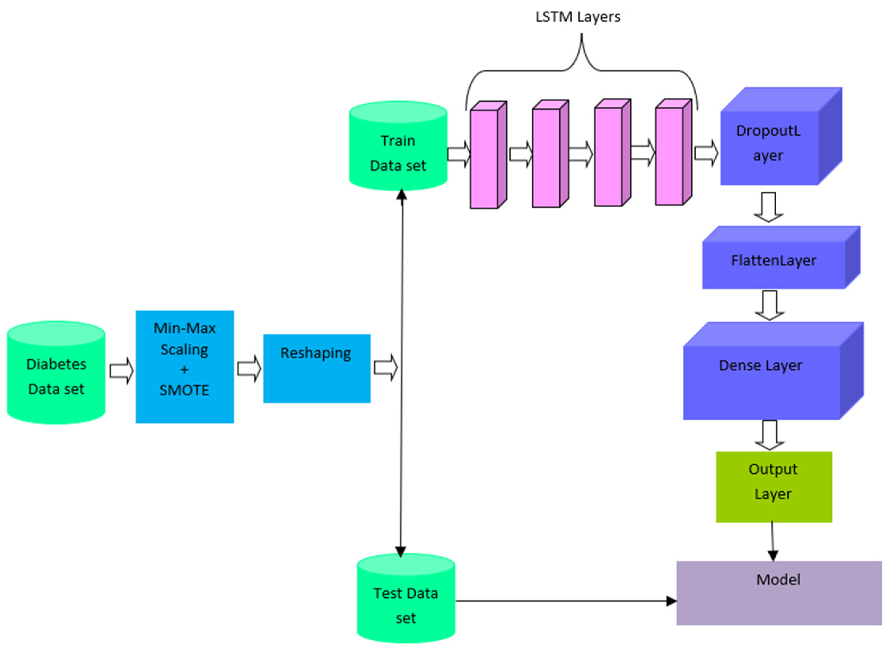
3.2. SMOTE-Based Deep LSTM for Diabetes Prediction

The challenge is to achieve diabetic classification, with good classifier performance, from a class-imbalance problem. The proposed SMOTE-based deep LSTM architecture overcomes these challenges.

3.2.1. Data Preprocessing

As a first step, the missing values are handled. Missing values are common in any healthcare data set. Compared to other methods, the Tukey method is a popular outlier-detection method which handles missing values in many applications. The normalization of the data set is performed by using the min-max transformation method. This normalizes the attributes from one range of values to a new range of values. The min-max normalization formula is given in Equation (12).

$$x^{\prime }=\left(x_{max}-x_{min}\right)\times \frac{\left(x_i-x_{min}\right)}{\left(x_{max}-x_{min}\right)}+x_{min}$$

(12)

where $x_i$ represents each instance of input, $x^{\prime }$ represents scaled input data and $x_{max}, x_{min}$ denotes maximum and minimum value in the input $x$. This preserves the relationship between data.

3.2.2. Class-Imbalance Processing

The robustness and generalization performance of classifiers trained on imbalanced data sets should be reduced. This is a key problem of machine learning. The SMOTE method handles imbalanced data and as all the columns in the PIDD are numerical, it is acceptable for SMOTE. SMOTE’s core idea is to insert new samples at random between minority samples and their neighbors. The K-nearest neighbors is first examined from the samples of minority-class samples. Assuming that the data set’s sampling magnification is N, there are N samples from K-NN and K > N. The interpolation formula of SMOTE is in Equation (13).

$$S_i=X+rand\left(0,1\right)\times \left(y_i-X\right)$$

(13)

where $X$ denotes a data sample in minority-class samples, $rand\left(0,1\right)$ denotes a random number from the interval (0,1), $y_i$ represents the $i^{th}$ nearest neighbors, and $S_i$ is the interpolated sample.

3.2.3. Reshaping

For LSTM, the input data needs to be time-series data. Hence, here the balanced data set needs to be reshaped into 3D data. The input data set consists of nine attributes represented as $x_i$ in Equation (14). Further, the raw balanced samples are reshaped into 3D data as in Equation (15), which satisfies the input requirements for deep-learning model.

$$input={\displaystyle \sum }_{i=1}^8{x}_i$$

(14)

$$Tenso{r}_{input}=reshape\left(x_i\right)$$

(15)

3.2.4. Deep LSTM

The novelty of the proposed work is its ability to handle unbalanced data in diabetes prediction. SMOTE is a common oversampling strategy for dealing with class-imbalanced data sets that produces new minority-class samples. After oversampling, the balanced data is reshaped into 3D data. Then the data is divided into training and testing data. Figure 1 shows the architecture of SMOTE-based deep LSTM. SMOTE is based on selecting the number of nearest neighbors, K = 5. LSTM accepts input data to be a 3D tensor such as batch size, timesteps, and features. The proposed model includes four LSTM layers. The overfitting problem is solved by using a dropout hyperparameter [5]. Adaptive moment estimation (Adam) is used for optimization.

Table 2. Layer-wise training detail of SMOTE-based deep LSTM model.

Layer	Input	Output	Parameter
SMOTE	#Minority instances = 268 # Majority instances = 500	# Minority instances = 500 # Majority instances = 500	K = 5
LSTM1	# Training data = 700 [20 × 35]	(20 × 30)	Hidden units = 96 Learning rate = 0.005 Batch size = 20 Loss = MSE Optimizer = Adam Dropout = 0.5 # Epochs = 417 Return Sequences = true
LSTM2	# Training data = 600 (20 × 30)	(20 × 25)	Hidden units = 96 Learning rate = 0.005 Batch size = 20 Loss = MSE Optimizer = Adam Dropout = 0.5 # Epochs = 351 Return Sequences = true
LSTM3	# Training data = 500 (20 × 25)	(20 × 20)	Hidden units = 96 Learning rate = 0.005 Batch size = 20 Loss = MSE Optimizer = Adam Dropout = 0.5 # Epochs = 325 Return Sequences = true
LSTM4	# Training data = 400 (20 × 20)	(20 × 15)	Hidden units = 96 Learning rate = 0.005 Batch size = 20 Loss = MSE Optimizer = Adam Dropout = 0.5 # Epochs = 200 Return Sequences = true
Flatten	(20 × 15)	300	-
FC	300	-	Number of neurons = 15 Activation = sigmoid
Output	-	-	Activation = sigmoid

^# Represents the count.

shows the detailed layer-wise training process of the SMOTE-based deep LSTM model.

3.2.5. Parameter Setting

The SMOTE-based deep LSTM is a deep-learning-inspired form of LSTM that uses more than one LSTM layer to construct the neural network for the balanced data set. It was used to scale, reshape, and split the Pima Indian Diabetes Dataset into training and testing data sets. SMOTE was applied over the data to make balanced data before splitting. With 96 neurons for the first, second, and third LSTM layers, and 200 epochs, deep LSTM was used to predict type-2 diabetes from the PIDD. The model’s input comprises three dimensions: the number of samples, the number of time steps, and the input dimension, or the number of included predictors. Sequence to sequence is the first two layers, and sequence to single output is the third layer. Then there is a dense layer that is entirely connected. For the stochastic gradient descent, the adaptive movement estimation (Adam) algorithm is utilized [34]. During training, the overfitting problem was solved by setting the dropout rate of 0.5 in all the layers.

Table 3. Parameter settings for the SMOTE-based deep LSTM model.

Hyperparameter	Range	Value
Learning Rate [35]	0.1, 0.01, 0.005, 0.001, 0.0005	0.005
Optimizer [34]	Adam, sgdm, rmsprop	Adam
Number of LSTM layers [36]	1, 3, 5, 7	4
Hidden units per LSTM layer [37]	12, 24, 48, 96, 192	96
Number of epochs [30]	50, 100, 200, 300, 400, 500	200
Dropout rate [38]	0.3, 0.4, 0.5, 0.6, 0.7, 0.8	0.5
Batch size [39]	1, 5, 10, 20	20
Number of neurons in fully connected (FC) layer [40]	10, 12, 15, 20, 25, 30	15 Activation = sigmoid
Number of neurons in output layer [41]	-	1 Activation = sigmoid

shows the values of the deep LSTM model’s hyperparameter settings.

4. Experimental Methods and Results

4.1. Experimental Setup

This experiment employed the Pima Indian Diabetes Dataset which was taken from Kaggle [4]. The experiments were conducted on a Windows 10 computer with 8GB RAM. The proposed method was implemented in Python and executed on the Jupyter Notebook of the Anaconda3 edition. The experiments on our suggested model with the PIDD were carried out to tweak hyperparameters and discover the best arrangement. The SMOTE-based deep LSTM network achieves improved prediction accuracy, as demonstrated in our experiments. This research conducted on various topologies including CNN, CNN-LSTM, ConvLSTM, DCNN, and SMOTE-based deep LSTM networks to determine the ideal values for the hyperparameters. Initially, a medium-sized CNN network with input, hidden, and output layers was developed. A total of 1000 neurons make up the input layer. A CNN with 32 filters, 3 kernel size, stride of 1 × 1, pooling size of 2, and max-pooling 1D, flatten, and dropout with 0.5 was used. For the network parameter of filter size, three trails tests were carried out, starting with 32, then 64, and lastly 128. The next goal was to determine the best value for the CNN network’s learning rate parameter. Three setups were carried out with varied learning rates ranging from 0.01 to 0.5. The CNN-4 layer worked better than the 1-CNN, 2-CNN, or 3-CNN layers.

Table 4. Layer-wise configuration detail of CNN, CNN-LSTM, ConvLSTM, and DCNN.

Model	Configuration	Parameter Detail
1-CNN [42]	# Convolution layers = 1 # Max-pooling layer = 1 # Flatten layer = 1 # Fully connected layer = 1 # Output layer = 1	Input layer = 1000 neurons # Filters = 32 Kernel size = 3 × 3 Stride = 1 × 1 Pooling size = 2 Dropout = 0.5
2-CNN [42]	# Convolution layers = 2 # Max-pooling layer = 2 # Flatten layer = 1 # Fully connected layer = 1 # Output layer = 1	Input layer = 1000 neurons # Filters = 32 Kernel size = 3 × 3 Stride = 1 × 1 Pooling size = 2 Dropout = 0.5
3-CNN [28]	# Convolution layers = 3 # Max-pooling layer = 3 # Flatten layer = 1 # Fully connected layer = 1 # Output layer = 1	Input layer = 1000 neurons # Filters = 32 kernel size = 3 × 3 Stride = 1 × 1 Pooling size = 2 Dropout = 0.5
4-CNN [28]	# Convolution layers = 4 # Max-pooling layer = 4 # Flatten layer = 1 # Fully connected layer = 1 # Output layer = 1	Input layer = 1000 neurons # Filters = 32 Kernel size = 3 × 3 Stride = 1 × 1 Pooling size = 2 Dropout = 0.5
CNN-LSTM [29]	# Convolution layers = {1,2,3,4,5} # LSTM layers = {1,2,3,4,5} # Flatten layer = 1 # Fully connected layer = 1 # Output layer = 1	First convolution layer’s kernel size = 11 × 11 Second convolution layer’s kernel size = 5 × 5 Third convolution layer’s kernel size = 3 × 3 Fourth convolution layer’s kernel size = 2 × 2 Fifth convolution layer’s kernel size = 2 × 2 Stride = 2 × 2 Learning rate = 10−3 Epoch = 100
ConvLSTM [30]	# ConvLSTM layers = 3 # Flatten layer = 1 # Fully connected layer = 2 # Output layer = 1	Learning rate = 0.05 Number of filters = 28 Kernel Size = 5 Dropout = 15% Epoch = 100 Number of hidden units = 50
DCNN [6]	# 1D convolution layers = 4 # Max pooling layer = 1 # Flatten layer = 1 # Fully connected layer = 2 # Output layer = 1	Learning rate = 0.01 Number of filters = 32 Kernel size = 5 Dropout = 20% Epoch = 200 Number of hidden units = 100

^# Represents the count.

presents the complete configuration details of various models used for experimentation.

Another investigation was on CNN-LSTM with the result of adding LSTM layers, hidden neurons, and fully connected (FC) layers. A batch of data was fed into the convolution layer. The first convolution layer’s kernel size was 11 × 11, the second convolution layer’s kernel size was 5 × 5, and the third convolution layer’s filter size was 3 × 3. With two strides, the kernel convolved with data. The effectiveness of different LSTM layers with neurons 64, 128, and 248 was investigated. For diabetes prediction, the network model with 128 LSTM states and three fully linked layers outperformed alternative setups. For improved convergence, learning rate = 10⁻³ was chosen for the 100 epoch training. Three CNN layers followed by three LSTM layers worked well than network topologies such as one CNN layer with one LSTM layer, two CNN layers with two LSTM layers, three CNN layers with three LSTM layers, four CNN layers with four LSTM layers, and five CNN layers with five LSTM layers. Convolutional LSTM was the next approach. It uses a fully linked dense layer to represent the collected hidden structure and captures the underlying features of data. To successfully capture the underlying features, the normalized and reshaped data are first passed through three ConvLSTM layers, each of which has hundreds of hidden units and handles the received input in two directions. The first of three ConvLSTM layers is an input layer, with another two layers acting as hidden layers. Four 1D-CNN layers, a single Max pooling and flatten layer, and two fully connected (FC) layers make up the DCNN architecture. The DCNN uses 32 filters, with kernel size = 5 and a learning rate = 0.01. Each layer has 100 neurons, with 12 neurons with sigmoid activation functions in the fully connected (FC) layer. It processed the input of 32 samples per batch.

4.2. Performance Measures

The working of a proposed model can be assessed with diverse norms. The accuracy of prediction is measured by the fraction of acceptably classified instances to the total instances. The accuracy of prediction is given as follows:

$$Accuracy=\frac{TP+TN}{TP+TN+FP+FN}$$

(16)

where TP denotes true positive instances and TN represents true negative instances. Recall is the percentage of positive instances that are correctly classified. It is presented as follows:

$$Recall=\frac{TP}{TP+TN}$$

(17)

The ratio of accurately identified positive observations to all predicted positive instances is known as precision.

$$Precision=\frac{TP}{TP+FP}$$

(18)

Root mean square error (RMSE) is expressed as a standard deviation of the difference between the predicted and actual values. It is the prediction error index that is most often used in literature. MAE is an arithmetic average of the absolute errors.

$$RMSE=\sqrt{\frac{1}{n}{\displaystyle \sum }_{t=1}^n{(x_t-{\widehat{x}}_t)}^2}$$

(19)

$$MAE=\frac{{{\displaystyle \sum }}_{t=1}^n\left|x_t-{\widehat{x}}_t\right|}{n}$$

(20)

where $x_t$ represents current true value, ${\widehat{x}}_t$ is its predicted value, and $n$ is the total number of testing data. The Cohen’s kappa (K) is a statistic that indicates how well a prediction matches the true class. According to the Kappa statistic, a value close to 1 indicates the best method.

$$K=\frac{p_0-p_e}{1-p_e}$$

(21)

where $p_0$ denotes relative observed agreement and $p_e$ represents the hypothetical probability of chance agreement.

The AUC (area under the curve) is another performance metric with ranges from 0 to 1. The correct classification performance of the binary classifier is assessed by AUC. The values of AUC are high when the classifier predicts the class labels of many instances correctly. An AUC of 0.5 indicates that the model correctly classifies 50% of instances. An AUC of 1 indicates that the model correctly classifies all the instances of dataset.

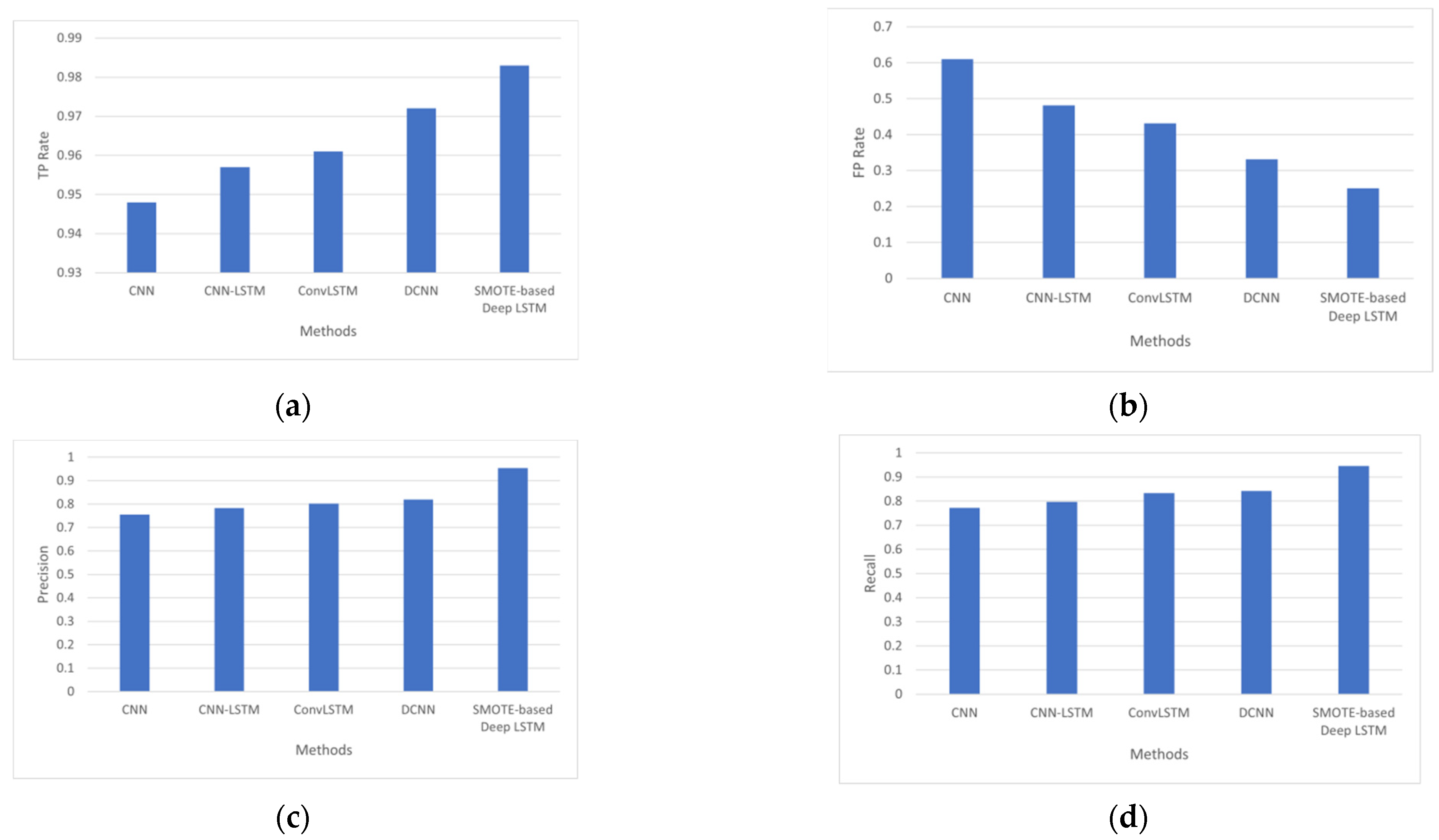
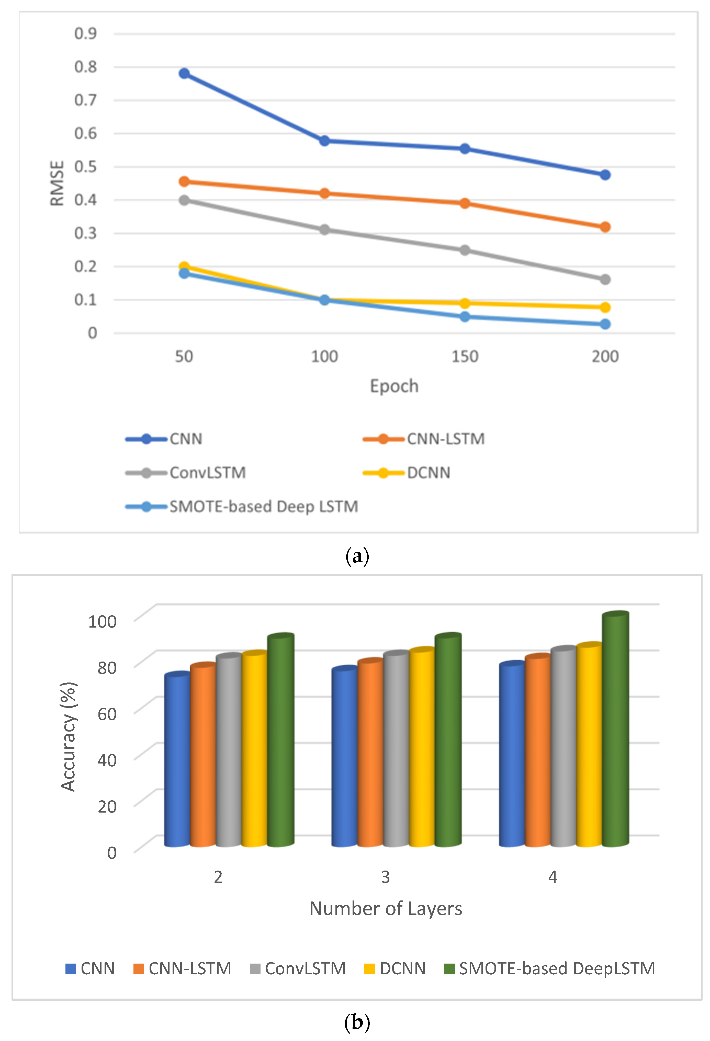
4.3. Results Analysis

The proposed model had two parts: class imbalance handling using the SMOTE followed by the deep LSTM classifier. The Pima Indian Diabetes Dataset was used to test proposed model. This research employed CNN, CNN-LSTM, ConvLSTM, and DCNN for measuring the classification performance. SMOTE was applied prior to these models and the performance was monitored. The performance metrics were precision, recall, accuracy, and AUC. The performance analysis of models such as CNN, CNN-LSTM, ConvLSTM, DCNN, and SMOTE-based deep LSTM is shown in

Table 5. Comparison of different deep-learning models.

Models	Precision	Recall	Accuracy	AUC
CNN	0.756	0.772	0.781	0.81
CNN-LSTM	0.783	0.797	0.813	0.836
ConvLSTM	0.802	0.833	0.846	0.858
DCNN	0.819	0.842	0.862	0.912
SMOTE-based Deep LSTM	0.954	0.946	0.996	0.983

. The SMOTE-based deep LSTM model showed good performance in diabetes prediction when compared to all the other models.

Figure 2 depicts the performance obtained by various diabetes-prediction methods, with the SMOTE-based deep LSTM model achieving the highest performance with a TP rate of 0.983, an FP rate of 0.251, precision of 0.954, and recall of 0.946. Using SMOTE-based deep LSTM and nine attributes from the PIDD, diabetes prediction was achieved with 99.64% accuracy.

The AUC is a measure of a classifier’s ability to distinguish between classes. Figure 3 shows the AUC of several models such as convolutional neural network (CNN), convolutional neural network-LSTM (CNN-LSTM), ConvLSTM, DCNN, and the proposed model, SMOTE-based deep LSTM. The AUC of the proposed method was 0.983 which is better than other deep-learning methods.

The confusion matrix explains the details of the number of instances correctly classified and number of instances incorrectly classified.

Table 6. Confusion matrix of CNN.

		Predicted Class
Actual Class		1	0
	1	430	68
	0	100	170

presents the confusion matrix of CNN and it shows that CNN correctly classified 422 instances as “class label 1” or “diabetic”, while 170 instances were correctly predicted as “class label 0” or “non-diabetic”.

Table 7. Confusion matrix of CNN-LSTM.

		Predicted Class
Actual Class		1	0
	1	445	43
	0	100	180

shows the confusion matrix of CNN-LSTM. It shows that 445 instances were true positive and 180 instances were true negative, with an accuracy of 81.3%.

Table 8. Confusion matrix of ConvLSTM.

		Predicted Class
Actual Class		1	0
	1	522	31
	0	87	128

shows the confusion matrix of ConvLSTM. It shows that a greater number of instances were correctly classified by ConvLSTM than by the CNN or CNN-LSTM networks.

Table 9. Confusion matrix of DCNN.

		Predicted Class
Actual Class		1	0
	1	582	25
	0	81	80

shows the confusion matrix of DCNN. It shows that 522 instances were correctly classified as “class label 1” and 80 instances were correctly classified as “class label 0” with an accuracy of 86.2%.

Table 10. Confusion matrix of SMOTE-based deep LSTM.

		Predicted Class
Actual Class		1	0
	1	665	2
	0	1	100

shows the confusion matrix of SMOTE-based deep LSTM. This shows that SMOTE-based deep LSTM is performed better than other models in classifying instances correctly by reducing false positives and false negatives.

Generally, the perfect likeliness value is of above 0.90 [40]. According to Figure 4, DCNN had a Kappa coefficient [43] of 0.89 and SMOTE-based deep LSTM had a Kappa coefficient of 0.94. Hence, SMOTE-based deep LSTM is a good classification model. The error term RMSE was found by comparing the outputs corresponding to each input. The RMSE of SMOTE-based deep LSTM was 0.051 less when compared to DCNN.

The mean absolute error (MAE) of benchmark models such as CNN, CNN-LSTM, ConvLSTM, DCNN, and the proposed model are presented in

Table 11. MAE of different deep-learning models.

Models	MAE
CNN	0.396
CNN-LSTM	0.239
ConvLSTM	0.082
DCNN	0.032
SMOTE-based Deep LSTM	0.013

. It shows that the MAE of SMOTE-based deep LSTM was less than that of other benchmark models.

The Figure 5a depicts the RMSE error for the epochs 50, 100, 150 and 200. The RMSE of proposed method is reduced to 0.027 when it reached 200 epoch. The Figure 5b shows accuracy of various deep-learning methods by varying the layers counted. These models were tested with two, three, and four layers. The proposed method with four layers achieved accuracy of 99.64% compared to other methods.

This is the best level of accuracy yet achieved in automated diabetes prediction using the PIDD. The advantages of our method are:

• The SMOTE-based deep LSTM model was introduced to diagnose type-2 diabetes using the PIDD as input.
• Class imbalance learning is also handled by SMOTE-based deep LSTM.
• The accuracy of automated diabetes prediction method is higher than that of other diabetes-prediction methods.

5. Conclusions

Using the Pima Indian Diabetes Dataset, the proposed technique predicted type-2 diabetes in females. Pregnancies, glucose, blood pressure, skin thickness, insulin, BMI, diabetes pedigree function, age, and outcome were all evaluated while doing multivariate time-series diabetes prediction. This paper applied deep-learning concepts to type-2 diabetic prediction modelling and attained the predicted results with the Pima Indian Diabetes Dataset. The SMOTE-based deep LSTM used in this paper quickly completed the characteristics of the whole process of class-imbalance handling and prediction. Using SMOTE-based deep LSTM, we can uncover hidden threats early and take preventive steps to improve the patient’s life and reduce diabetic risk. The proposed SMOTE-based deep LSTM performed well on the basis of accuracy and will be extended to predict other diseases from other medical data.

The limitations of the proposed methodology are as follows:

• The proposed method does not focus on treating intra-class imbalance;
• SMOTE-based Deep LSTM is not designed for the multiclass classification problem;
• The classification ability of the proposed method was evaluated only on the Pima Indian Diabetes Dataset.

The implications of our study for the research field are as follows:

• Inter-class imbalance commonly exists in binary-class datasets. The proposed method solves inter-class imbalance.
• In future, the proposed method can be extended to focus on intra-class imbalance. The proposed method performed binary classification on the Pima Indian Diabetes Dataset. It can be extended to work on multiclass datasets.
• SMOTE was used in this work as a data augmentation technique for class balancing. In the future, a generative adversarial network can be used for data augmentation.

References

1. Mishra, S.; Tripathy, H.K.; Mallick, P.K.; Bhoi, A.K.; Barsocchi, P. EAGA-MLP—An enhanced and adaptive hybrid classification model for diabetes diagnosis. Sensors 2020, 20, 4036. [Google Scholar] [CrossRef] [PubMed]
2. Swapna, G.; Vinayakumar, R.; Soman, K.P. Diabetes detection using deep learning algorithms. ICT Express 2018, 4, 243–246. [Google Scholar]
3. Sisodia, D.; Sisodia, D.S. Prediction of diabetes using classification algorithms. Procedia Comput. Sci. 2018, 132, 1578–1585. [Google Scholar] [CrossRef]
4. Learning, U.M. Pima Indians Diabetes Database. 2016. Available online: https://www.kaggle.com/datasets/uciml/pima-indians-diabetes-database (accessed on 5 May 2022).
5. Rakshit, S.; Manna, S.; Biswas, S.; Kundu, R.; Gupta, P.; Maitra, S.; Barman, S. Prediction of diabetes type-II using a two-class neural network. In Proceedings of the International Conference on Computational Intelligence, Communications, and Business Analytics, Kolkata, India, 24–25 March 2017; Springer: Singapore, 2017; pp. 65–71. [Google Scholar]
6. Alex, S.A.; Nayahi, J.; Shine, H.; Gopirekha, V. Deep convolutional neural network for diabetes mellitus prediction. Neural Comput. Appl. 2022, 34, 1319–1327. [Google Scholar] [CrossRef]
7. Chawla, N.V.; Bowyer, K.W.; Hall, L.O.; Kegelmeyer, W.P. SMOTE: Synthetic minority over-sampling technique. J. Artif. Intell. Res. 2002, 16, 321–357. [Google Scholar] [CrossRef]
8. Singh, A.; Ranjan, R.K.; Tiwari, A.; Naveena, S. Credit card fraud detection under extreme imbalanced data: A comparative study of data-level algorithms. J. Exp. Theor. Artif. Intell. 2022, 34, 571–598. [Google Scholar]
9. Han, W.; Huang, Z.; Li, S.; Jia, Y. Distribution-sensitive unbalanced data oversampling method for medical diagnosis. J. Med. Syst. 2019, 43, 39. [Google Scholar] [CrossRef]
10. Luukka, P.; Leppälampi, T. Similarity classifier with generalized mean applied to medical data. Comput. Biol. Med. 2006, 36, 1026–1040. [Google Scholar] [CrossRef]
11. Ahmad, F.; Mat Isa, N.A.; Hussain, Z.; Osman, M.K. Intelligent medical disease diagnosis using improved hybrid genetic algorithm-multilayer perceptron network. J. Med. Syst. 2013, 37, 9934. [Google Scholar] [CrossRef]
12. Christobel, Y.A.; Sivaprakasam, P. A new classwise k nearest neighbor (CKNN) method for the classification of diabetes dataset. Int. J. Eng. Adv. Technol. 2013, 2, 396–400. [Google Scholar]
13. Polat, K.; Güneş, S.; Arslan, A. A cascade learning system for classification of diabetes disease: Generalized discriminant analysis and least square support vector machine. Expert Syst. Appl. 2008, 34, 482–487. [Google Scholar] [CrossRef]
14. Abiodun,, O.I.; Jantan, A.; Omolara, A.E.; Dada, K.V.; Mohamed, N.A.; Arshad, H. State-of-the-art in artificial neural network applications: A survey. Heliyon 2018, 4, e00938. [Google Scholar]
15. Kahramanli, H.; Allahverdi, N. Design of a hybrid system for the diabetes and heart diseases. Expert Syst. Appl. 2008, 35, 82–89. [Google Scholar] [CrossRef]
16. Kayaer, K.; Yildirim, T. Medical diagnosis on Pima Indian diabetes using general regression neural networks. In Proceedings of the International Conference on Artificial Neural Networks and Neural Information Processing, Istanbul, Turkey, 26–29 June 2003; pp. 181–184. [Google Scholar]
17. Pokharel, M.; Alsadoon, A.; Nguyen, T.Q.V.; Al-Dala’in, T.; Pham, D.T.H.; Prasad, P.W.C.; Mai, H.T. Deep learning for predicting the onset of type 2 diabetes: Enhanced ensemble classifier using modified t-SNE. Multimed. Tools Appl. 2022, 81, 27837–27852. [Google Scholar] [CrossRef]
18. Vidhya, K.; Shanmugalakshmi, R. Deep learning based big medical data analytic model for diabetes complication prediction. J. Ambient. Intell. Humaniz. Comput. 2020, 11, 5691–5702. [Google Scholar] [CrossRef]
19. Mohebbi, A.; Aradottir, T.B.; Johansen, A.R.; Bengtsson, H.; Fraccaro, M.; Mørup, M. A deep learning approach to adherence detection for type 2 diabetics. In Proceedings of the 2017 39th Annual International Conference of the IEEE Engineering in Medicine and Biology Society, Jeju, Korea, 11–15 July 2017; pp. 2896–2899. [Google Scholar]
20. Caliskan, A.; Yuksel, M.E.; Badem, H.; Basturk, A. Performance improvement of deep neural network classifiers by a simple training strategy. Eng. Appl. Artif. Intell. 2018, 67, 14–23. [Google Scholar] [CrossRef]
21. Pham, T.; Tran, T.; Phung, D.; Venkatesh, S. Predicting healthcare trajectories from medical records: A deep learning approach. J. Biomed. Inform. 2017, 69, 218–229. [Google Scholar] [CrossRef]
22. Sun, J.; Li, H.; Fujita, H.; Fu, B.; Ai, W. Class-imbalanced dynamic financial distress prediction based on Adaboost-SVM ensemble combined with SMOTE and time weighting. Inf. Fusion 2020, 54, 128–144. [Google Scholar] [CrossRef]
23. Temurtas, H.; Yumusak, N.; Temurtas, F. A comparative study on diabetes disease diagnosis using neural networks. Expert Syst. Appl. 2009, 36, 8610–8615. [Google Scholar] [CrossRef]
24. Dwivedi, A.K. Analysis of computational intelligence techniques for diabetes mellitus prediction. Neural Comput. Appl. 2018, 30, 3837–3845. [Google Scholar] [CrossRef]
25. Swapna, G.; Kp, S.; Vinayakumar, R. Automated detection of diabetes using CNN and CNN-LSTM network and heart rate signals. Procedia Comput. Sci. 2018, 132, 1253–1262. [Google Scholar]
26. Rabby, M.F.; Tu, Y.; Hossen, M.I.; Lee, I.; Maida, A.S.; Hei, X. Stacked LSTM based deep recurrent neural network with kalman smoothing for blood glucose prediction. BMC Med. Inform. Decis. Mak. 2021, 21, 101. [Google Scholar] [CrossRef] [PubMed]
27. Kutlu, H.; Avcı, E. A novel method for classifying liver and brain tumors using convolutional neural networks, discrete wavelet transform and long short-term memory networks. Sensors 2019, 19, 1992. [Google Scholar] [CrossRef] [PubMed]
28. Rahman, M.; Islam, D.; Mukti, R.J.; Saha, I. A deep learning approach based on convolutional LSTM for detecting diabetes. Comput. Biol. Chem. 2020, 88, 107329. [Google Scholar] [CrossRef] [PubMed]
29. Hochreiter, S. Ja1 4 rgen schmidhuber. Long short-term memory. Neural Comput. 1997, 9, 1735–1780. [Google Scholar] [CrossRef]
30. Chang, V.; Bailey, J.; Xu, Q.A.; Sun, Z. Pima Indians diabetes mellitus classification based on machine learning (ML) algorithms. Neural Comput. Appl. 2022, 1–17. [Google Scholar] [CrossRef]
31. Chang, P.; Grinband, J.; Weinberg, B.D.; Bardis, M.; Khy, M.; Cadena, G.; Chow, D. Deep-learning convolutional neural networks accurately classify genetic mutations in gliomas. Am. J. Neuroradiol. 2018, 39, 1201–1207. [Google Scholar] [CrossRef]
32. Dorffner, G. Neural networks for time series processing. In Proceedings of the Neural Network World; 1996. Available online: https://citeseerx.ist.psu.edu/viewdoc/download;jsessionid=02C8586DF982ABE36E5775BF3E86642E?doi=10.1.1.45.5697&rep=rep1&type=pdf (accessed on 10 January 2022).
33. Kingma, D.P.; Ba, J. Adam: A method for stochastic optimization. arXiv 2014, arXiv:1412.6980. [Google Scholar]
34. Zhao, H.; Hou, C.; Alrobassy, H.; Zeng, X. Recognition of transportation state by smartphone sensors using deep bi-LSTM neural network. J. Comput. Netw. Commun. 2019, 2019, 4967261. [Google Scholar] [CrossRef]
35. Sunny, M.A.I.; Maswood, M.M.S.; Alharbi, A.G. Deep learning-based stock price prediction using LSTM and bi-directional LSTM model. In Proceedings of the 2020 2nd Novel Intelligent and Leading Emerging Sciences Conference (NILES), Giza, Egypt, 24–26 October 2020; IEEE: Piscataway, NJ, USA, 2020; pp. 87–92. [Google Scholar]
36. Sun, B.; Liu, M.; Zheng, R.; Zhang, S. Attention-based LSTM network for wearable human activity recognition. In Proceedings of the 2019 Chinese Control Conference (CCC), Guangzhou, China, 27–30 July 2019; IEEE: Piscataway, NJ, USA, 2019; pp. 8677–8682. [Google Scholar]
37. Rajagukguk, R.A.; Kamil, R.; Lee, H.J. A Deep Learning Model to Forecast Solar Irradiance Using a Sky Camera. Appl. Sci. 2021, 11, 5049. [Google Scholar] [CrossRef]
38. Zhu, Z.; Wang, H.; Liu, Z.; Meng, S. Fault diagnosis of wheelset bearings using deep bidirectional long short-term memory network. In Proceedings of the 2019 Prognostics and System Health Management Conference (PHM-Qingdao), Qingdao, China, 25–27 October 2019; pp. 1–7. [Google Scholar]
39. Zhang, T.; Song, S.; Li, S.; Ma, L.; Pan, S.; Han, L. Research on gas concentration prediction models based on LSTM multidimensional time series. Energies 2019, 12, 161. [Google Scholar] [CrossRef]
40. Du, Y.; Wang, W.; Wang, L. Hierarchical recurrent neural network for skeleton based action recognition. In Proceedings of the IEEE Conference on Computer Vision and Pattern Recognition, Boston, MA, USA, 7 June 2015; IEEE: Piscataway, NJ, USA, 2015; pp. 1110–1118. [Google Scholar]
41. Majhi, B.; Naidu, D.; Mishra, A.P.; Satapathy, S.C. Improved prediction of daily pan evaporation using Deep-LSTM model. Neural Comput. Appl. 2020, 32, 7823–7838. [Google Scholar] [CrossRef]
42. Phan, H.; Andreotti, F.; Cooray, N.; Chén, O.Y.; De Vos, M. DNN filter bank improves 1-max pooling CNN for single-channel EEG automatic sleep stage classification. In Proceedings of the 2018 40th Annual International Conference of the IEEE Engineering in Medicine and Biology Society (EMBC), Honolulu, HI, USA, 18–21 July 2018; IEEE: Piscataway, NJ, USA, 2018; pp. 453–456. [Google Scholar]
43. McHugh, M.L. Interrater reliability: The kappa statistic. Biochem. Med. 2012, 22, 276–282. [Google Scholar] [CrossRef]
Figure 1. SMOTE-based deep LSTM for diabetic prediction.
Electronics 11 02737 g001
Figure 2. (a) Analysis based on TP Rate, (b) analysis based on FP Rate, (c) analysis based on precision, and (d) analysis based on recall.
Electronics 11 02737 g002
Figure 3. AUC of SMOTE-based deep LSTM.
Electronics 11 02737 g003
Figure 4. Errors of different deep-learning models.
Electronics 11 02737 g004
Figure 5. Performance of SMOTE-based deep LSTM. (a) Epoch vs. loss and (b) layers vs. accuracy.
Electronics 11 02737 g005