
CSGN: Combined Channel- and Spatial-Wise Dynamic Gating Architecture for Convolutional Neural Networks


Abstract
:1. Introduction
- 1.
- We propose a fine-grained gating architecture combining channel- and spatial-wise sparsity to design computation-efficient architecture on the fly.
- 2.
- Two gating modules, CG and SG, can be integrated into the CNNs and utilized with the existing gradient-based optimizers. Additionally, we encourage two gating modules by introducing sparse training loss to enable end-to-end training.
- 3.
- The performance of CSGN onthe widely used image classification datasets CIFAR-10 and ImageNet, and the object detection dataset MS COCO is validated to demonstrate the combined effect. Furthermore, compared to other dynamic gating networks and static methods, the proposed network achieves competitive results.
2. Related Work
2.1. Layer-Wise Gating Architecture
2.2. Channel-Wise Gating Architecture
2.3. Spatial-Wise Gating Architecture
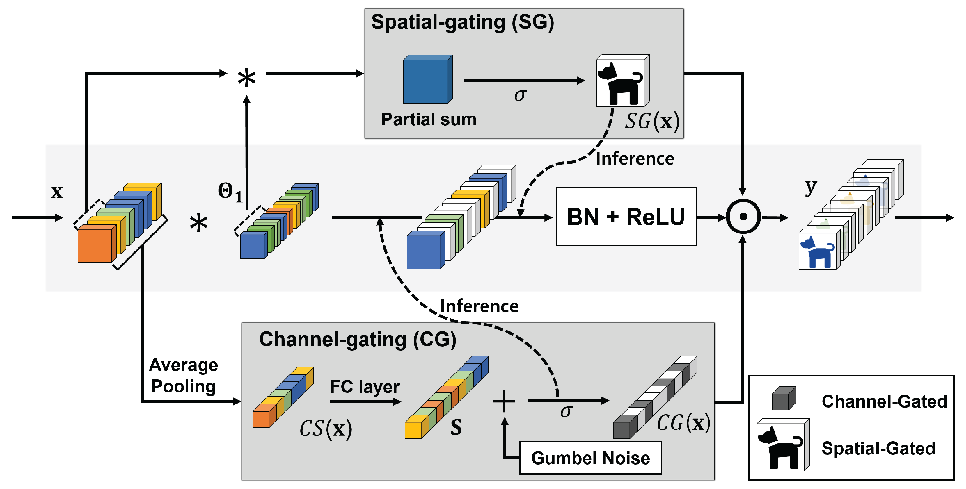
3. CSGN
3.1. Gating Architecture
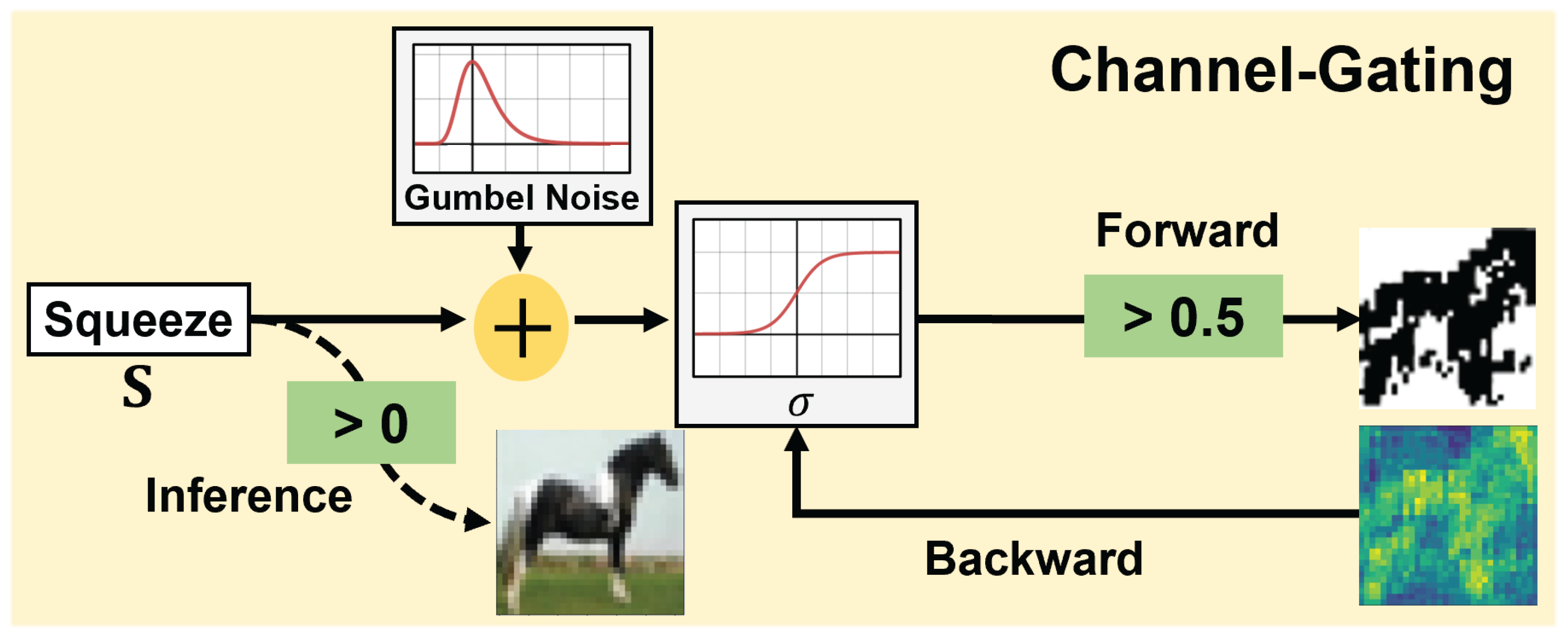
3.2. CG Module
3.2.1. Channel Squeezing
3.2.2. Binary Gumbel-Softmax Trick
3.3. SG Module
3.4. Inference on CSGN
3.5. Sparsity Training Loss
4. Evaluation
4.1. Experimental Setup
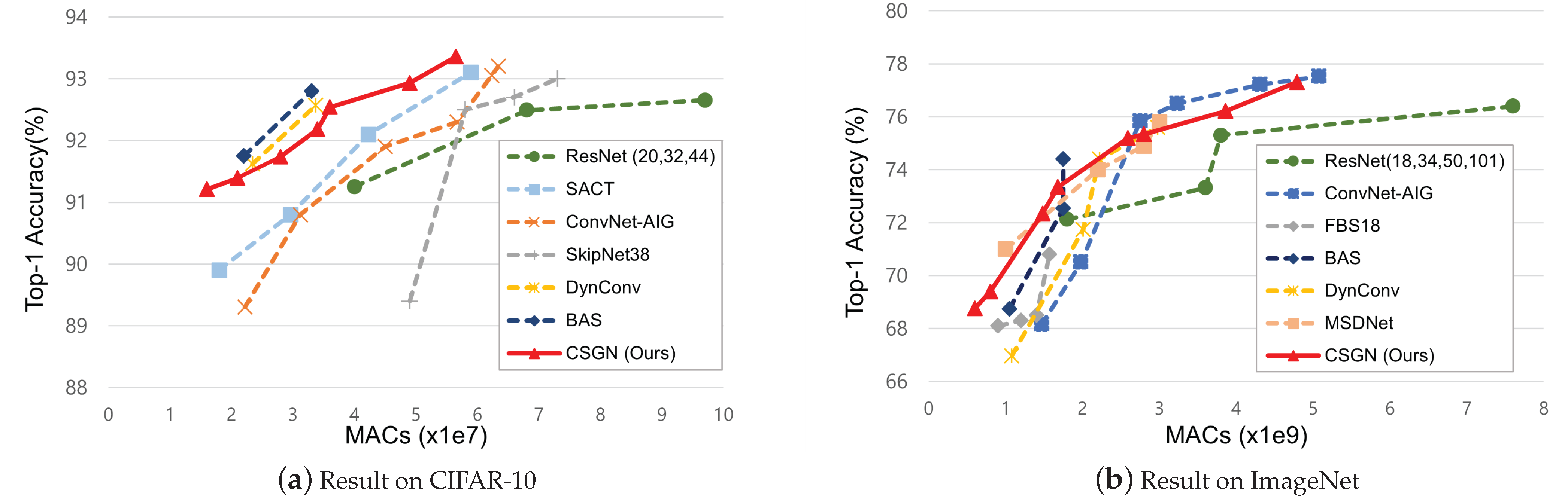
4.2. CIFAR-10
4.3. Imagenet
4.4. Ms Coco
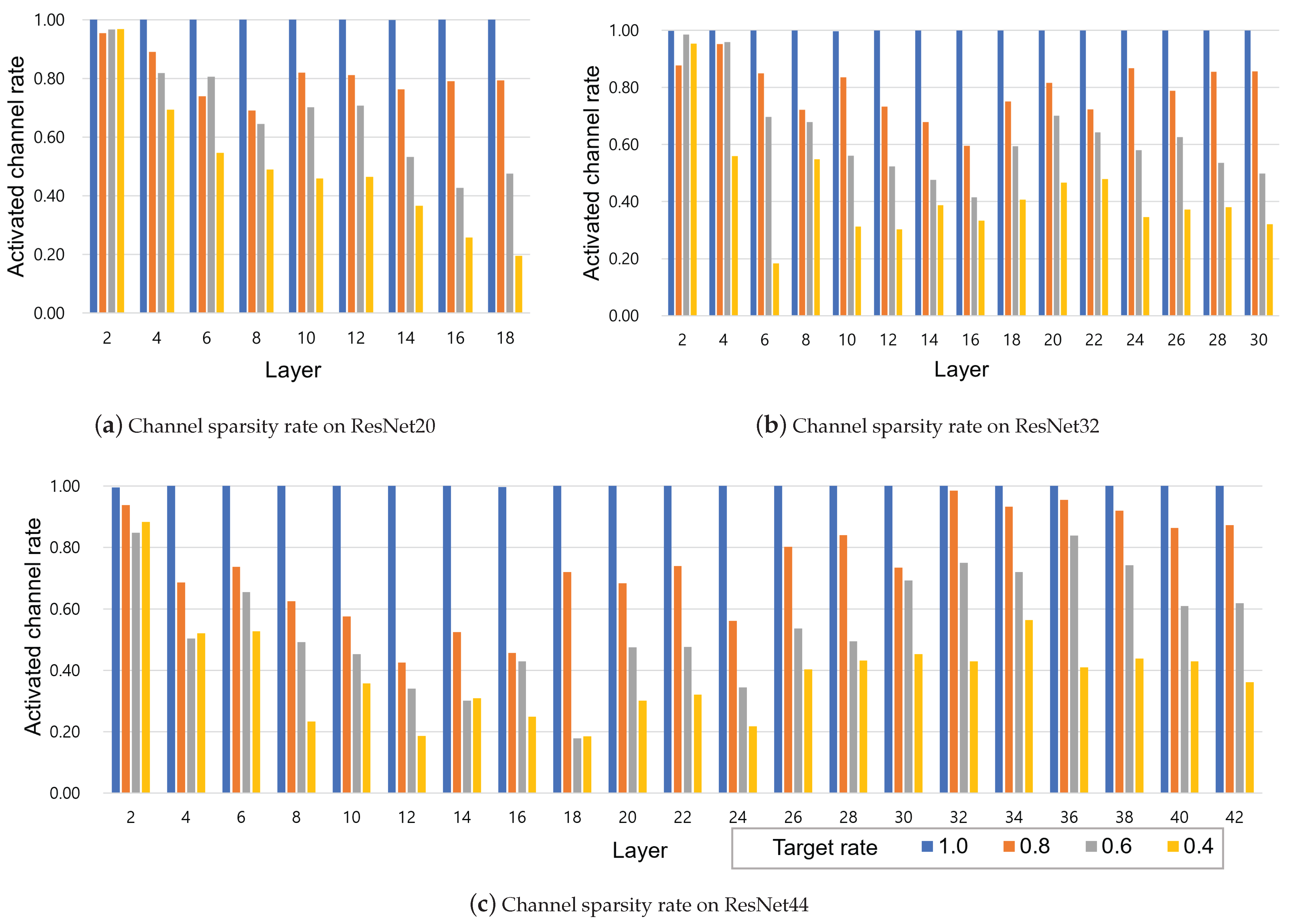
4.5. Ablation Study
4.6. Additional Analysis
5. Conclusions
Author Contributions
Funding
Conflicts of Interest
References
- Alom, M.Z.; Taha, T.M.; Yakopcic, C.; Westberg, S.; Sidike, P.; Nasrin, M.S.; Hasan, M.; Van Essen, B.C.; Awwal, A.A.; Asari, V.K. A state-of-the-art survey on deep learning theory and architectures. Electronics 2019, 8, 292. [Google Scholar] [CrossRef]
- Zeng, X.; Wang, Z.; Hu, Y. Enabling Efficient Deep Convolutional Neural Network-based Sensor Fusion for Autonomous Driving. arXiv 2022, arXiv:2202.11231. [Google Scholar]
- Cuong-Le, T.; Nghia-Nguyen, T.; Khatir, S.; Trong-Nguyen, P.; Mirjalili, S.; Nguyen, K.D. An efficient approach for damage identification based on improved machine learning using PSO-SVM. Eng. Comput. 2021, 38, 3069–3084. [Google Scholar] [CrossRef]
- Maor, G.; Zeng, X.; Wang, Z.; Hu, Y. An FPGA implementation of stochastic computing-based LSTM. In Proceedings of the 2019 IEEE 37th International Conference on Computer Design (ICCD), Abu Dhabi, United Arab Emirates, 17–20 November 2019; IEEE: Abu Dhabi, United Arab Emirates, 2019; pp. 38–46. [Google Scholar]
- Chen, J.; Ran, X. Deep learning with edge computing: A review. Proc. IEEE 2019, 107, 1655–1674. [Google Scholar] [CrossRef]
- Canziani, A.; Paszke, A.; Culurciello, E. An analysis of deep neural network models for practical applications. arXiv 2016, arXiv:1605.07678. [Google Scholar]
- Liang, T.; Glossner, J.; Wang, L.; Shi, S.; Zhang, X. Pruning and quantization for deep neural network acceleration: A survey. Neurocomputing 2021, 461, 370–403. [Google Scholar] [CrossRef]
- Kim, Y.D.; Park, E.; Yoo, S.; Choi, T.; Yang, L.; Shin, D. Compression of deep convolutional neural networks for fast and low power mobile applications. arXiv 2015, arXiv:1511.06530. [Google Scholar]
- Han, S.; Mao, H.; Dally, W.J. Deep compression: Compressing deep neural networks with pruning, trained quantization and huffman coding. arXiv 2015, arXiv:1510.00149. [Google Scholar]
- Bengio, Y. Deep learning of representations: Looking forward. In Proceedings of the International Conference on Statistical Language and Speech Processing, Tarragona, Spain, 29–31 July 2013; Springer: Berlin/Heidelberg, Germany, 2013; pp. 1–37. [Google Scholar]
- Sigaud, O.; Masson, C.; Filliat, D.; Stulp, F. Gated networks: An inventory. arXiv 2015, arXiv:1512.03201. [Google Scholar]
- Zhou, X.; Zhang, W.; Xu, H.; Zhang, T. Effective sparsification of neural networks with global sparsity constraint. In Proceedings of the IEEE/CVF Conference on Computer Vision and Pattern Recognition, Nashville, TN, USA, 19–25 June 2021; pp. 3599–3608. [Google Scholar]
- He, Y.; Kang, G.; Dong, X.; Fu, Y.; Yang, Y. Soft filter pruning for accelerating deep convolutional neural networks. arXiv 2018, arXiv:1808.06866. [Google Scholar]
- He, Y.; Liu, P.; Wang, Z.; Hu, Z.; Yang, Y. Filter pruning via geometric median for deep convolutional neural networks acceleration. In Proceedings of the IEEE/CVF Conference on Computer Vision and Pattern Recognition, Long Beach, CA, USA, 15–20 June 2019; pp. 4340–4349. [Google Scholar]
- Liu, Z.; Li, J.; Shen, Z.; Huang, G.; Yan, S.; Zhang, C. Learning efficient convolutional networks through network slimming. In Proceedings of the IEEE International Conference on Computer Vision, Venice, Italy, 22–29 October 2017; pp. 2736–2744. [Google Scholar]
- Howard, A.G.; Zhu, M.; Chen, B.; Kalenichenko, D.; Wang, W.; Weyand, T.; Andreetto, M.; Adam, H. Mobilenets: Efficient convolutional neural networks for mobile vision applications. arXiv 2017, arXiv:1704.04861. [Google Scholar]
- Zhang, X.; Zhou, X.; Lin, M.; Sun, J. Shufflenet: An extremely efficient convolutional neural network for mobile devices. In Proceedings of the IEEE Conference on Computer Vision and Pattern Recognition, Salt Lake City, UT, USA, 18–22 June 2018; pp. 6848–6856. [Google Scholar]
- Sandler, M.; Howard, A.; Zhu, M.; Zhmoginov, A.; Chen, L.C. Mobilenetv2: Inverted residuals and linear bottlenecks. In Proceedings of the IEEE Conference on Computer Vision and Pattern Recognition, Salt Lake City, UT, USA, 18–22 June 2018; pp. 4510–4520. [Google Scholar]
- Tan, M.; Chen, B.; Pang, R.; Vasudevan, V.; Sandler, M.; Howard, A.; Le, Q.V. Mnasnet: Platform-aware neural architecture search for mobile. In Proceedings of the IEEE/CVF Conference on Computer Vision and Pattern Recognition, Long Beach, CA, USA, 15–20 June 2019; pp. 2820–2828. [Google Scholar]
- Hinton, G.; Vinyals, O.; Dean, J. Distilling the knowledge in a neural network. arXiv 2015, arXiv:1503.02531. [Google Scholar]
- Ba, J.; Caruana, R. Do deep nets really need to be deep? In Proceedings of the Advances in Neural Information Processing Systems, Montreal, QC, Canada, 8–13 December 2014; pp. 2654–2662. [Google Scholar]
- Romero, A.; Ballas, N.; Kahou, S.E.; Chassang, A.; Gatta, C.; Bengio, Y. Fitnets: Hints for thin deep nets. arXiv 2014, arXiv:1412.6550. [Google Scholar]
- Zagoruyko, S.; Komodakis, N. Paying more attention to attention: Improving the performance of convolutional neural networks via attention transfer. arXiv 2016, arXiv:1612.03928. [Google Scholar]
- Yim, J.; Joo, D.; Bae, J.; Kim, J. A gift from knowledge distillation: Fast optimization, network minimization and transfer learning. In Proceedings of the IEEE Conference on Computer Vision and Pattern Recognition, Honolulu, HI, USA, 21–26 July 2017; pp. 4133–4141. [Google Scholar]
- Zhou, S.; Wu, Y.; Ni, Z.; Zhou, X.; Wen, H.; Zou, Y. Dorefa-net: Training low bitwidth convolutional neural networks with low bitwidth gradients. arXiv 2016, arXiv:1606.06160. [Google Scholar]
- Lin, X.; Zhao, C.; Pan, W. Towards accurate binary convolutional neural network. In Proceedings of the Advances in Neural Information Processing Systems, Long Beach, CA, USA, 4–9 December 2017. [Google Scholar]
- Rastegari, M.; Ordonez, V.; Redmon, J.; Farhadi, A. Xnor-net: Imagenet classification using binary convolutional neural networks. In Proceedings of the European Conference on Computer Vision, Amsterdam, The Netherlands, 8–16 October 2016; Springer: Berlin/Heidelberg, Germany, 2016; pp. 525–542. [Google Scholar]
- Hubara, I.; Courbariaux, M.; Soudry, D.; El-Yaniv, R.; Bengio, Y. Binarized neural networks. In Proceedings of the 30th International Conference on Neural Information Processing Systems, Barcelona, Spain, 5–10 December 2016; pp. 4114–4122. [Google Scholar]
- Li, S.; Hanson, E.; Li, H.; Chen, Y. Penni: Pruned kernel sharing for efficient CNN inference. In Proceedings of the International Conference on Machine Learning, Virtual Event, 13–18 July 2020; pp. 5863–5873. [Google Scholar]
- Li, S.; Hanson, E.; Qian, X.; Li, H.H.; Chen, Y. ESCALATE: Boosting the Efficiency of Sparse CNN Accelerator with Kernel Decomposition. In Proceedings of the MICRO-54: 54th Annual IEEE/ACM International Symposium on Microarchitecture, Virtual Event, 18–22 October 2021; pp. 992–1004. [Google Scholar]
- Denton, E.L.; Zaremba, W.; Bruna, J.; LeCun, Y.; Fergus, R. Exploiting linear structure within convolutional networks for efficient evaluation. Adv. Neural Inf. Process. Syst. 2014, 1, 1269–1277. [Google Scholar]
- Graves, A. Adaptive computation time for recurrent neural networks. arXiv 2016, arXiv:1603.08983. [Google Scholar]
- Bolukbasi, T.; Wang, J.; Dekel, O.; Saligrama, V. Adaptive neural networks for efficient inference. In Proceedings of the International Conference on Machine Learning. PMLR, Sydney, Australia, 6–11 August 2017; pp. 527–536. [Google Scholar]
- Panda, P.; Sengupta, A.; Roy, K. Conditional deep learning for energy-efficient and enhanced pattern recognition. In Proceedings of the 2016 Design, Automation & Test in Europe Conference & Exhibition (DATE), Dresden, Germany, 14–18 March 2016; IEEE: Dresden, Germany, 2016; pp. 475–480. [Google Scholar]
- Huang, G.; Chen, D.; Li, T.; Wu, F.; Van Der Maaten, L.; Weinberger, K.Q. Multi-scale dense networks for resource efficient image classification. arXiv 2017, arXiv:1703.09844. [Google Scholar]
- Veit, A.; Belongie, S. Convolutional networks with adaptive inference graphs. In Proceedings of the European Conference on Computer Vision (ECCV), Munich, Germany, 8–14 September 2018; pp. 3–18. [Google Scholar]
- Wang, X.; Yu, F.; Dou, Z.Y.; Darrell, T.; Gonzalez, J.E. Skipnet: Learning dynamic routing in convolutional networks. In Proceedings of the European Conference on Computer Vision (ECCV), Munich, Germany, 8–14 September 2018; pp. 409–424. [Google Scholar]
- Wu, Z.; Nagarajan, T.; Kumar, A.; Rennie, S.; Davis, L.S.; Grauman, K.; Feris, R. Blockdrop: Dynamic inference paths in residual networks. In Proceedings of the IEEE Conference on Computer Vision and Pattern Recognition, Salt Lake City, UT, USA, 18–22 June 2018; pp. 8817–8826. [Google Scholar]
- Chen, Z.; Li, Y.; Bengio, S.; Si, S. You look twice: Gaternet for dynamic filter selection in cnns. In Proceedings of the IEEE/CVF Conference on Computer Vision and Pattern Recognition, Long Beach, CA, USA, 15–20 June 2019; pp. 9172–9180. [Google Scholar]
- Gao, X.; Zhao, Y.; Dudziak, Ł.; Mullins, R.; Xu, C.Z. Dynamic channel pruning: Feature boosting and suppression. arXiv 2018, arXiv:1810.05331. [Google Scholar]
- Bejnordi, B.E.; Blankevoort, T.; Welling, M. Batch-shaping for learning conditional channel gated networks. arXiv 2019, arXiv:1907.06627. [Google Scholar]
- Hua, W.; Zhou, Y.; De Sa, C.M.; Zhang, Z.; Suh, G.E. Channel gating neural networks. Adv. Neural Inf. Process. Syst. 2019, 32, 1886–1896. [Google Scholar]
- Zhou, B.; Khosla, A.; Lapedriza, A.; Oliva, A.; Torralba, A. Learning deep features for discriminative localization. In Proceedings of the IEEE Conference on Computer Vision and Pattern Recognition, Las Vegas, NV, USA, 27–30 June 2016; pp. 2921–2929. [Google Scholar]
- Figurnov, M.; Collins, M.D.; Zhu, Y.; Zhang, L.; Huang, J.; Vetrov, D.; Salakhutdinov, R. Spatially adaptive computation time for residual networks. In Proceedings of the IEEE Conference on Computer Vision and Pattern Recognition, Honolulu, HI, USA, 21–26 July 2017; pp. 1039–1048. [Google Scholar]
- Verelst, T.; Tuytelaars, T. Dynamic convolutions: Exploiting spatial sparsity for faster inference. In Proceedings of the IEEE/CVF Conference on Computer Vision and Pattern Recognition, Seattle, WA, USA, 14–19 June 2020; pp. 2320–2329. [Google Scholar]
- Wang, Y.; Lv, K.; Huang, R.; Song, S.; Yang, L.; Huang, G. Glance and focus: A dynamic approach to reducing spatial redundancy in image classification. Adv. Neural Inf. Process. Syst. 2020, 33, 2432–2444. [Google Scholar]
- Lin, J.; Rao, Y.; Lu, J.; Zhou, J. Runtime neural pruning. Adv. Neural Inf. Process. Syst. 2017, 30, 2178–2188. [Google Scholar]
- Cao, S.; Ma, L.; Xiao, W.; Zhang, C.; Liu, Y.; Zhang, L.; Nie, L.; Yang, Z. Seernet: Predicting convolutional neural network feature-map sparsity through low-bit quantization. In Proceedings of the IEEE/CVF Conference on Computer Vision and Pattern Recognition, Long Beach, CA, USA, 16–19 June 2019; pp. 11216–11225. [Google Scholar]
- He, K.; Zhang, X.; Ren, S.; Sun, J. Deep residual learning for image recognition. In Proceedings of the IEEE Conference on Computer Vision and Pattern Recognition, Las Vegas, NV, USA, 1–26 June 2016; pp. 770–778. [Google Scholar]
- Jang, E.; Gu, S.; Poole, B. Categorical reparameterization with gumbel-softmax. arXiv 2016, arXiv:1611.01144. [Google Scholar]
- Krizhevsky, A.; Hinton, G. Learning Multiple Layers of Features from Tiny Images. Master’s Thesis, Department of Computer Science, University of Toronto, Toronto, ON, Canada, 2009. [Google Scholar]
- Deng, J.; Dong, W.; Socher, R.; Li, L.J.; Li, K.; Fei-Fei, L. Imagenet: A large-scale hierarchical image database. In Proceedings of the 2009 IEEE Conference on Computer Vision and Pattern Recognition, Miami, FL, USA, 20–25 June 2009; IEEE: Miami, FL, USA, 2009; pp. 248–255. [Google Scholar]
- He, K.; Zhang, X.; Ren, S.; Sun, J. Delving deep into rectifiers: Surpassing human-level performance on imagenet classification. In Proceedings of the IEEE International Conference on Computer Vision, Washington, DC, USA, 7–13 December 2015; pp. 1026–1034. [Google Scholar]
- Lin, T.Y.; Goyal, P.; Girshick, R.; He, K.; Dollár, P. Focal loss for dense object detection. In Proceedings of the IEEE International Conference on Computer Vision, Venice, Italy, 22–29 October 2017; pp. 2980–2988. [Google Scholar]
- Lin, T.Y.; Dollár, P.; Girshick, R.; He, K.; Hariharan, B.; Belongie, S. Feature pyramid networks for object detection. In Proceedings of the IEEE Conference on Computer Vision and Pattern Recognition, Honolulu, HI, USA, 21–26 July 2017; pp. 2117–2125. [Google Scholar]
- Lin, T.Y.; Maire, M.; Belongie, S.; Hays, J.; Perona, P.; Ramanan, D.; Dollár, P.; Zitnick, C.L. Microsoft coco: Common objects in context. In Proceedings of the European Conference on Computer Vision, Zurich, Switzerland, 6–12 September 2014; Springer: Berlin/Heidelberg, Germany, 2014; pp. 740–755. [Google Scholar]


| Static Pruning | ProbMask [12], Soft Filter Pruning [13], FPGM [14], Network Slimming [15] | ||
|---|---|---|---|
| Dynamic gating architecture | Layer-wise | Early-exit | ACT [32], Bolukbasi et al. [33], Panda et al. [34], MSDNet [35] |
| Layer-skipping | ConvNet-AIG [36], SkipNet [37], Blockdrop [38] | ||
| Channel-wise | GaterNet [39], FBS [40], BAS [41], CGNet [42] | ||
| Spatial-wise | Zhou et al. [43], SACT [44], DynConv [45], GFNet [46] | ||
| Notations | Descriptions |
|---|---|
| Weight of the lth convolutional layer | |
| x, y | Input and output feature map |
| Height, width, channels, and filters at the lth layer | |
| Sigmoid function | |
| * | Naïve convolution operation |
| g | Identical and independent distribution samples from Gumbel distribution |
| Categorical distribution with class probabilities | |
| Temperature for Gumbel-SoftMax | |
| Sparsity loss function for CG and SG | |
| Threshold parameter of SG | |
| Target rate in CG and threshold target in SG | |
| Convolutional layers 1 and 2 in the residual block | |
| Average pooling function | |
| Saliency of channels | |
| CG output mask | |
| SG output mask |
| Baseline | 0.0 | 0.5 | |||||||
|---|---|---|---|---|---|---|---|---|---|
| 1.0 | 0.8 | 0.6 | 0.4 | 1.0 | 0.8 | 0.6 | 0.4 | ||
| ResNet20 | Accuracy (%) | 91.39 | 91.21 | 90.18 | 88.68 | 90.18 | 89.26 | 87.78 | 86.47 |
| MAC reduction | 1.97× | 2.46× | 2.81× | 3.82× | 3.62× | 4.53× | 5.31× | 7.11× | |
| ResNet32 | Accuracy (%) | 92.18 | 91.74 | 91.76 | 90.58 | 90.99 | 90.79 | 89.03 | 88.27 |
| MAC reduction | 1.99× | 2.47× | 3.11× | 4.64× | 3.89× | 4.48× | 5.58× | 7.98× | |
| ResNet44 | Accuracy (%) | 92.93 | 92.54 | 91.84 | 90.55 | 91.67 | 90.71 | 89.68 | 89.24 |
| MAC reduction | 1.98× | 2.71× | 3.73× | 5.09× | 4.01× | 5.39× | 6.83× | 9.51× | |
| ResNet110 | Accuracy (%) | 93.36 | 92.88 | 91.91 | 90.74 | 88.98 | 86.21 | 84.65 | 82.43 |
| MAC reduction | 2.10× | 3.05× | 4.48× | 5.49× | 6.13× | 9.18× | 10.42× | 11.78× | |
| Baseline | 0.0 | 0.5 | |||||||
|---|---|---|---|---|---|---|---|---|---|
| 1.0 | 0.8 | 0.6 | 0.4 | 1.0 | 0.8 | 0.6 | 0.4 | ||
| ResNet18 | Accuracy (%) | 70.21 | 69.39 | 65.22 | 63.03 | 69.12 | 68.76 | 64.14 | 63.08 |
| MAC reduction | 2.18× | 4.12× | 6.78× | 8.12× | 3.81× | 5.37× | 8.20× | 13.12× | |
| ResNet34 | Accuracy (%) | 74.42 | 73.35 | 69.54 | 68.24 | 72.85 | 72.35 | 69.19 | 67.31 |
| MAC reduction | 2.16× | 2.46× | 4.08× | 7.34× | 3.69× | 4.33× | 5.91× | 9.16× | |
| ResNet50 | Accuracy (%) | 75.34 | 75.19 | 74.14 | 72.73 | 75.08 | 73.86 | 71.70 | 69.60 |
| MAC reduction | 1.37× | 1.49× | 1.61× | 1.74× | 1.43× | 1.57× | 1.72× | 1.88× | |
| ResNet101 | Accuracy (%) | 77.31 | 76.21 | 74.92 | 74.02 | 75.83 | 74.21 | 72.01 | 70.24 |
| MAC reduction | 1.38× | 1.47× | 1.58× | 1.71× | 1.80× | 1.87× | 2.09× | 2.14× | |
| Model | AP | MAC Reduction | |||
|---|---|---|---|---|---|
| RetinaNet [54] | Baseline | 33.9 | 53.1 | 36.3 | 1.00× |
| CSGN (0.8/0.0) | 33.5 | 52.6 | 35.8 | 1.48× | |
| CSGN (0.6/0.0) | 33.3 | 52.4 | 35.7 | 1.63× | |
| Faster-RCNN [55] | Baseline | 34.3 | 55.9 | 37.7 | 1.00× |
| CSGN (0.8/0.0) | 33.9 | 55.6 | 37.3 | 1.47× | |
| CSGN (0.6/0.0) | 33.8 | 55.4 | 37.1 | 1.61× | |
| Accuracy (%) | Sparsity (%) | MAC () | |
|---|---|---|---|
| 0.8 | 92.43 | 21.60 | 3.43 |
| 0.7 | 92.20 | 31.40 | 3.12 |
| 0.6 | 91.85 | 40.70 | 2.77 |
| 0.5 | 90.92 | 50.50 | 2.32 |
| 0.4 | 91.05 | 60.10 | 1.85 |
| 0.3 | 90.08 | 70.03 | 1.45 |
| Accuracy (%) | Sparsity (%) | MAC () | ||
|---|---|---|---|---|
| 1.0 | 0.0 | 91.37 | 49.90 | 2.07 |
| 0.5 | 91.35 | 73.10 | 1.73 | |
| 1.0 | 90.63 | 72.30 | 1.56 | |
| 1.5 | 90.39 | 95.50 | 1.29 | |
| 2.0 | 90.05 | 99.40 | 0.91 | |
| 2.0 | 0.0 | 91.39 | 49.80 | 2.06 |
| 0.5 | 90.18 | 74.50 | 1.69 | |
| 1.0 | 90.08 | 89.10 | 1.46 | |
| 1.5 | 89.96 | 96.10 | 1.17 | |
| 2.0 | 89.96 | 96.10 | 0.87 |
| 1/p | Accuracy Drop (%) | |
|---|---|---|
| 2.0 | 2 | 0.37 |
| 4 | 0.56 | |
| 8 | 1.18 | |
| 16 | 1.48 | |
| 1.0 | 2 | 0.51 |
| 4 | 0.97 | |
| 8 | 1.23 | |
| 16 | 1.60 |
Publisher’s Note: MDPI stays neutral with regard to jurisdictional claims in published maps and institutional affiliations. |
© 2022 by the authors. Licensee MDPI, Basel, Switzerland. This article is an open access article distributed under the terms and conditions of the Creative Commons Attribution (CC BY) license (https://creativecommons.org/licenses/by/4.0/).
Share and Cite
Hyun, S.; Ryu, C.H.; Kang, J.Y.; Lim, H.J.; Han, T.H. CSGN: Combined Channel- and Spatial-Wise Dynamic Gating Architecture for Convolutional Neural Networks. Electronics 2022, 11, 2678. https://doi.org/10.3390/electronics11172678
Hyun S, Ryu CH, Kang JY, Lim HJ, Han TH. CSGN: Combined Channel- and Spatial-Wise Dynamic Gating Architecture for Convolutional Neural Networks. Electronics. 2022; 11(17):2678. https://doi.org/10.3390/electronics11172678
Chicago/Turabian StyleHyun, Sangmin, Chang Ho Ryu, Ju Yeon Kang, Hyun Jo Lim, and Tae Hee Han. 2022. "CSGN: Combined Channel- and Spatial-Wise Dynamic Gating Architecture for Convolutional Neural Networks" Electronics 11, no. 17: 2678. https://doi.org/10.3390/electronics11172678
APA StyleHyun, S., Ryu, C. H., Kang, J. Y., Lim, H. J., & Han, T. H. (2022). CSGN: Combined Channel- and Spatial-Wise Dynamic Gating Architecture for Convolutional Neural Networks. Electronics, 11(17), 2678. https://doi.org/10.3390/electronics11172678