Dynamic Multi-View Coupled Graph Convolution Network for Urban Travel Demand Forecasting

Abstract

Accurate urban travel demand forecasting can help organize traffic flow, improve traffic utilization, reduce passenger waiting time, etc. It plays an important role in intelligent transportation systems. Most of the existing research methods construct static graphs from a single perspective or two perspectives, without considering the dynamic impact of time changes and various factors on traffic demand. Moreover, travel demand is also affected by regional functions such as weather, etc. To address these issues, we propose an urban travel demand prediction framework based on dynamic multi-view coupled graph convolution (DMV-GCN). Specifically, we dynamically construct demand similarity graphs based on node features to model the dynamic correlation of demand. Then we combine it with the predefined geographic similarity graph, functional similarity graph, and road similarity graph. We use coupled graph convolution network and gated recurrent units (GRU), to model the spatio-temporal correlation in traffic. We conduct extensive experiments over two large real-world datasets. The results verify the superior performance of our proposed approach for the urban travel demand forecasting task.

1. Introduction

With the rapid development of intelligent transportation systems, taxis, online cars, buses, subways, and other means of transportation have become the main tools for people’s daily travel. Traffic congestion prediction [1], taxi driving fraud detection [2], and other issues have become a major challenge for smart city construction. For our own travel experience, the most important problem is that we still endure the pain of waiting for a taxi for a long time when we travel or travel on a daily basis, especially during peak travel periods. Improving the utilization of these vehicles and reducing passengers’ waiting time is a very urgent challenge. Accurate urban travel demand forecasting can reduce passenger waiting time and improve travel efficiency, help vehicle operators to pre-dispatch vehicles, and help traffic departments to reduce traffic congestion.

Urban travel demand forecasting is an important issue in the intelligent transportation system, which has a large impact on traffic management and urban planning, etc. For this reason, many scholars have proposed a large number of methods for forecasting travel demand. These methods mainly focus on how to extract temporal and spatial correlations effectively. Most of the early traffic demand forecasting used machine learning and statistical analysis methods, such as the autoregressive integrated moving average model (ARIMA) and its variants [3,4,5,6], least squares support vector machine (LS-SVM), K-Nearest Neighbor (KNN) [7], etc. However, they mainly studied the variation in time series, ignoring the effect of spatial correlation between different regions. Some recent results in deep learning have shown excellent performance in processing complex spatio-temporal data. Many scholars have combined convolutional neural networks (CNN) with other networks, such as recurrent neural networks (RNN), long and short-term memory neural networks (LSTM), and gated recurrent units (GRU), to capture spatio-temporal correlation [8,9,10,11]. However, they ignore the modeling of non-Euclidean correlations between regions, which are critical for traffic demand forecasting.

In recent years, many networks for dealing with non-Euclidean correlations, such as graph convolutional networks (GCN), have been proposed. It can handle topological data that are difficult for CNNs to handle [12,13]. Zhao et al. [14] use graph convolution to extract non-Euclidean spatial information. However, most models represent the complex traffic networks as a static graph, ignoring the importance of dynamically constructing the graph. Li et al. [15] combine dynamic graphs with the predefined graph to describe the dynamic characteristics of road networks more effectively. There are many other semantic factors in the urban travel demand forecasting task which can measure the correlation between regions [16,17,18], such as functional features. However, they usually build the same demand similarity graph in all time intervals. Urban travel demand is subject to dynamic changes in the time series, and it is not scientific to use the same similar graph at each moment. Therefore, we consider dynamically building a demand similarity graph at each moment and infer graph connections from the passenger demand data itself, to show the similarity of urban travel demand between different regions.

Modeling and forecasting urban travel demand is challenging due to multiple potential influencing factors. We list the following two main influencing factors:

(1)

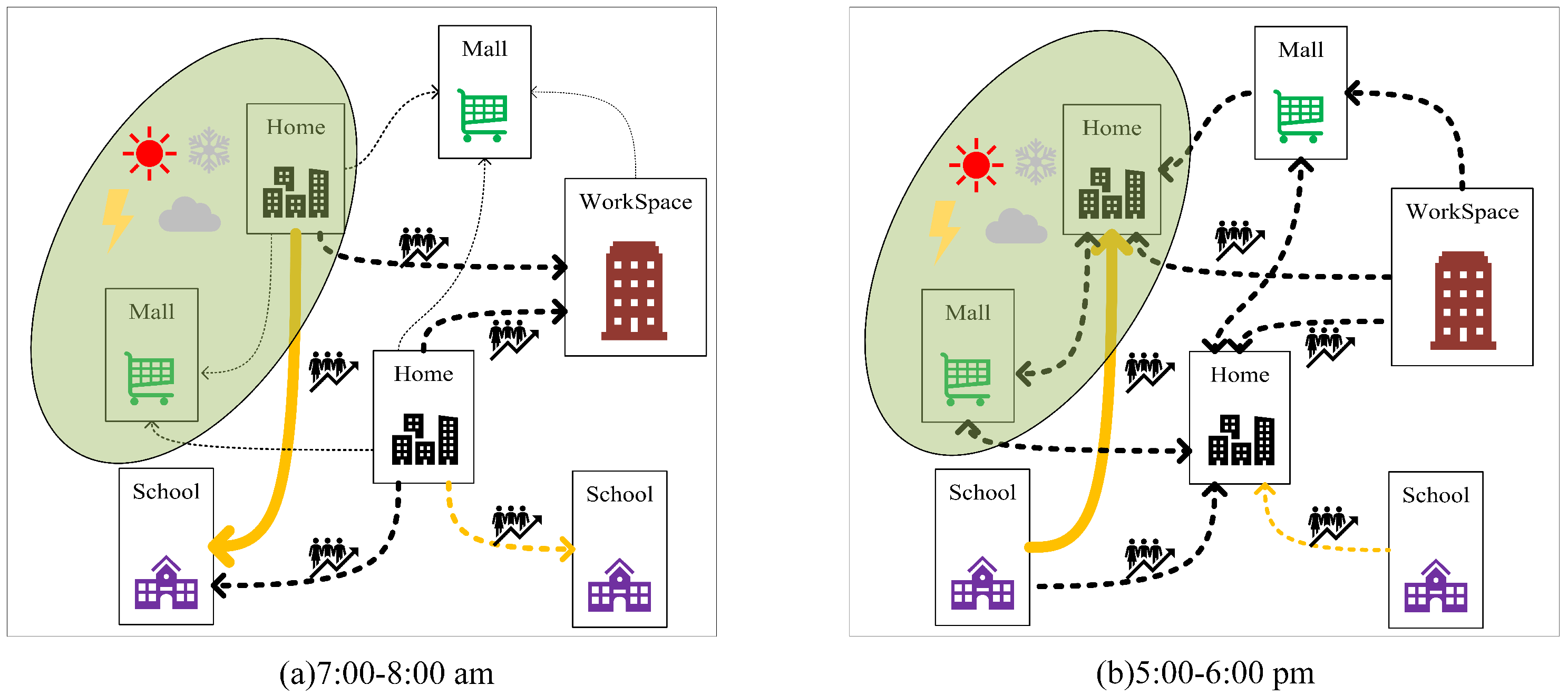
The influence of spatial and temporal features. Between different areas of the city, the urban travel demand of geographically adjacent areas is easily influenced by each other. As shown in Figure 1, in two adjacent areas, such as the residential area and shopping area, the traffic flow has some similarities. The two areas have similar road and business district functions; then at the same time, the demand for taxis in these two areas tends to be similar even if they are geographically distant from each other. For example, if schools are uniformly dismissed at 5 p.m., the demand for taxi rides in the areas near each school will rise significantly and show some similarity. Urban road traffic network and main roads also have a direct impact on the size of the demand. The higher the density of the urban road networks is, with more main roads and larger the road area, the higher the service area and level of operating vehicles will be, and the demand for vehicles from urban residents will increase accordingly.

(2)

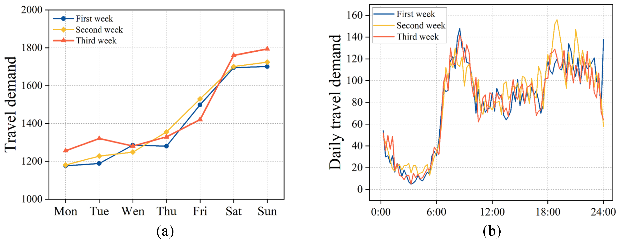
The influence of external features. Some external factors, such as heavy rain, snow, and holidays impact traffic demand. Figure 2, shows that people’s travel demand is higher in sunny weather than in rainy or snowy weather, etc. In Figure 2, it can be seen that people’s travel demand is higher in weather with suitable temperatures than when the temperature is too high or too low. In addition, people’s demand is also influenced by holidays; for example, people will gather in some commercial areas to celebrate the New Year, and the demand will rise on the New Year compared with weekdays. For this reason, this paper also considers the influence of weather and holidays.

To address these challenges, we propose a framework for urban travel demand forecasting based on dynamic multi-view coupled graph convolution. In summary, this paper makes the following contributions:

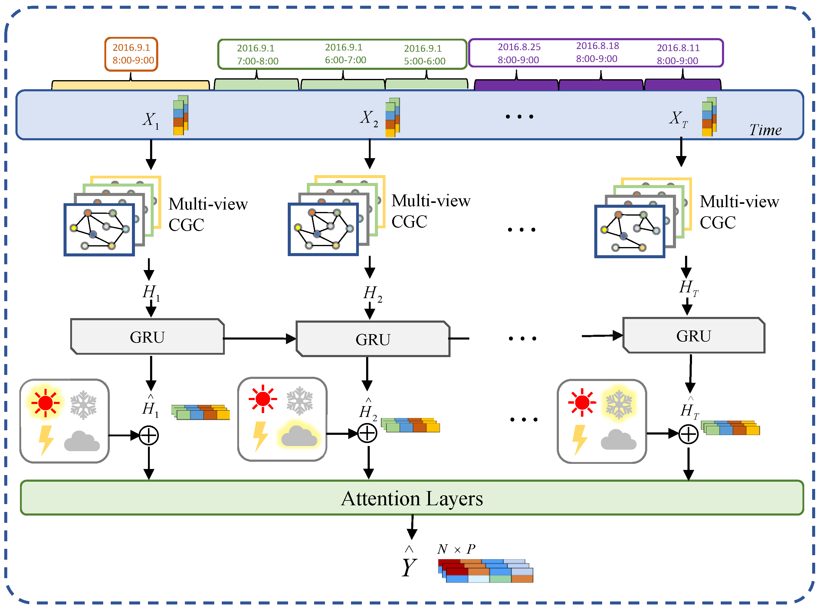
• We propose an urban travel demand forecasting framework based on a dynamic multi-view coupled graph convolutional network, which is able to model the complex spatio-temporal relationships in travel demand data from multiple perspectives.
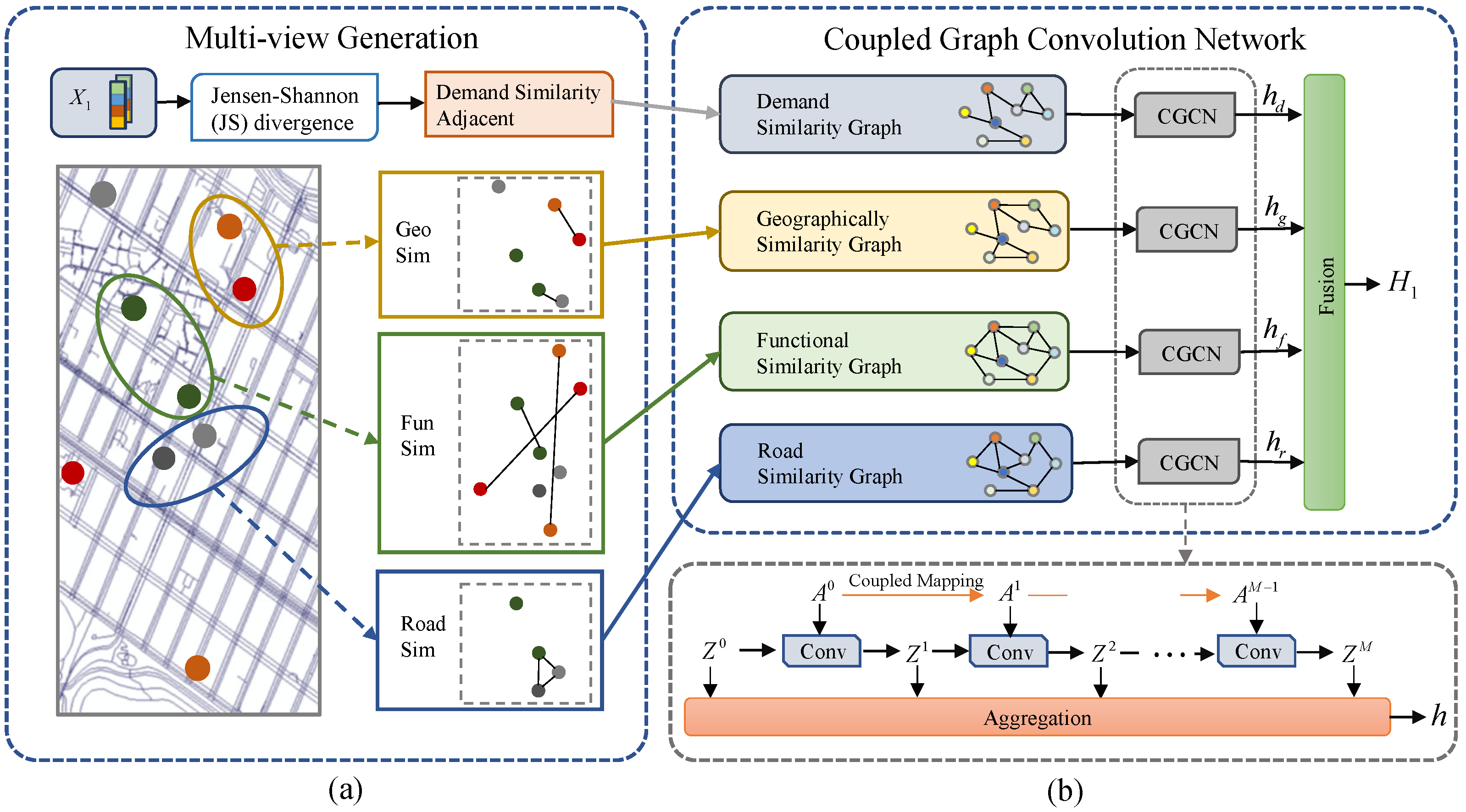
• We propose a method of dynamic demand similarity graph, then fuse geographic similarity graph, functional similarity graph, and road similarity graph to model the dynamic spatio-temporal associations in traffic.
• We conduct experiments on two real datasets, and the results verify the superior performance of our proposed approach compared with state-of-the-art models.

In the following, we first review the related work about urban travel demand prediction in Section 2. We provide the relevant definitions needed for this paper in Section 3. Then we introduce our framework in detail in Section 4. We introduce experimental results and analysis in Section 5. Finally, we summarize our paper in Section 6.

2. Related Work

In this section, we review the related work on urban travel demand forecasting from two aspects: spatio-temporal correlation and urban travel demand forecasting.

2.1. Spatio-Temporal Correlation

Early research methods were mainly based on time series analysis and traditional statistical analysis methods. Since urban travel demand data is a kind of time series data, it is usually processed by time series analysis methods. The most representative one is the autoregressive moving integrated average (ARIMA) model [3], which models univariate traffic condition data streams. There are also some improvement works based on ARIMA models, such as the ARIMI-CARCH [4]. Moreira et al. [5] combine several different time series forecasting techniques such as Time-Varying Poisson Processes [6] and ARIMA models to forecast passenger demand. Li et al. [19] proposed a short-term traffic demand prediction model with the least squares support vector machine (LS-SVM). The main disadvantage of these methods is that they explore the variability of demand time series, but they ignore the effect of spatial correlation of passenger demand between different regions.

In recent years, deep learning has achieved great success in image processing, computer vision, edge computing [20], etc. Many scholars study the use of deep learning methods for urban travel demand forecasting. To capture long-term temporal dependencies, Wu et al. [9] proposed a hybrid deep learning framework, CLTFP, which combines CNN and LSTM for capturing spatio-temporal features. Du et al. [11] used GRU to model the temporal association of hidden states, but GRU is not as powerful and flexible as LSTM. Many scholars divided the area into uniformly sized grids, using CNNs to capture the temporal correlation in the traffic prediction problem [9]. Zhou et al. [21] combined CNNs with attention-based neural networks to achieve multi-step citywide passenger demand forecasting. Ke et al. [22] proposed three H-CNNs (Square, Parity, and Cube H-CNN) and divided the regions into hexagons. However, they usually ignore the modeling of non-Euclidean correlations between regions, which are crucial for urban travel demand forecasting.

The Graph Convolutional Network (GCN) solves the problem of topological data that is difficult to be handled by CNN. Many scholars have started to use GCN to solve traffic-related problems [23,24]. Zhao et al. [14] modeled urban roads as a graph and embedded graph information into GCN. Wang et al. [25] proposed a time-varying graph convolutional network to capture the stability and dynamic spatial correlation of the traffic graph. Li et al. [12] combined diffusion processes with directed road graphs to solve the nonlinear temporal dynamics and complex spatial dependence of road networks. Kong et al. [26] propose a novel region division scheme that considers detailed inter-region relations connected by traffic flux. Zhang et al. [27] used deep spatio-temporal residual networks to predict citywide population movements.

2.2. Urban Travel Demand Forecasting

Among the studies related to traffic demand forecasting, Tang et al. [13] proposed an architecture combining GCN and GRU to capture the spatio-temporal correlation of different regional demand to predict community-level travel demand. Du et al. [11] proposed a dynamically transformed convolutional neural network that uses graph convolution on a dynamically transformed network with the evolutionary flow. Feng et al. [28] proposed a multi-task matrix factorization graph neural network to achieve joint prediction of inflow, outflow, and OD-based ridership demand within a single model framework.

They usually model complex traffic networks as static diagrams, ignoring the importance of constructing similar graphs dynamically over the entire time axis. Wu et al. [29] constructed an adaptive adjacency matrix and preserved the hidden spatial dependencies. Li et al. [15] combined dynamic graphs with predefined graphs to describe the dynamic characteristics of road networks more effectively. Yang et al. [30] proposed an adaptive spatio-temporal graph convolutional network with unique properties of spatio-temporal data to predict fine-grained crowd flows. Ye et al. [31] proposed a novel graph convolution architecture to extract multi-level spatial dependencies adaptively. However, these methods only consider the topological relationship between roads in the composition and ignore other semantic factors that can measure the correlation between roads, such as POI, etc. Jin et al. [17] combined pixel-level features and graph-level features based on the original multi-graph modeling. Chai et al. [16] proposed a multi-graph convolutional neural network model to predict station-level traffic and view the bike-sharing system from a graphical perspective. Geng et al. [18] constructed three graphs of the neighborhood, functional similarity, and traffic connectivity for online demand prediction, respectively. However, most of them do not infer graph connections from the passenger demand data itself.

3. Preliminaries

This subsection briefly introduces the definition of the urban travel demand forecasting problem.

Definition 1.

(Travel Demand): We analyze the urban travel trajectory data, which includes passenger pick-up and drop-off points, etc. We express the departure flow of region i in time interval t as the amount of people’s travel demand.

Definition 2.

(Similarity Graph): The similarity graph is represented as $\mathcal{G}=(V,E,A)$, where each node $v_i$ represents a region, V represents the set of nodes in the graph, E represents the set of edges between regions, i.e., the connectivity between nodes, and A represents the adjacency matrix in graph $\mathcal{G}$. In this paper, we construct similarity graphs from four perspectives, namely dynamic demand similarity graph (represented by ${\mathcal{G}}_D$), functional similarity graph (represented by ${\mathcal{G}}_P$), geographical similarity graph (represented by ${\mathcal{G}}_G$), and road similarity graph (represented by ${\mathcal{G}}_R$), which will be elaborated in Section 4.2.

Definition 3.

(Rush Hour): Rush hour is an important indicator in traffic studies, including morning rush hour and evening rush hour. This paper defines the rush hour as:

$$\mathit{Rush}\mathit{Hour}=\left\{\begin{array}{c}0\mathit{when}t\mathit{in}P\hfill \\ 1\mathit{when}t\mathit{not}\mathit{in}P\hfill \end{array}\right.$$

(1)

where t represents the time interval, and P represents the morning rush hour and evening rush hour. In this paper, it refers to 7 a.m. to 9 a.m. and 5 p.m. to 7 p.m.

Definition 4.

(External Features): The external factors in this paper include mainly weather characteristics and holidays. Weather conditions have a significant impact on urban travel demand. We divide the weather events into five grades: sunny, cloudy, rainy, snowy, and misty. The temperature is scaled to the range of [0, 1] through the minimum and maximum linear normalization. We obtain the holiday situation from the calendar, such as New Year’s Day, etc., connect the data of all external factors into tensors, and input them into the model.

Problem Definition: Given the historical urban travel demand data for the previous p time intervals, we aim to predict the urban travel demand for all regions in the next time interval.

4. Methodology

4.1. DMV-GCN Model

Figure 3, shows the general structure of the model in this paper, which mainly includes three steps: spatial correlation extraction, temporal correlation extraction, and prediction step. Firstly, in spatial correlation extraction, we build a demand similarity graph at each moment. Urban travel demand and time distribution are closely related, and the demand distribution is very different at different moments, so it is necessary to build a demand similarity graph at each moment. In addition, we pre-constructed the geographic similarity graph, the the functional similarity graph, and the road similarity graph and then used the coupled graph convolution to extract features and fuse the output of each similarity graph through the fusion layer to obtain the vector representing the spatial features. Then we use GRU to capture the temporal correlation, and here we combine the external factors (morning and evening rush hour, weather events, etc.). Finally, we get the output of urban travel demand prediction through the attention layer.

4.2. Graph Generation

Dynamic Demand Similarity Graph: Traffic flow data can vary greatly in time series, and capturing this dynamic change is important for urban travel demand forecasting. The previous research methods have focused on mapping all the data stacks of historical moments directly to future demand forecasts, but this cannot simulate the temporal patterns well. We use the historical travel demand data for each region and construct an adjacency matrix at each time interval to capture the similarity of travel demand between regions and adaptively use the time information of the travel demand data. Where the weights of the edge are the similarity of demand patterns between different regions, we capture the similarity of travel demand between regions at each moment.

The dynamic demand similarity graph is established as follows. We construct the demand similarity graph at each moment, which means that the demand similarity graph is different at each moment. We evaluate the demand similarity based on Jensen–Shannon (JS) divergence [32]. JS scatter is widely used to measure the similarity of two probability distributions, and its value range is [0, 1]. The smaller the JS scatter, the higher the similarity between the two regions. The calculation method is as follows:

$$A_d(i,j)=1-JS\left(X_i\parallel X_j\right)$$

(2)

$$\begin{array}{c}\hfill JS\left(X_i\parallel X_j\right)=\frac{1}{2}\sum _{m-1}^M{X}_i\left(m\right)log\frac{2X_i\left(m\right)}{X_i\left(m\right)+X_j\left(m\right)}+\frac{1}{2}\sum _{m-1}^M{X}_j\left(m\right)log\frac{2X_j\left(m\right)}{X_i\left(m\right)+X_j\left(m\right)}\end{array}$$

(3)

where $X_i$ and $X_j$ represent the demand for region i and region j, and M represents the number of features.

Geographically Similarity Graph: According to the first law of geography, the urban travel demand of two geographically adjacent regions shows a certain correlation. We construct the graph by connecting two geographically adjacent regions. The formula for defining the edges in the graph is as follows:

$$A_g(i,j)=\left\{\begin{array}{cc}1,\hfill & \mathrm{region}i\mathrm{and}\mathrm{region}j\mathrm{are}\mathrm{adjacent}\hfill \\ 0,\hfill & \mathrm{otherwise}\hfill \end{array}\right.$$

(4)

Functional Similarity Graph: The demand for urban travel rides is closely related to the distribution of functional areas in the city [18]. Two functionally similar areas have similar demand patterns, even if they are geographically distant from each other. Since POI data can reflect the functionality of regions, we use POI similarity to describe the functional similarity of regions in this paper. We divided the POIs into seven categories (residential areas, schools, recreation, social services, cultural facilities, transportation, and commerce). The similarity is calculated as follows:

$$A_p(i,j)=1-JS\left(P_i\parallel P_j\right)$$

(5)

$$\begin{array}{c}\hfill JS\left(P_i\parallel P_j\right)=\frac{1}{2}\sum _{k=1}^K{P}_i\left(k\right)log\frac{2P_i\left(k\right)}{P_i\left(k\right)+P_j\left(k\right)}+\frac{1}{2}\sum _{k=1}^K{P}_j\left(k\right)log\frac{2P_j\left(k\right)}{P_i\left(k\right)+P_j\left(k\right)}\end{array}$$

(6)

where $P_i,P_j\in {\mathbb{R}}^K$ represents the POI distribution of region i and region j, and K represents the number of POI types.

Road Similarity Graph: Road characteristics (total length of the road, type of road, number of roads, etc.) are also highly correlated with traffic conditions in the region. Similar to the POI similarity calculation, we use the JS divergence to calculate the road similarity between regions. The calculation formula is as follows:

$$A_r(i,j)=1-JS\left(R_i\parallel R_j\right)$$

(7)

$$\begin{array}{c}\hfill JS\left(R_i\parallel R_j\right)=\frac{1}{2}\sum _{l=1}^L{R}_i\left(l\right)log\frac{2R_i\left(l\right)}{R_i\left(l\right)+R_j\left(l\right)}+\frac{1}{2}\sum _{l=1}^L{R}_j\left(l\right)log\frac{2R_j\left(b\right)}{R_j\left(l\right)+R_j\left(l\right)}\end{array}$$

(8)

where $R_i,R_j\in {\mathbb{R}}^L$ represents the road distribution of region i and region j, and L represents the number of road features.

4.3. Spatial Correlation Extraction

Graph convolution network has received wide attention from scholars due to its excellent ability to handle non-Euclidean data. It is widely used in various traffic tasks, such as traffic pattern mining [33], traffic flow prediction [34,35], traffic demand prediction [18], and urban business district excavation [36]. However, in most of the existing studies, graph convolution is implemented on a static adjacency matrix, which cannot accurately reflect the deep-level dependencies between nodes. Inspired by the work [31], we propose multi-view coupled graph convolution, as shown in Figure 4, which uses a coupled graph convolutional network (CGCN) to perform convolution operations to capture the deep spatial correlations between regions. Then we fuse the outputs of multiple views to obtain the final output of spatial correlation extraction.

The propagation law of the coupled graph convolutional network can be expressed as:

$$Z^{(l+1)}=\sum _{i=1}^K{\left(A^{\left(l\right)}\right)}^i{Z}^{\left(l\right)}{W}_i^{\left(l\right)}$$

(9)

where $Z^{\left(l\right)}$ represents the input of layer $l+1$, and $Z^{(l+1)}$ represents the output of layer $l+1$ and the input of layer $l+2$ in the network.

The multilevel graph signal obtained by CGCN is expressed as:

$$\mathbb{Z}=\left\{Z^{\left(1\right)},Z^{\left(2\right)},\dots Z^{\left(M\right)}\right\}$$

(10)

where M represents the total number of graph convolutional layers, and we compute the attention mechanism score by linearly varying:

$${\alpha }^{\left(m\right)}=\frac{exp\left({\widehat{Z}}^{\left(m\right)}{W}_{\alpha }+b_{\alpha }\right)}{{\sum }_{m=1}^{M}exp\left({\widehat{Z}}^{\left(m\right)}{W}_{\alpha }+b_{\alpha }\right)}$$

(11)

$$h=\sum _{m=1}^M{\alpha }^{\left(m\right)}{Z}^{\left(m\right)}$$

(12)

where $W_{\alpha }$ and $b_{\alpha }$ represent the weights and biases in the linear transformation, and ${\widehat{Z}}^{\left(m\right)}$ is the flattened version of $Z^{\left(m\right)}$. Here, ${\alpha }^{\left(m\right)}$ is the attention mechanism score of $Z^{\left(m\right)}$, and h is the final output of $CGCN$, where h can be $h_{d,},h_g,h_f,h_r$.

We input the urban travel demand information and the adjacency matrix of the four similarity graphs into four $CGCN$$\left(CGC{N}_{d,},CGC{N}_g,CGC{N}_f,CGC{N}_r\right)$,

$$\begin{array}{c}{G}_d=\left(A_d,X\right)\stackrel{CGCN}{⟶}{G}_d=\left(A_d,h_d\right)\hfill \\ G_g=\left(A_g,X\right)\stackrel{CGCN}{⟶}{G}_g=\left(A_g,h_g\right)\hfill \\ G_f=\left(A_f,X\right)\stackrel{CGCN}{⟶}{G}_f=\left(A_f,h_f\right)\hfill \\ G_r=\left(A_r,X\right)\stackrel{CGCN}{⟶}{G}_r=\left(A_r,h_r\right)\hfill \end{array}$$

(13)

where $A_{d,},A_g,A_f,A_r$ represent the adjacency matrix, X represents the input feature matrix, and $h_{d,},h_g,h_f,h_r$ represent the output feature matrix.

We fuse the spatial features and update the feature vector of the corresponding node in each graph to a new vector of corresponding multiplicative size.The set of edges in each graph is fused using a merge, so we obtain:

$$G=(A,H)$$

(14)

where H represents the new feature matrix in the fused graph, and A represents the new adjacency matrix.

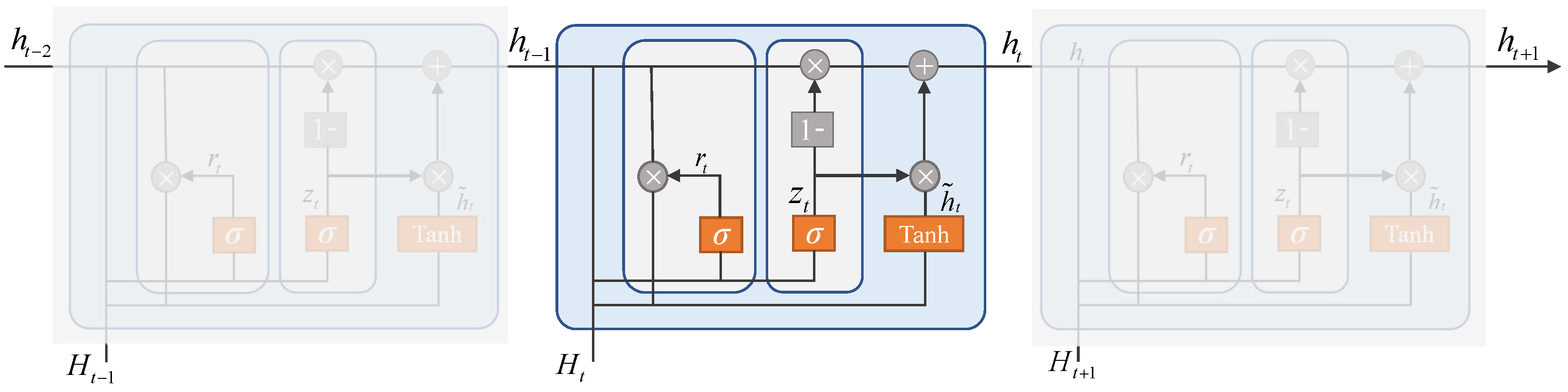
4.4. Temporal Correlation Extraction

Urban travel demand in the city tends to have a strong temporal correlation [13], which is manifested in two main parts: short-term similarity and long-term temporal similarity. Short-term proximity shows that the urban travel demand for rides is affected by the demand in the last few hours, which can be seen from our life scenarios. In addition, there will be more travel demand at night than during the day because buses and subways are closed at night, and people will mostly choose to take a taxi for their night trips for safety reasons. The long-term temporal similarity is shown by the fact that, for example, if a supermarket has a sale on Saturday of each week, the demand in the current area is very similar at that time of the week. The demand on weekdays is different from that on weekends. In Figure 5, we can see that the urban travel demand on weekends is much larger than on weekdays, and the demand at the same time of the same week each week has some similarities. Therefore, in this paper, we select the time slices along the time axis of the first few hours of the moment that needs to be predicted, the same moment of the first few days and the same moment of the same week of the first few weeks, and splice them into a time series $S=\left\{S_1,S_2,\dots S_{q,\dots }{S}_T\right\}$.

GRU (Gates Recurrent Unit) is a kind of RNN (Recurrent Neural Network), and like LSTM (Long-Short Term Memory), it was proposed to solve the problems of long-term memory and gradient in back propagation. However, GRU has a simpler model compared with LSTM, as shown in Figure 6. It is easier to compute, and the experimental results are similar to LSTM. So in this paper, we use GRU to extract temporal correlation:

$${\widehat{H}}_t^i=GRU\left(H_t^i,{\widehat{H}}_{t-1}^i\right)$$

(15)

where $H_t^i$ represents the output of the multi-view coupled graph convolution of node i at time interval t, ${\widehat{H}}_t^i\in {\mathbb{R}}^{d_H}$ represents the hidden state of region i at time interval t, and $d_H$ represents the number of hidden units.

All nodes of GRU share the same parameters. We denote the output of the hidden state of all nodes by $U=\left[{\widehat{H}}_1,{\widehat{H}}_2,\dots ,{\widehat{H}}_T\right]$, where ${\widehat{H}}_t\in {\mathbb{R}}^{N\times d_H}$. Then we compute the attention score between U and the external feature $E=\left\{e_1,e_{2,\dots ,}{e}_T\right\}$, where $e_i\in {\mathbb{R}}^{N\times d_e}$, $d_e$ is denoted as the number of external features. Finally, we use temporal attention to dynamically capture the temporal correlation:

$$\alpha =softmax\left(ReLU\left(U{W}_S+E{W}_E+b_{\alpha }\right)\right)$$

(16)

where $W_S\in {\mathbb{R}}^{d_H\times 1}$, $W_E\in {\mathbb{R}}^{d_e\times 1}$, $b_{\alpha }\in {\mathbb{R}}^T$ is a learnable parameter, and $\alpha \in {\mathbb{R}}^T$ is the temporal attention score vector, which represents the importance distribution of different historical time intervals on the target interval. Then the temporal correlation extraction can be expressed as:

$$\widehat{Y}=\sum _{i=1}^T{\alpha }_i·{\widehat{H}}_i$$

(17)

5. Experiments

5.1. Datasets

We conduct experiments on two real datasets. The experimental dataset includes: (1) NYC-taxi-2016. It refers to the public dataset of New York City taxis. This dataset uses data from January to June 2016 in Manhattan, New York City. We divide the dataset according to 15-min intervals, which removes data items where the taxi travel distance is zero. (2) The NYC-taxi-2019. It is the same as above. This dataset uses the data from July to December 2019 and is also divided into 15-min intervals, and the data items with a moving distance of 0 are also removed. We calculate the total number of taxi pick-up points in each area at each time interval as the travel demand. We acquire and analyze POI data and road feature data from maps. POI data mainly includes seven categories: residential areas, schools, recreation, social services, cultural facilities, transportation, and commerce; road characteristics mainly include road type(primary, secondary, trunk, tertiary, service, motorway, residential, cycleway, footway) and road section lengths; and weather data includes sunny, rainy, cloudy, snowy, and misty days.

5.2. Experiment Settings

Valuation Metrics

We consider the urban travel demand forecasting task as a regression problem, and in this paper, we use Root Mean Square Error (RMSE), Mean Absolute Error (MAE), and Mean Absolute Percentage Error (MAPE) as evaluation metrics.

• RMSE: It is used to measure the deviation between the predicted value and the true value, defined as:

  $$RMSE=\sqrt{\frac{1}{N}{\displaystyle \sum _{i=1}^N}{\left(Y_i-{\widehat{Y}}_i\right)}^2}$$

  (18)
• MAE: It is used to measure the mean of absolute error, defined as:

  $$MAE=\frac{1}{N}\sum _{i=1}^N\left|Y_i-{\widehat{Y}}_i\right|$$

  (19)
• MAPE: It is used to measure the percentage of predicted value to true value, defined as:

  $$MAPE=\frac{100\%}{N}\sum _{i=1}^N\left|\frac{Y_i-{\widehat{Y}}_i}{Y_i}\right|$$

  (20)

Implementation Details

The dataset is first divided into 60%, 20%, and 20%, representing the training, validation, and test sets, respectively. The model is optimized by back propagation. The model learning rate is set to 0.001, and the Adam optimizer is applied for optimization. The input time slice length T set in this paper is 12, so the dimension of the input is $12\times 2\times N$. N represents the number of nodes, and the predicted time lengths are 1, 2, 3, and 4, representing 15 min, 30 min, 45 min, and 60 min, respectively. The MAE is used as the loss function for training.

Baselines methods

We compare our model with the following seven baseline models:

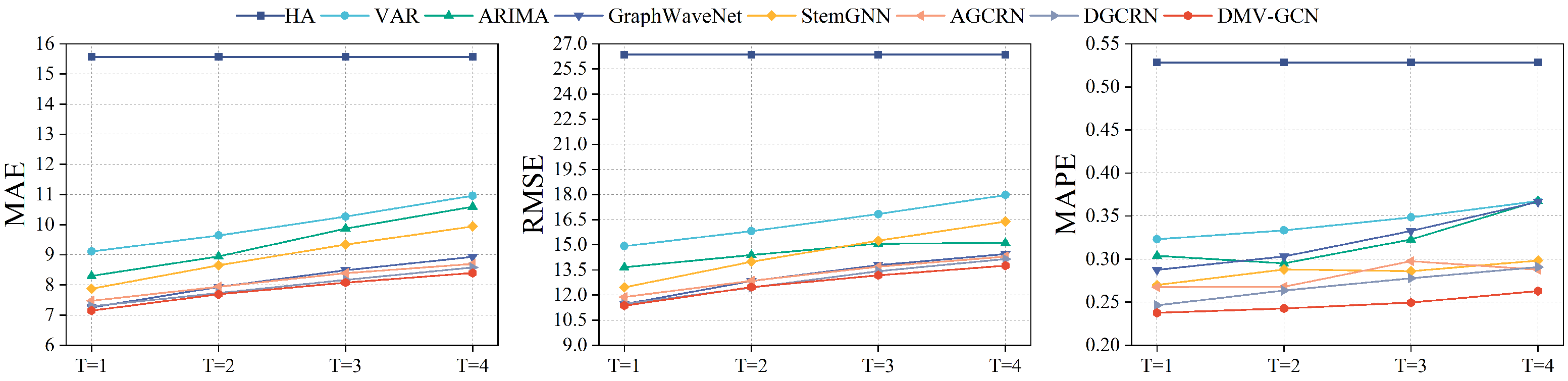
• HA: The historical average of the predicted time step is used as the predicted value.
• VAR: Vector autoregression for time series forecasting.
• ARIMA: Combining autoregressive and moving average models for time series forecasting.
• Graph WaveNet [29]: Graph convolution with adaptive adjacency matrices combines graph convolution operations and null causal convolution.
• StemGNN [37]: A spectroscopic time map neural network that jointly captures inter-sequence correlations and time dependence in the spectral domain.
• AGCRN [38]: Adaptive graphs are used to learn GRU in combination with graph convolution and node adaptive parameter learning.
• DGCRN [15]: The dynamic adjacency matrix is progressively generated from the hypernetwork, iterating in parallel with the RNN.

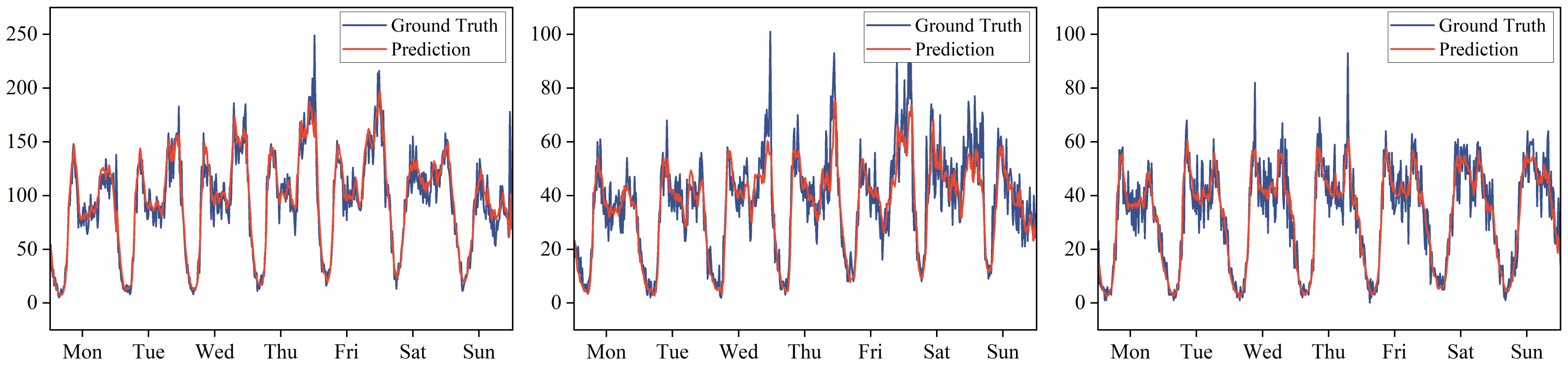
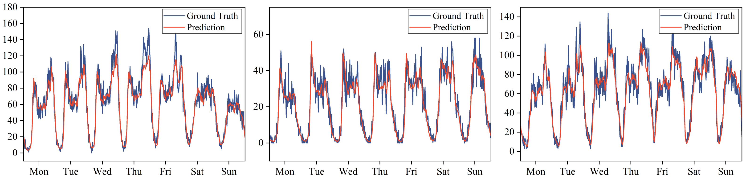
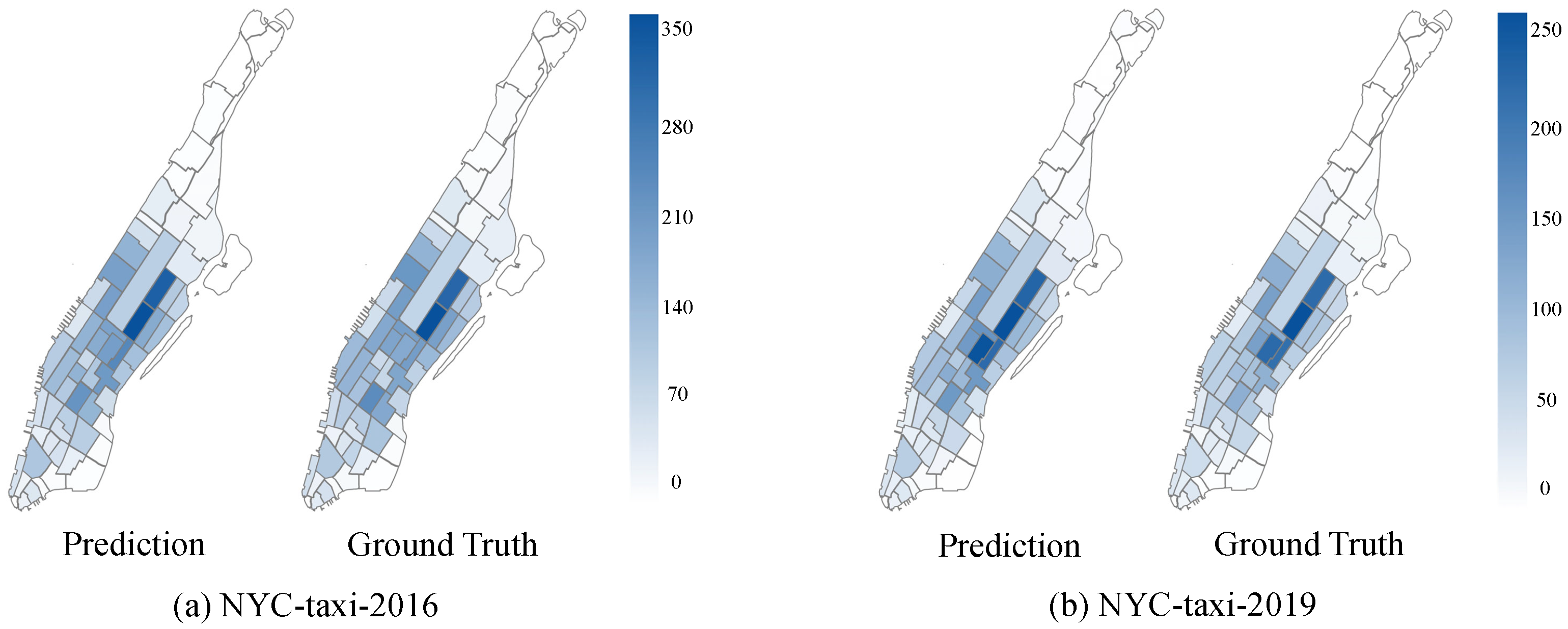
Experiment Results

Table 1. Comparison of experimental results on the NYC-taxi-2016 datasets.

Model	MAE				RMSE				MAPE
	T = 1	T = 2	T = 3	T = 4	T = 1	T = 2	T = 3	T = 4	T = 1	T = 2	T = 3	T = 4
HA	15.5656	15.5656	15.5656	15.5656	26.3609	26.3609	26.3609	26.3609	52.85%	52.85%	52.85%	52.85%
VAR	9.1140	9.6430	10.2674	10.9622	14.9206	15.8139	16.8368	17.9714	32.31%	33.35%	34.86%	36.74%
ARIMA	8.3027	8.9496	9.8732	10.5988	13.6551	14.3841	15.0756	15.1062	30.38%	29.51%	32.28%	36.76%
GraphWaveNET	7.2558	7.9336	8.4908	8.9350	11.4538	12.8381	13.7841	14.4507	28.77%	30.32%	33.28%	36.65%
StemGNN	7.8737	8.6559	9.3412	9.9432	12.4606	13.9908	15.2511	16.3861	26.99%	28.81%	28.59%	29.83%
AGCRN	7.4766	7.9428	8.3931	8.6966	11.8761	12.8451	13.6885	14.2983	26.74%	26.79%	29.76%	28.79%
DGCRN	7.2919	7.7324	8.1710	8.5788	11.4688	12.4485	13.4257	14.1501	24.65%	26.36%	27.78%	29.09%
DMV-GCN	7.1527	7.6892	8.0813	8.3983	11.3687	12.4712	13.1819	13.7580	23.76%	24.28%	24.96%	26.30%

and

Table 2. Comparison of experimental results on the NYC-taxi-2019 datasets.

Model	MAE				RMSE				MAPE
	T = 1	T = 2	T = 3	T = 4	T = 1	T = 2	T = 3	T = 4	T = 1	T = 2	T = 3	T = 4
HA	9.2981	9.2981	9.2981	9.2981	16.4961	16.4961	16.4961	16.4961	60.86%	60.86%	60.86%	60.86%
VAR	6.9041	7.1414	7.4254	7.7397	12.6623	13.1045	13.6094	14.1602	45.46%	47.19%	49.40%	52.02%
ARIMA	6.1517	6.9229	7.3199	7.5304	10.3807	11.2033	11.4912	13.2935	40.73%	49.87%	53.42%	46.22%
GraphWaveNet	5.7631	6.4184	6.9606	7.4902	9.5184	10.8770	11.9056	12.8824	30.77%	32.75%	35.14%	37.33%
StemGNN	5.6223	5.7510	6.0954	6.4572	9.8931	10.2711	11.0161	11.7550	34.06%	34.61%	35.65%	38.06%
AGCRN	5.6107	5.9134	6.1992	6.4304	9.3818	10.0416	10.5704	10.9811	32.16%	31.78%	33.84%	33.99%
DGCRN	5.4037	5.8837	6.3532	6.9375	8.8506	9.8173	10.6640	11.6736	32.47%	34.12%	35.96%	37.63%
DMV-GCN	5.3452	5.7451	6.0053	6.2584	8.8454	9.6062	10.1059	10.6034	29.41%	30.10%	30.85%	32.04%

show the prediction performance of our model and the baseline model on both datasets. It can be seen that our DMV-GCN model achieves the best performance on both datasets. Specifically, HA, VAR, and ARIMA perform poorly because they have limited ability to model complex dependencies of spatio-temporal data and are less efficient in mining sufficient information. Compared with traditional machine methods, the deep-learning-based model has better performance. Graph WaveNet uses an adaptive adjacency matrix to model dynamic spatio-temporal dependencies and introduces a null causal one-dimensional convolution model to replace the RNN model. StemGNN transfers the spatio-temporal domain to the frequency domain by discrete Fourier transform and graph Fourier transform and captures the spatio-temporal dependencies in the frequency domain simultaneously. AGCRN proposes a data adaptive graph generation module to infer the interdependence between different traffic time series automatically. However, they all have difficulties in modeling dynamic spatio-temporal dependencies on each time slice. DGCRN uses RNN to model spatio-temporal dependencies, which loses some global temporal information although it usually ignores the influence of external factors on urban travel demand. Overall, our DMV-GCN model is able to capture the different effects of different external factors on urban travel demand while combining dynamic demand similarity graphs and three semantic similarity graphs. As a result, DMV-GCN achieves the best performance among all methods, which further demonstrates the superior performance of DMV-GCN in modeling the multi-scale spatio-temporal correlation of urban travel demand.

Time-Slice Length Analysis

To investigate the effect of time slice length on model performance, experiments are conducted in this section to predict time slices of different lengths. In this paper, we set the time slice length as 15 min, 30 min, 45 min, and 60 min, respectively. As shown in Figure 7 and Figure 8, with the increase of time slice length, the uncertainty factors affecting traffic increase, and the overall effectiveness of the model shows a decreasing trend. This indicates that the excessively long time granularity reduces the ability of the model to capture the characteristics of traffic conditions and leads to a slight decrease in performance. Moreover, we can see that the longer the time slice length, the better the effectiveness of our proposed DMV-GCN model relative to other baseline models, which indicates that the robustness of the model is better.

Ablation Study

In order to further illustrate the effectiveness of different components, we conduct ablation experiments in this subsection. We design four variants, respectively removing the demand similarity graph, the geographic similarity graph, the functional similarity graph, and the road similarity graph from the DMV-GCN, and other settings are the same as DMV-GCN. We name these four variants as w/o dynamic, w/o geo, w/o poi, and w/o road. Figure 9 and Figure 10 show the performance comparison of DMV-GCN with different variants. The w/o dynamic has the worst effect, which shows that it is very necessary and effective for us to dynamically construct the demand similarity graph, and the other three variants also have a poor effect, which shows that the distribution of functional areas, geographical location, and road characteristics of the region have a greater influence on travel demand. It can be seen that the DMV-GCN is higher than the four variants at all indicators, which shows the validity of each of our proposed components.

5.3. Visualization

To further test the capability of our model in predicting urban travel demand, we compared the predicted results with the true values. We randomly selected three areas. Figure 11 and Figure 12 show the visualization results of the travel demand of these three areas on the two datasets. We take 15 min as the basic unit; blue represents the prediction result of our model, and orange represents the real value. It can be seen that the prediction effect of our model on the two datasets is very similar to the real value, and the travel demand has obvious morning and evening peak characteristics. In addition, to more visually demonstrate the practical application of our model, we constructed heat maps showing the travel demand for all regions at our selected times. On the NYC-taxi-2016 dataset, we selected 25 May 2016 from 18:00 to 18:15, and on the NYC-taxi-2019 dataset, we selected 2019 25 November 2016 from 18:00 to 18:15. As shown in Figure 13, the shades of the heat map color indicate the high or low regional travel demand. We can see that the colors of the prediction map and the true value map are very close, which indicates that our model can provide very accurate prediction results.

6. Conclusions

In this paper, we propose a new dynamic multi-view coupled graph convolution model named DMV-GCN to predict urban travel demand more effectively. To capture deep spatio-temporal correlations, we dynamically construct demand similarity graphs at each moment with the weights of edges learned from urban travel demand data. Combining the predefined geographic similarity graph, the functional similarity graph, and the road similarity graph, we fuse them by using coupled graph convolution and combine GRU to capture spatio-temporal correlations. Finally, we fuse the external environmental factors for urban travel demand prediction. We evaluated our model on two real-world datasets, and the results validated our model due to state-of-the-art methods. However, the limitation of this method is that it has high requirements on the dataset. We consider more factors, such as the traffic flow data, road data, POI data, and weather data, in our method. Now such datasets with sufficient information are very limited, which affect applicability and generalization ability of our method. In the future, we will improve the structure of various parts of our model and increase its generality in different scenarios to adapt to more datasets.

References

1. Han, X.; Shen, G.; Yang, X.; Kong, X. Congestion recognition for hybrid urban road systems via digraph convolutional network. Transp. Res. Part Emerg. Technol. 2020, 121, 102877. [Google Scholar] [CrossRef]
2. Kong, X.; Zhu, B.; Shen, G.; Chekole Workneh, T.; Ji, Z.; Chen, Y.; Liu, Z. Spatial-Temporal-Cost Combination based Taxi Driving Fraud Detection for Collaborative Internet of Vehicles. IEEE Trans. Ind. Inform. 2021, 18, 3426–3436. [Google Scholar] [CrossRef]
3. Cetin, M.; Comert, G. Short-term traffic flow prediction with regime switching models. Transp. Res. Rec. 2006, 1965, 23–31. [Google Scholar] [CrossRef]
4. Chen, C.; Hu, J.; Meng, Q.; Zhang, Y. Short-time traffic flow prediction with ARIMA-GARCH model. In Proceedings of the 2011 IEEE Intelligent Vehicles Symposium (IV), Baden-Baden, Germany, 5–9 June 2011; pp. 607–612. [Google Scholar]
5. Moreira-Matias, L.; Gama, J.; Ferreira, M.; Mendes-Moreira, J.; Damas, L. Predicting taxi–passenger demand using streaming data. IEEE Trans. Intell. Transp. Syst. 2013, 14, 1393–1402. [Google Scholar] [CrossRef] [Green Version]
6. Ihler, A.; Hutchins, J.; Smyth, P. Adaptive event detection with time-varying poisson processes. In Proceedings of the 12th ACM SIGKDD International Conference on Knowledge Discovery and Data Mining, Philadelphia, PA, USA, 20–23 August 2006; pp. 207–216. [Google Scholar]
7. Zhang, L.; Liu, Q.; Yang, W.; Wei, N.; Dong, D. An improved k-nearest neighbor model for short-term traffic flow prediction. Procedia-Soc. Behav. Sci. 2013, 96, 653–662. [Google Scholar] [CrossRef] [Green Version]
8. Wu, Y.; Tan, H.; Qin, L.; Ran, B.; Jiang, Z. A hybrid deep learning based traffic flow prediction method and its understanding. Transp. Res. Part Emerg. Technol. 2018, 90, 166–180. [Google Scholar] [CrossRef]
9. Wu, Y.; Tan, H. Short-term traffic flow forecasting with spatial-temporal correlation in a hybrid deep learning framework. arXiv 2016, arXiv:1612.01022. [Google Scholar]
10. Liao, B.; Zhang, J.; Wu, C.; McIlwraith, D.; Chen, T.; Yang, S.; Guo, Y.; Wu, F. Deep sequence learning with auxiliary information for traffic prediction. In Proceedings of the24th ACM SIGKDD International Conference on Knowledge Discovery & Data Mining, London, UK, 19–23 August 2018; pp. 537–546. [Google Scholar]
11. Du, B.; Hu, X.; Sun, L.; Liu, J.; Qiao, Y.; Lv, W. Traffic demand prediction based on dynamic transition convolutional neural network. IEEE Trans. Intell. Transp. Syst. 2020, 22, 1237–1247. [Google Scholar] [CrossRef]
12. Li, Y.; Yu, R.; Shahabi, C.; Liu, Y. Diffusion convolutional recurrent neural network: Data-driven traffic forecasting. arXiv 2017, arXiv:1707.01926. [Google Scholar]
13. Tang, J.; Liang, J.; Liu, F.; Hao, J.; Wang, Y. Multi-community passenger demand prediction at region level based on spatio-temporal graph convolutional network. Transp. Res. Part Emerg. Technol. 2021, 124, 102951. [Google Scholar] [CrossRef]
14. Zhao, L.; Song, Y.; Zhang, C.; Liu, Y.; Wang, P.; Lin, T.; Deng, M.; Li, H. T-gcn: A temporal graph convolutional network for traffic prediction. IEEE Trans. Intell. Transp. Syst. 2019, 21, 3848–3858. [Google Scholar] [CrossRef] [Green Version]
15. Li, F.; Feng, J.; Yan, H.; Jin, G.; Jin, D.; Li, Y. Dynamic graph convolutional recurrent network for traffic prediction: Benchmark and solution. arXiv 2021, arXiv:2104.14917. [Google Scholar] [CrossRef]
16. Chai, D.; Wang, L.; Yang, Q. Bike flow prediction with multi-graph convolutional networks. In Proceedings of the26th ACM SIGSPATIAL International Conference on Advances in Geographic Information Systems, Seattle, WA, USA, 6–9 November 2018; pp. 397–400. [Google Scholar]
17. Jin, G.; Cui, Y.; Zeng, L.; Tang, H.; Feng, Y.; Huang, J. Urban ride-hailing demand prediction with multiple spatio-temporal information fusion network. Transp. Res. Part Emerg. Technol. 2020, 117, 102665. [Google Scholar] [CrossRef]
18. Geng, X.; Li, Y.; Wang, L.; Zhang, L.; Yang, Q.; Ye, J.; Liu, Y. Spatiotemporal multi-graph convolution network for ride-hailing demand forecasting. In Proceedings of the AAAI Conference On Artificial Intelligence, Honolulu, HI, USA, 27 January–1 February 2019; Volume 33, pp. 3656–3663. [Google Scholar]
19. Li, Y.; Lu, J.; Zhang, L.; Zhao, Y. Taxi booking mobile app order demand prediction based on short-term traffic forecasting. Transp. Res. Rec. 2017, 2634, 57–68. [Google Scholar] [CrossRef]
20. Kong, X.; Duan, G.; Hou, M.; Shen, G.; Wang, H.; Yan, X.; Collotta, M. Deep Reinforcement Learning based Energy Efficient Edge Computing for Internet of Vehicles. IEEE Trans. Ind. Inform. 2022, 18, 6308–6316. [Google Scholar] [CrossRef]
21. Zhou, X.; Shen, Y.; Zhu, Y.; Huang, L. Predicting multi-step citywide passenger demands using attention-based neural networks. In Proceedings of the Eleventh ACM International Conference on Web Search and Data Mining, Los Angeles, CA, USA, 5–9 February 2018; pp. 736–744. [Google Scholar]
22. Ke, J.; Yang, H.; Zheng, H.; Chen, X.; Jia, Y.; Gong, P.; Ye, J. Hexagon-based convolutional neural network for supply-demand forecasting of ride-sourcing services. IEEE Trans. Intell. Transp. Syst. 2018, 20, 4160–4173. [Google Scholar] [CrossRef]
23. Song, C.; Lin, Y.; Guo, S.; Wan, H. Spatial-temporal synchronous graph convolutional networks: A new framework for spatial-temporal network data forecasting. In Proceedings of the AAAI Conference on Artificial Intelligence, New York, NY, USA, 7–12 February 2020; Volume 34, pp. 914–921. [Google Scholar]
24. Zhang, Q.; Chang, J.; Meng, G.; Xiang, S.; Pan, C. Spatio-temporal graph structure learning for traffic forecasting. In Proceedings of the AAAI Conference on Artificial Intelligence, New York, NY, USA, 7–12 February 2020; Volume 34, pp. 1177–1185. [Google Scholar]
25. Wang, Y.; Fang, S.; Zhang, C.; Xiang, S.; Pan, C. TVGCN: Time-variant graph convolutional network for traffic forecasting. Neurocomputing 2022, 471, 118–129. [Google Scholar] [CrossRef]
26. Kong, X.; Chen, Q.; Hou, M.; Rahim, A.; Ma, K.; Xia, F. RMGen: A Tri-Layer Vehicular Trajectory Data Generation Model Exploring Urban Region Division and Mobility Pattern. IEEE Trans. Veh. Technol. 2022. [Google Scholar] [CrossRef]
27. Zhang, J.; Zheng, Y.; Qi, D.; Li, R.; Yi, X.; Li, T. Predicting citywide crowd flows using deep spatio-temporal residual networks. Artif. Intell. 2018, 259, 147–166. [Google Scholar] [CrossRef] [Green Version]
28. Feng, S.; Ke, J.; Yang, H.; Ye, J. A multi-task matrix factorized graph neural network for co-prediction of zone-based and OD-based ride-hailing demand. IEEE Trans. Intell. Transp. Syst. 2021, 23, 5704–5716. [Google Scholar] [CrossRef]
29. Wu, Z.; Pan, S.; Long, G.; Jiang, J.; Zhang, C. Graph wavenet for deep spatial-temporal graph modeling. In Proceedings of the 28th International Joint Conference on Artificial Intelligence, Macao, China, 10–16 August 2019; pp. 1907–1913. [Google Scholar]
30. Yang, X.; Zhu, Q.; Li, P.; Chen, P.; Niu, Q. Fine-grained predicting urban crowd flows with adaptive spatio-temporal graph convolutional network. Neurocomputing 2021, 446, 95–105. [Google Scholar] [CrossRef]
31. Ye, J.; Sun, L.; Du, B.; Fu, Y.; Xiong, H. Coupled layer-wise graph convolution for transportation demand prediction. In Proceedings of the AAAI Conference on Artificial Intelligence, Virtually, 2–9 February 2021; Volume 35, pp. 4617–4625. [Google Scholar]
32. Lin, J. Divergence measures based on the Shannon entropy. IEEE Trans. Inf. Theory 1991, 37, 145–151. [Google Scholar] [CrossRef] [Green Version]
33. Shen, G.; Zhu, D.; Chen, J.; Kong, X. Motif discovery based traffic pattern mining in attributed road networks. Knowl. Based Syst. 2022, 250, 109035. [Google Scholar] [CrossRef]
34. Liu, L.; Zhen, J.; Li, G.; Zhan, G.; He, Z.; Du, B.; Lin, L. Dynamic spatial-temporal representation learning for traffic flow prediction. IEEE Trans. Intell. Transp. Syst. 2020, 22, 7169–7183. [Google Scholar] [CrossRef]
35. Pian, W.; Wu, Y.; Qu, X.; Cai, J.; Kou, Z. Spatial-temporal dynamic graph attention networks for ride-hailing demand prediction. arXiv 2020, arXiv:2006.05905. [Google Scholar]
36. Shen, G.; Zhao, Z.; Kong, X. GCN2CDD: A commercial district discovery framework via embedding space clustering on graph convolution networks. IEEE Trans. Ind. Inform. 2021, 18, 356–364. [Google Scholar] [CrossRef]
37. Cao, D.; Wang, Y.; Duan, J.; Zhang, C.; Zhu, X.; Huang, C.; Tong, Y.; Xu, B.; Bai, J.; Tong, J.; et al. Spectral temporal graph neural network for multivariate time-series forecasting. Adv. Neural Inf. Process. Syst. 2020, 33, 17766–17778. [Google Scholar]
38. Bai, L.; Yao, L.; Li, C.; Wang, X.; Wang, C. Adaptive graph convolutional recurrent network for traffic forecasting. Adv. Neural Inf. Process. Syst. 2020, 33, 17804–17815. [Google Scholar]
Figure 1. An example of different relationships among regions.
Electronics 11 02620 g001
Figure 2. The influence of weather events.
Electronics 11 02620 g002
Figure 3. The overall framework of the DMV-GCN model.
Electronics 11 02620 g003
Figure 4. Multi-view coupled graph convolutional network.
Electronics 11 02620 g004
Figure 5. (a) Total daily travel demand for a region for three consecutive weeks; (b) daily travel demand on Monday of each week for three consecutive weeks.
Electronics 11 02620 g005
Figure 6. The basic unit of the GRU network.
Electronics 11 02620 g006
Figure 7. Comparison of the effect of different time-slice on NYC-taxi-2016.
Electronics 11 02620 g007
Figure 8. Comparison of the effect of different time-slice on NYC-taxi-2019.
Electronics 11 02620 g008
Figure 9. Performance comparison between DMV-GCN and its variant models on NYC-taxi-2016.
Electronics 11 02620 g009
Figure 10. Performance comparison between DMV-GCN and its variant models on NYC-taxi-2019.
Electronics 11 02620 g010
Figure 11. Visualization of travel demand for one week in three regions on NYC-taxi-2016(6/13–6/19).
Electronics 11 02620 g011
Figure 12. Visualization of travel demand for one week in three regions on NYC-taxi-2019(12/9–12/15).
Electronics 11 02620 g012
Figure 13. Visualization of travel demand for 15 min in all regions on two datasets.
Electronics 11 02620 g013