Segmentation of Spectral Plant Images Using Generative Adversary Network Techniques

Abstract

The spectral image analysis of complex analytic systems is usually performed in analytical chemistry. Signals associated with the key analytics present in an image scene are extracted during spectral image analysis. Accordingly, the first step in spectral image analysis is to segment the image in order to extract the applicable signals for analysis. In contrast, using traditional methods of image segmentation in chronometry makes it difficult to extract the relevant signals. None of the approaches incorporate contextual information present in an image scene; therefore, the classification is limited to thresholds or pixels only. An image translation pixel-to-pixel (p2p) method for segmenting spectral images using a generative adversary network (GAN) is presented in this paper. The p2p GAN forms two neuronal models. During the production and detection processes, the representation learns how to segment ethereal images precisely. For the evaluation of the results, a partial discriminate analysis of the least-squares method was used to classify the images based on thresholds and pixels. From the experimental results, it was determined that the GAN-based p2p segmentation performs the best segmentation with an overall accuracy of 0.98 ± 0.06. This result shows that image processing techniques using deep learning contribute to enhanced spectral image processing. The outcomes of this research demonstrated the effectiveness of image-processing techniques that use deep learning to enhance spectral-image processing.

1. Introduction

Spectral imaging is imaging that uses multiple bands across the electromagnetic spectrum and is commonly deployed in the area of analytical chemistry. Spectral imaging is deployed for investigating spatially dispersed features of complicated analytical systems, e.g., micro plastic detection, fish and meat analyses, pharmaceutical formulations, and so on [1]. Spectral imaging gathers images and spectroscopy data. Spectral analysis records the physicochemical properties of samples, while imaging captures the spatial context of the photographed scene. Spectral imaging provides rich spectral and spatial information that is useless on its own, and conclusions must be drawn from the data after appropriate data processing [2]. The major spectral image-processing operations include radiometric correction, preprocessing, segmentation, and data modeling [3]. Radiometric correction is performed on all images using the same white and dark references, while preprocessing steps vary according to the images. For example, de-noising can be performed on the noisy images, as well as spectral normalization and derivatives when there are additive and multiplicative effects in the pixels. Radiometric correction and preprocessing yield high-quality spectral images; then, the model-training data must be retrieved [4,5]. In the spectral images, the segmentation of the images plays a very crucial role, as the spectral images consist of spatial information as well as spectral information; thus, the processing cost of these images is higher in comparison to the pixel-based images. So, poor segmentation can increase the image-processing cost and the pixels from the training stage may contain data unrelated to the region of interest, consequently complicating or further worsening the data modeling. This paper presents the GAN-based spectral image segmentation method that ensures effective segmentation by providing two-staged image segmentation. In the first stage, the segmentation is attained, while the second stage consists of the verification of the segmented image.

Multiple authors have presented different methods for spectral picture segmentation in chemometrics. A standard Otsu-based picture segmentation algorithm that uses some selected contrasting-band images is deployed in [6]. It is shown that if only a few spectral images are to be analyzed, a physical area of notice assortment can be performed by drawing polygons. In addition, pixel-based classifiers can be trained to segment spectral images based on pixels in more complex situations. Spectral image segmentation can be challenging with threshold- and Otsu-based methods because of the presence of several analyses with similar spectral signatures in the imaged scene. The spatial context provided by the imaged scene combined with the spectral signals can be crucial to deriving efficient segmentation, since different analyses may have the same spectral signals but can be viewed from dissimilar places in the image panorama.

In most instances, ethereal image segmentation with modeling is pixel-based, which ignores how images are arranged in space. However, some recent studies are providing insights into using spatial information and combining spectral information to produce better results [6]. A well-proven butterfly technique for spectral picture segmentation, for example, makes use of spectral information in both topological and latent spaces. A new pixel-based classifier could be trained by extracting textual information. According to a recent study, the spectral images with average (in bands) spectra can be stacked with spectral planes. Another recent study recommends dividing spectral band pictures into horizontal, vertical, diagonal, and approximation components and to train pixels based on spectral planes and pair them with spectral planes’ classifiers using 2D-wavelet decomposition. Another study recently highlighted a method for utilizing posterior analysis, which was proposed for analyzing spatial contexts to assess the quality of predicted spectrum maps [7]. The primary issue with the existing spectral imaging spatial-spectral analysis (segmentation/modeling) methods is that they need to remove spatial and spectral information in sequence separately. Furthermore, some methods simply extract spatial data, which then necessitates a further modeling phase to make use of the collected data. Various strategies for understanding both the geographical context and spectral patterns are now available.

Deep Learning (DL) algorithms are used in several domains, including computer vision. In order to conduct efficient modeling, convolution-based DL models, such as those based on 2D and 3D convolutions, are often used for extracting deep contextual and band-related information. DL offers several methods to segment images with the spatial context and banding information of customized techniques. There are also options for utilizing an instance and semantic segmentation. Convolution filters use a collection of training images to learn the segmentation problem, and the learned weights to segment additional test images, making the fully connected Convolution Neural Network (CNN) the first and easiest to build solution [8]. The segmentation of biomedical images has been made easier with the use of DL architectures based on expanding and contracting routes [9]. The new design has been dubbed the U-net because the network had a U-shaped appearance owing to a series of down-sampling and up-sampling convolutions. As a result, several new techniques have been introduced, including Deep Lab, which is based on atrous or dilated convolutions. For image translation problems, generative models have recently been developed in addition to classic convolution networks [10]. Translating satellite images, adding color to black-and-white photographs, coloring street maps, and converting product drawings to product photographs are all examples of image translation. Segmentation maps can be derived from binary spectral images or multi-instance spectral images, which is an example of image translation [11].

An adversarial conditional generative network using pixel2pixel (p2p) is a newly developed image translation approach in which two separate models, a generator model and a discriminator model, are simultaneously taught in an adversarial procedure, where the author model synthesizes a picture and the discriminator replica classifies files either as the database or those generated by the author model [12,13]. In the end, the generator model deceives the discriminator model by translating images, and the discriminator model develops the ability to differentiate the synthesized images using the generator model.

An image translator can be trained using the generator model, which effectively translates images peer-to-peer. The p2p GAN is a provisional structure that conditions the production to the producer based on the effort of the picture, unlike conventional GAN-based representation-conversion methods that may manufacture production from some chance effort [14,15,16]. This is the first image-translation idea for spectral picture segmentation that we are aware of in the fields of systematic chemistry and chemometrics. The purpose of this study is to demonstrate how GAN and p2p image translation can be used to segment spectral plant images. The p2p GAN trains two neural models at the same time: one learns to subdivision phantom imagery (generator), and the other learns to sense if the generator model’s segmentation is accurate [17]. During the production and finding operations, the representation mechanically learns how to split the spectrum pictures appropriately. In this paper, a p2p GAN-based segmentation is performed for Hyperspectral Plant Images, where both the spatial information and spectral information are considered for the segmentation. The major contributions in this paper are mentioned as below:

• In this paper, hyperspectral images—which consist of spatial information and spectral information—are considered to obtain more detailed information about the leaf images. Using this spectral information, we have detected whether the plant image is a fake image or a real image with a higher accuracy.
• In this proposed work, the segmentation of the hyperspectral image is performed using the p2p GAN model. The main advantage of p2p GAN segmentation is that along with segmentation, a verification of the hyperspectral image can be obtained; in our research, the overall accuracy obtained by p2p GAN was 99.1%.

2. Literature Review

In [1] the authors present a Pixel-Based Identification (PBI) method for detecting spectral fingerprints in Raman hyper-spectrum imaging data. To locate meaningful spectral pixels, our method relies on convex hull computations (ESP). Since the linked collection of spectra can be greatly abridged and only contains the cleanest spectral data, the straight dataset’s identification and recognition may be performed dependably and quickly. PBI’s efficacy was tested on known and unknown samples, as well as real and counterfeit pharmaceutical pills. The proposed work demonstrated that for the known samples, a small or large amount of data can be reviewed without having to study the full pixels. When the analysis is present at very low levels (0.1 percent weighted average), then using a grid to analyze the ESP throughout the entire map is always recommended.

Traditional methods necessitate the time-consuming one-by-one detection of worrisome particles. Hyperspectral imaging has been a popular tool for detecting MPs in saltwater since it is inexpensive and rapid. The Hughes phenomenon for classification occurs when a hyperspectral image has significant spectral information that is redundant and strongly related [2]. The objective of this methods is to use the support vector machine (SVM) technique to find MPs in a hyperspectral image, which performs remarkably while processing nonlinear and high-dimensional data, where the Hughes effect has limited influence. The findings show that combining hyperspectral imaging technology with the SVM algorithm improves the resilience and recovery rate of MP identification. The recovery rate would be considerably improved if water was removed using filter paper.

Another study by Martin Schmuck [3] demonstrated that during an experiment where a plant was frequently observed, the observed plant was not always in the same orientation as the last time it was scanned. As a result of these changes in direction, the illumination shifts, altering the signals collected by the HSI system. To distinguish between old and dead leaves, the researchers used threshold-based segmentation algorithms such as the normalized dissimilarity vegetation index, as seen in the video phases of the trials, as well as the soil backdrop. Thus, they concluded that the plant was not in the same orientation as it was the previous time it was checked during the experiment [3]. As a result of these changes in direction, the illumination shifts altered the signals collected by the HSI system. Doorsill base segmentation methods such as the (NDVI) were used to distinguish between the aged and deceased trees.

In [4], Azam Karami and Alison Nordon showed that data noise restricts the capability of some data-processing operations, such as classification, which might be rendered ineffective because of this. As a result, removing or reducing data noise is an important step in improving data modeling. The notion of applying a wavelength-specific shearlet-based picture to noise reduction approach to automatically eliminate close-range HS photographs was investigated in this study. The shearlet transform is a composite wavelet transform that takes advantage of an image’s shearing features. To discriminate between degrees of sound in the facts cube’s several picture planes, the method initially used spectral correlation across wavelengths. Based on the degree of noise present, the 2-Dimensional subsample shearlet change in the NSST coefficients collected as of every reflection plane are used to conduct spatial and spectral demising [4]. The technique was also compared to two commonly used pixel-based spectral demising algorithms, Savitzky Golay smooth and middle filter. The method was compared using fake data with a Gaussian distribution and a Gaussian distribution with point sound, as well as genuine HSI data. Lastly, to de-clamor the MN wavelength, the technique incorporates in-sequence beginning adjacent GN wavelengths’ shearlet coefficients. The visual upgrading of the picture plane, the additional spectral association, the augmentation of the PSNR in the picture plane, and the better classification accuracy of the multi-group Support Vector Machine mock-up established the feasibility of the shearlet-based deposing method when compared to the SAVGOL round and middle drinkable statistics.

Sacre et. al. [5] determined homogeneity by using a histogram of intensity features. However, because this method ignores spatial information, it misses out on imaging’s primary benefit. Since several formulations were being explored, the sample distribution maps were created without the use of a validated calibration model. The findings revealed that the content homogeneity and Distributional Homogeneity Index (DHI) values for distribution maps have a linear relationship [5]. As a result, The DHI approach appears to be a valuable instrument for assessing the homogeneity of sharing maps but still lacks calibration through formulation growth.

The Authors of [6] measured the moisture content of prawns at varying degrees of dryness, and an imaging device in the 380–1100 nm spectral region was created. At various stages of dehydration, hyperspectral pictures of the prawns were taken. The prawn spectra were extracted from hyperspectral photos using the partially smallest amount square regression and slightest square SVM were used to analyze the spectral data in order to generate the calibration models (LS-SVM). The Successive Projections Algorithm (SPA) was developed for optimal wavelength selection in hyperspectral image processing [6]. The results showed that combining hyperspectral imaging with chemometrics such as SPA and MLR might provide a non-invasive, quick, accurate, and objective approach for predicting moisture content. The SPA chose twelve wavelengths out of 482 as the best and validated that they were suitable for moisture prediction.

Barbin et al. [7] employed a hyperspectral imaging method to objectively evaluate pork quality attributes. Hyperspectral pictures in the close to infrared area (800–1500 nm) were created and used for capturing white meat samples of the longissimus dorsi, and delegate spectrum in-sequence data were gathered as the sideview region. Many arithmetical pretreatments were utilized to evaluate the impact of spectral shifts on predicting pork quality indicators, including primary and subsequent derivatives, normal usual variety, and multiplicative-disperse-alteration-drop-defeat, and pH, as well as sensory qualities using incomplete slightest square regression models. Several sets of characteristics associated to wavelengths were used to anticipate every optimal characteristic [7,8,9]. The results demonstrated a cooler reflectance, pH, and a drop defeat of pork, which were all expected, through strength-of-mind-coefficients (R2CV) of 0.92, 0.86, and 0.84. The weakening coefficients of the PLS-R model next to the specified ideal wavelength were employed pixel by pixel to change the haunted images into a forecast map that depicted the sharing of attributes within the model. According to the findings, this method may be used to swiftly assess pork quality.

In [10], Puneet Mishra presented high throughput plant phenotypoing (HTPPS) used for hyperspectral imaging. In this work, a radiometric calibration was performed to process the data. To reduce the scattered light effect, the spectra were normalized using the SVN transformation. It was shown in the results that segmentation uses the supervised spectral data set. In [6], Puneet also identified the influence of different technical factors such as the experimental conditions, and that the light source of the recorded data contained noise. So, for the removal of the noise, the authors performed an analysis of the different de-noising methods such as non-subsampled shearlet transform (NSST), shearlet-based methods, and many more and demonstrated that shearlet-based methods perform better in cases of the automatic de-noising of the data.

The major limitation of spectral image analysis has been the requirement for a higher computation time for the iterative reconstruction of the spectral images. However, with the utilization of deep learning methods for the spectral analysis, the reconstruction speed as well as the reconstruction quality has increased. Many Deep Learning-based methods such as HSCNN, HSCNN+, CVL, 3D-CNN, RRPAN, Double Ghost, etc., have been introduced for spectral reconstructions of RGB images. Each method has different underlying DL methodologies. These different methods have been broadly categorized into three encoded and decoded modalities based on different parameters such as Amplitude-coded, Phase-coded, and Wavelength-coded parameters.

The authors of [10] deployed a hyperspectral imaging system to determine the level of hydration in prawns. The author acquired the images at different points of hydration. The acquired spectral data were analyzed using the partial least square regression of different wavelets. The analytical results demonstrated the efficiency of the proposed method to recognize and obtaine the distribution of the moisture in the round shapes of the prawns. Authors analyzed Hyperspectral images (HSI) of maize plants in [11], where the author deployed high-throughput plant-phenotyping platforms for the work’s validation. The author showed the efficacy of HSI at a higher throughput for phenotyping studies.

3. Materials and Methods

3.1. Data Set

The ability of pixel-to-pixel GAN to segment spectral pictures was tested using a spectral image of 40 Arabidopsis thaliana plants. The seeds were planted in a 14:7 light: shady sequence, at 26 °C, by a glow strength of 320 mol·m²s ×1 in a 14:7 light: shady series, at 26 °C, through a glow strength of 320 mol·m²s ×1 in a 14:7 light: dark cycle, at 26 °C, with a light intensity of 320 mol·m²s ×1 in a 14 A HySpex VNIR-1900 that was used to capture the picture, which was captured one meter away from the top view [18]. There were 190 bands in the spectral variety of 397–980 nm through an example time of 4.15 nm. The rare information was converted to radiance with the HyspexRad programmer, and then to relative reflectance using the HyspexRef software, which was base resting on a position panel scanned before the plant was scanned. The picture was 2100 × 1800 × 190 pixels in size. The image shows 40 distinct potted plants that were photographed from above [19]. The pictures were 2100 × 1800 × 190 pixels in size; the first two spatial sizes and the third spectral measurement are included. The image data were divided into two sections: a model training section with 27 plants (1872 × 2500 × 190 pixels) and an independent test section with 15 plants (1872 × 2500 × 190 pixels) (1872 × 2500 × 190). The calibration set was used for model guidance and corroboration, as the independent test set was adopted for final model validation. The position fact label was constructed manually in Python PyCharm Community Edition 2021.3 since the semantic segmentation model’s training and validation need a soil facts segmentation mask against which the model’s appearance could be checked [16]. The soil reality mask was created utilizing Python’s ‘reapply’ function, which lets you create segmentation masks without having to draw anything.

To compensate for the clarification property caused by the local curve of plant foliage and geometries in the images, variable sorting for normalization (VSN) was used. Recent academic papers have stressed the need for such pre-processing. The total quantity of variables was abridged from 190 to 6 using principal component analysis [19]. Otherwise, the machine would have run out of RAM while processing and PCA compression would be required. After compression, the calibration and independent test sets were 1872 × 2500 × 6 and 1872 × 2500 × 6, respectively. In addition, to teach and examine the model, random image patches of dimensions 512 × 512 × 4 were selected from the calibration data.

In Figure 1, a conditional generative adversarial network is shown as utilized. The discriminator learns to discriminate between fake (generator-generated segmentation) and actual (manually segmented ground facts) PCA-transformed images. G, the generator, has perfected the art of deception when it comes to the discriminator. The G reproduction eventually learns to build a believable segmentation mask after the period of training [5]. All replica performances were estimated using the standard junction over union score obtained for the 800-photo patch in the sovereign examination set.

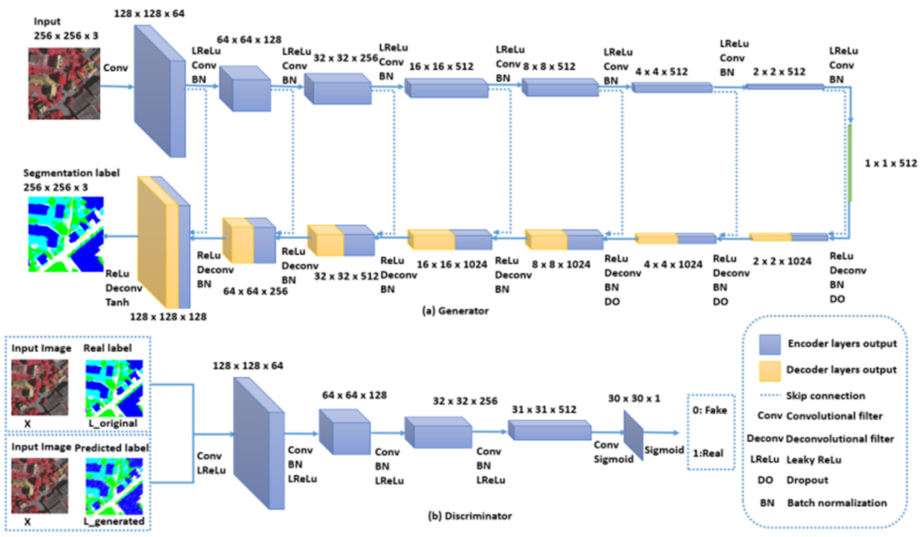
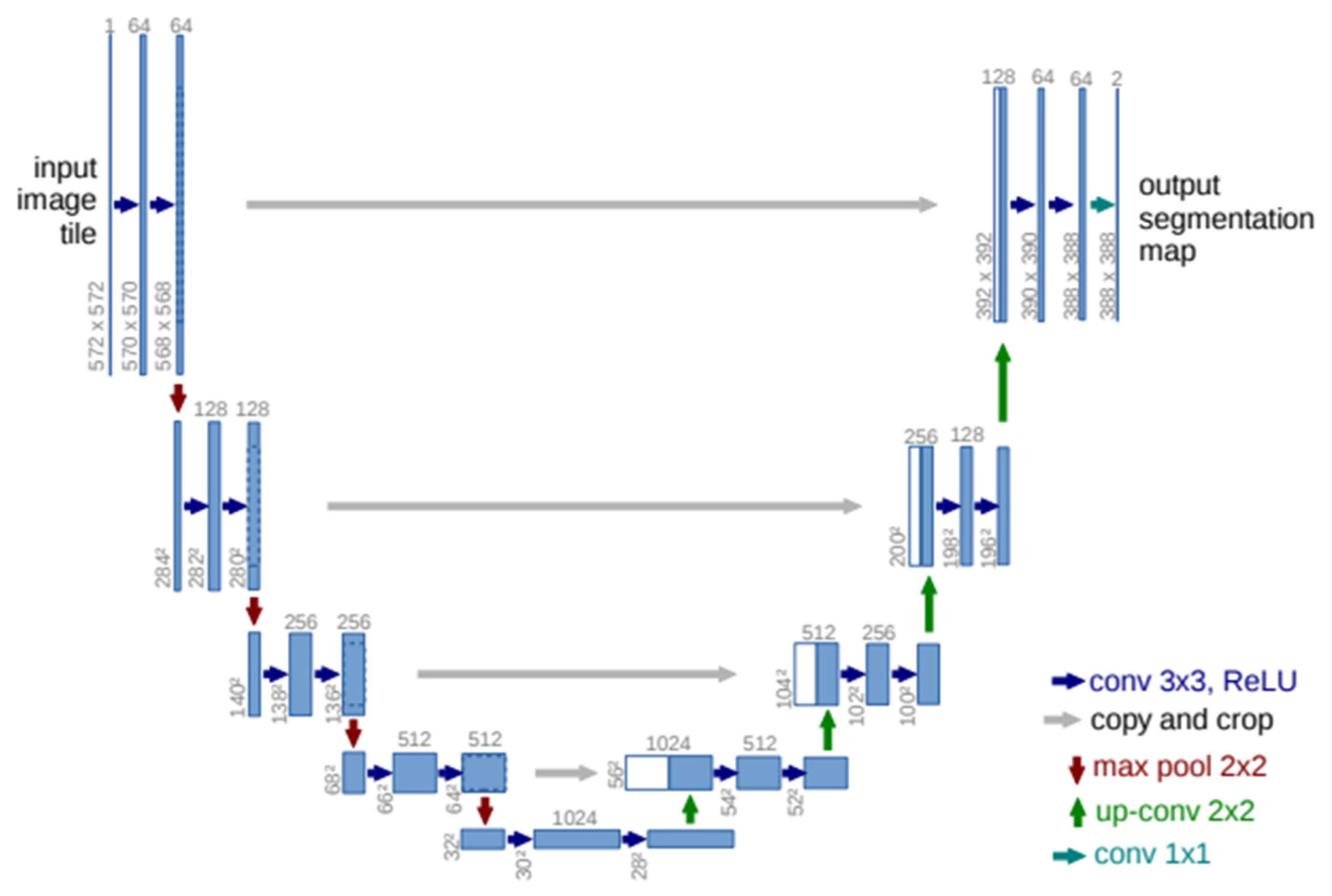
3.2. To Translate Pictures from Pixel to Pixel, a Conditional Generative Adversarial Network Is Utilized

Pixel to Pixel icon conversion [18] is a GAN class that learns a mapping process between an experiential PCA-distorted spectrum picture x and accidental sound vector z and a segmentation facade y, G: (x, z) y, where G is the generator reproduction capable of manufacturing a segmentation mask that cannot distinguish between images before or after “real” imagery is shown by an adversarial-taught discriminator, E. The generator’s bogus segmentation masks have also been trained into Model E [20]. The GANs are depicted schematically in Figure 1. The G model receives just PCA-modified spectral images and attempts to create a segmentation mask. The E model includes both the spectral image after PCA processing and the physically labeled objective segmentation map during the training phase; the G model learns how to synthesize convincing segmentation masks using PCA-converted spectral pictures, whereas the E model learns to detect whether the G model-synthesized segmentation masks are genuine or deceitful [20]. The G model achieves equilibrium after a significant amount of training, allowing it to provide convincing segmentation masks. The goal function of GANs may be inferred from Equation (1):

$$L_{cGAN}\left(G,D\right)=E_{x,y}\left[logD\left(x,y\right)\right]+E_{x,y}\left[log(1-D\left(x,G\left(x,z\right)\right)\right]$$

(1)

where G attempts to limit this goal while an adversary E tries to maximize it as Equation (2); D(x, y) represents the probability that (x, y) comes from the real data

$$G^{*}=arg \underset{G}{min} \underset{D}{max}{L}_{GAN}\left(G,D\right)$$

(2)

In a prior study, combining the GAN’s aim by an additional traditional defeat, such as K1, was found to be effective for achieving a near-ground truth output in the K1 sense for the G model. In comparison to K2, K1 supports less blurring during picture synthesis. Equation (3) can be used to impose the K1 on the G model:

$$L_{L1}\left(G\right)=E_{x,y,z}[y-G\left(x,z{)}_1\right]$$

(3)

The final object Equation (4) is obtained by combining the objectives (2) and (3):

$$G^{*}=arg \underset{G}{min} \underset{D}{max}{L}_{cGAN}\left(G,D\right)+\lambda L_{L1}\left(G\right)$$

(4)

The G model employed a “U-net” architecture in this investigation, as shown in Figure 2, whereas for the E model a convolutional “Pitchman” classifier was utilized. To collect restricted method figures, the Patch GAN classifier was employed. The G replica is taught via adversarial defeat, which forces it to generate accurate segmentation maps [21]. The K1 loss stuck between the estimated segmentation and the physically annotated segmentation map is also used to update the G model. A64-A128-A256-A512-A512-A1024. The E model’s A64-A128-A256-A512 architecture was as follows: A64-A128-A256-A512, where A denotes convolution, and the number denotes the amount of difficulty filters [1]. The difficulty layers of the E model were coupled with LeakyReLU and the concluding coating was fed into a sigmoid start for dual object categorization. Since the goal was a binary classification of true or false, the E model was developed using an adaptive minute optimizer through a knowledge speed of 1/2 0.003 and a loss function of ‘binary_ cross-entropy.’ The last GAN model combines the G and E model, with the E model updated with ‘double cross entropy’ and the G model updated with ‘mean absolute error’. The optimizer was used to generate the final GAN model, which had a knowledge rate of 1/2 0.0003 and a learning rate of 1/2 0.0003. The total number of epochs was 95, with the number of batches in each epoch equivalent to the digit of preparation samples, for a sum of 95 guidance iterations [22]. After training the model, the segmentation masks were built using the single G model. The position fact segmentation mask was used to assess the performance of the segmentation, and junction in excess of amalgamation score were considered using the synthesized segmentation façade. The denoted and normal deviation of IOUs computed on 900 arbitrarily selected picture patches as the test set picture and the reality segmentation mask were used to determine the final IOU score.

3.3. When Compared to the Beginning

The normalized difference vegetation index, a frequently used threshold-based approach, was employed because a baseline contrasts to the p2p GAN replica, which was old. The NDVI method was utilized because the ethereal pictures applied for the expression showed vegetation with a strong contrast after NDVI estimate. A threshold can be set to differentiate the plants from the backdrop when the plant’s contrast with the background is particularly high [23,24]. For the second baseline comparison, a pixel-by-pixel binary partial least-square discriminating analysis was carried out. The whole spectral image’s binary segmentation mask was created pixel-by-pixel using the PLS-EA model, which was calibrated using plant and background spectra collected by hand. It is important to recall that, unlike the GAN model employed in this work, the pixel-wise PLS-EA model ignores the training based on the geographic background of the imagery and is incomplete with respect to the spectra available in sight [23]. The peer-to-peer GAN modeling was performed with Python (3.6).

4. Results and Discussion

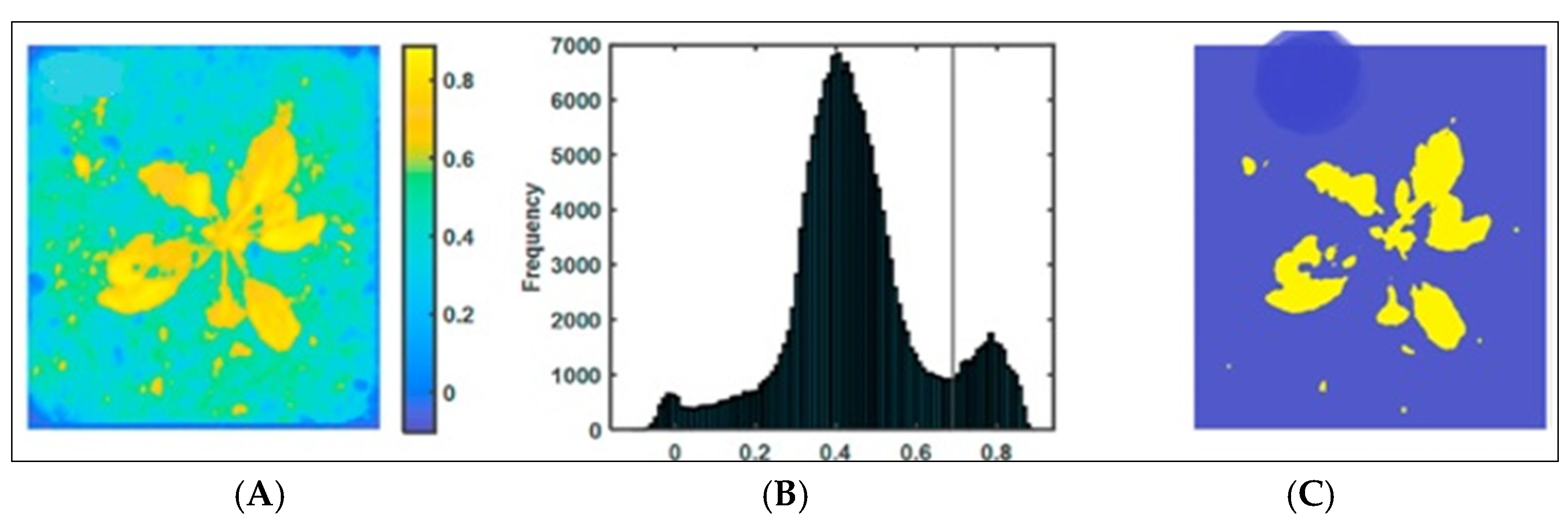
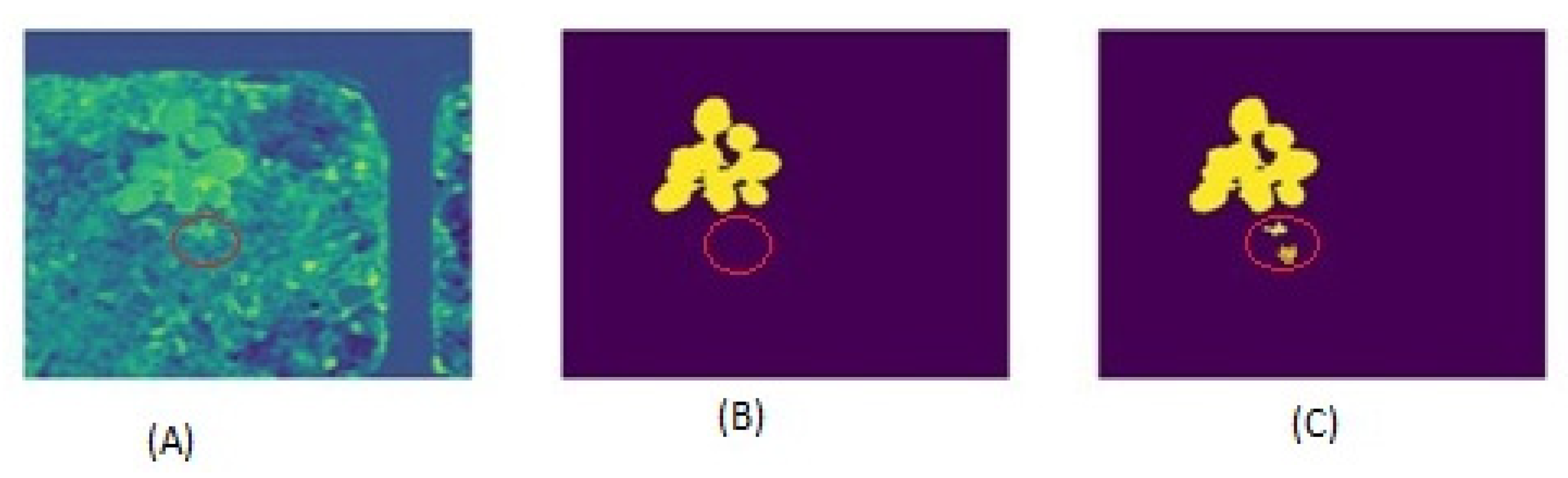
4.1. A Plant Picture with a Dirt Backdrop to Show the Limitations of Threshold-Based Segmentation Analysis with Threshold

Two baseline methodologies were used to compare the p2p GAN-based picture conversion performance. The primary solution employed threshold-based NDVI image segmentation, whereas the second used pixel-shrewd segmentation based on PLS DA methodology. Figure 3 depicts the consequences of the doorsill base segmentation. As an example, Figure 3 shows a sole plant selected as the whole picture series [25]. Figure 3A depicts the calculated NDVI image. The pixels in the NDVI images of the plants have a high intensity, whereas the pixels in the background have a lesser strength. Although certain pixels in the background appear to be brilliant, this might be due to the presence of resources with comparable spectral qualities as foliage. The plants had a higher total NDVI score, which is consistent with the NDVI variety of one to one, with the healthy green plants having principles of one. The NDVI image’s histogram of pixel intensity exhibits distinct peaks, which could be attributed to the image’s plant and environment components (Figure 3B). The peak at 0.8, for example, relates to the stand in Figure 3A as NDVI principles are superior for healthy green plant life, but the peak around 0.4 is associated with the background, which consists of pixels for material with comparable spectral properties to plants. A doorstep of 0.70 was used as part of the image base under two peaks in Figure 3B. Many plant pixels were identified as background pixels, whereas other plant pixels, particularly those associated to the place stalk, were classified as surroundings-pixels [26]. Two problems contributed to the poor performance of threshold-based segmentation. First, there were components with spectral qualities comparable to the plant, making it difficult to select an appropriate doorsill. The subsequent issue was that the threshold-based technique was pixel-based and did not take into account the spatial situation of the picture, such as how a plant looked in layman’s words.

The plants’ denoted spectrum is identical to those by means of a climax at 500 nm with a trough at 700 nm, which corresponds to chlorophyll pigments of healthy green foliage. The changes in the reflectance between 700 and 830 nm have also been linked to photosynthetic action. The change in the reflectance in the region of ≥830 nm has been linked to a moisture-affected leaf arrangement. Then, using PLS analysis on a batch of images, a pixel-based classifier was created, which comprised 3500 random spectra, with 1700/1700 pixels corresponding to plants/background pixels. Figure 4A, presents the spectrum of plant and backdrop, Figure 4B, presents the fake output that was chosen as the best after a comparison of the original image. The real output, and the fake output shows the PLS decomposition explained by the variance plot [27]. The explained variance curve for the classes (red) demonstrates that the explained variable stabilizes at six latent variables (LVs; hence, the final PLS model was built using six LVs. Figure 3C shows the weakening vector for the six LVs’ PLS representations. The visible and red-edged parts of the regression vector were given higher weights, which might be connected to pigments found in plant life except not in the background. In addition, the score for the initial two main mechanism of the PLS representation are given in Figure 4D, which had many backdrops, and where the pixels scored similarly to the plants, implying that the environment contains pixels with comparable spectral qualities to the vegetation [24]. Some of the plant and environmental pixels were misclassified, as seen in the confusion matrix. Furthermore, the percentage of pixels misclassified as plant backgrounds was greater than the percentage of pixels misclassified as plant background. In general, categorization is important. An example of segmentation using PLS-DA model is presented in the Figure 5. Which is representing the NDVI picture, ground truth mask and PLS DA based segmentation. In addition, Figure 6 represents the loss obtained during the generator phase and the discriminator phase.

In Figure 7, the loss for the discriminator and generator models evolved. Only 0.9% of pixels were misclassified, resulting in a 99.1% accuracy rate. To acquire a chart picture of the presentation of the PLS-DA technique, it was evaluated by applying the model to a sovereign test picture and estimating the segmentation facade. The segmented test picture of a plant, shown in Figure 7, was an excellent example. To obtain a comparable arithmetic calculation for the segmentation presentation of the PLS-DA-based pixel categorization, the intersection over union (IoU) scores from the independent test set for the 900 sub-samples photos (512 512) were generated. The PLS-DA-based classification has an IoU score of 0.82 0.15. Since the presentation of the p2p GAN-based image segmentation was to be evaluated using the same set of 1000 sample photos, the IoU achievement for the PLS-DA method may be a good comparison to the IoU achieved for the p2p GAN in the next section.

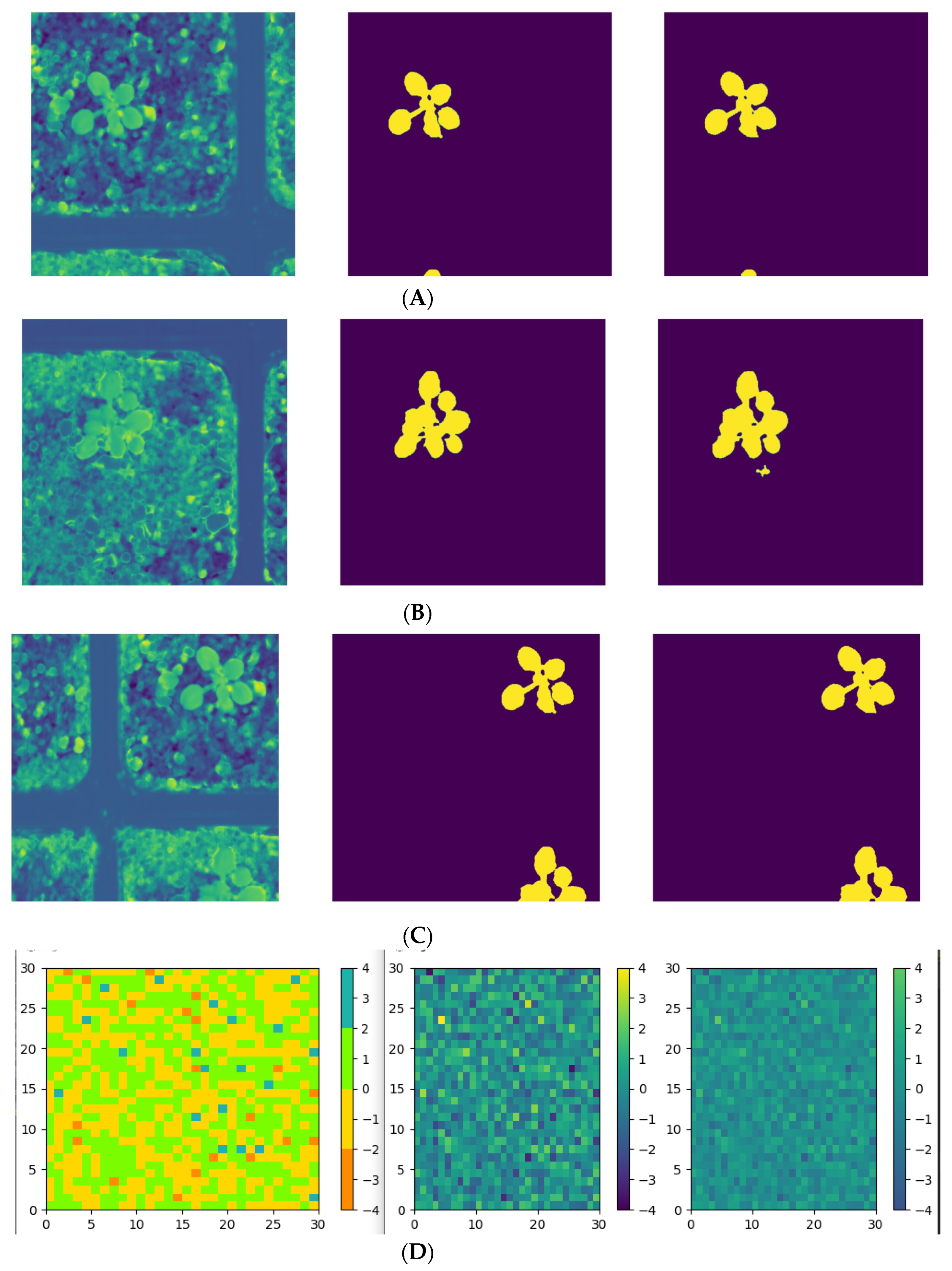
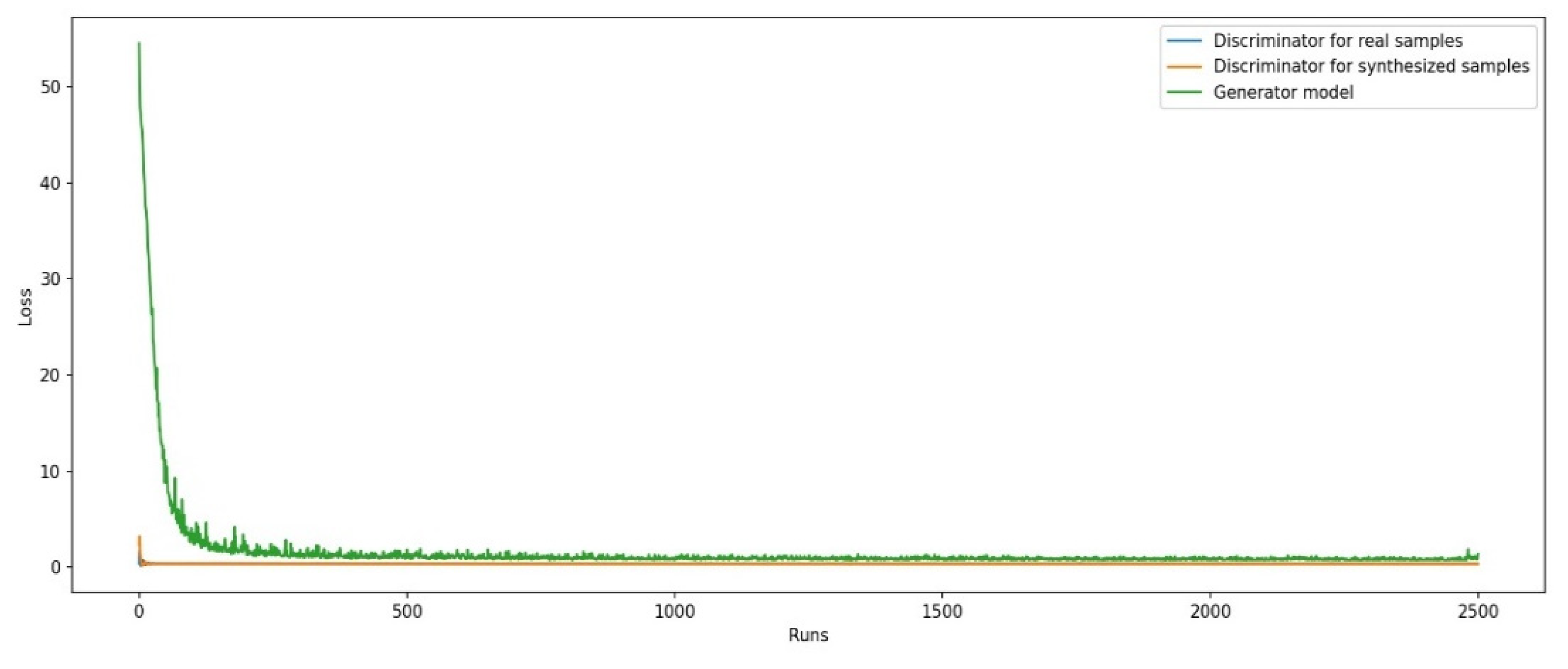
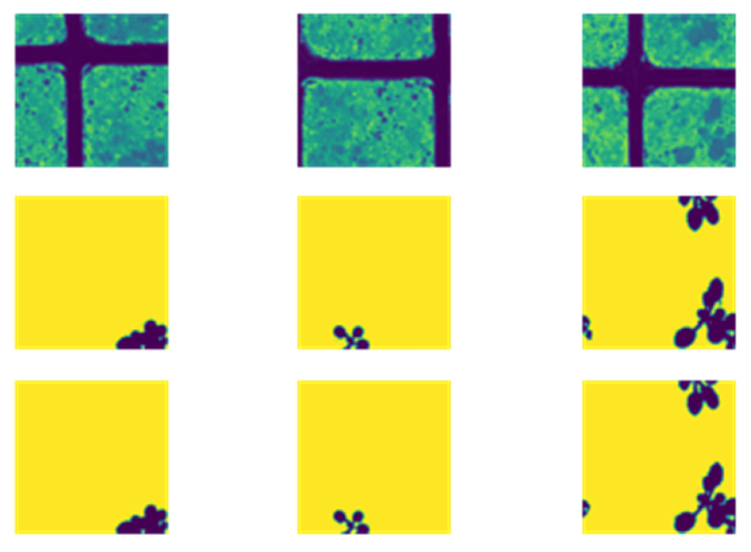
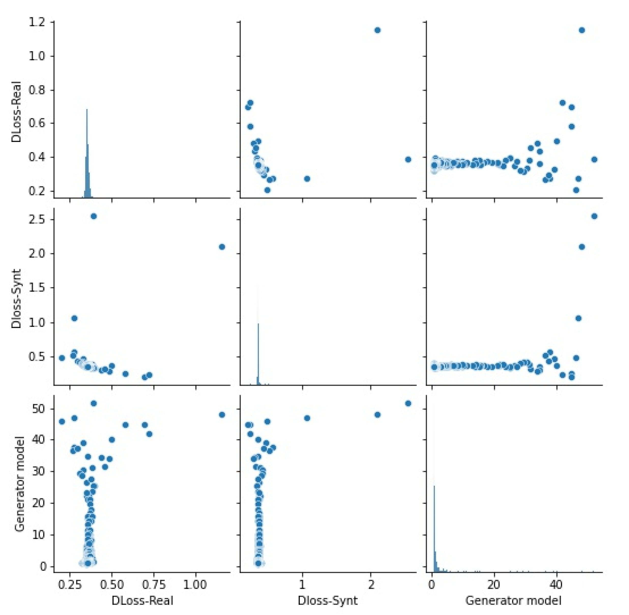
4.2. Image Segmentation from Pixels to Pixels Using Provisional Generative Adversarial Networks

Figure 7 shows the p2p GAN model’s training performance for segmenting plants from the backdrop. The p2p GAN was used to train both the discriminator and generator models, which learned to synthesis segmentation masks during training and to assess whether the resulting similes are genuine or fraudulent [28]. The discriminator representation, in comparison to the generator model, achieved a low loss after a few early runs; however, the producer model’s rate of defeat was at first large but then decreased as it increasingly learned to synthesize the segmentation masks. The discriminator and generator models ultimately reached equilibrium after 32,000 iterations, and the generator model showed no further progress. As a result, the segmentation facade for the self-governing examination set of pictures was created using the final generator model. Figure 8 shows four exemplary picture subsamples of the independent investigation set image. The position-fact segmentation mask and the p2p GAN outputs were fairly similar [29]. In comparison to the presentation of the pixel-based PLS-DA categorization, the IoU that was achieved measured on the 900 sub sample photographs as of the sovereign test images was 0.98 ± 0.06.

5. Conclusions

In this paper, we presented an image translation pixel-to-pixel (p2p) method segmenting spectral images using a generative adversary network (GAN). This is the first study to demonstrate an artificial completion of pixel-to-pixel provisional generative adversarial networks for the dispensation of phantom images using a geographical background and spectral data. As contextual information is rarely used in chemometrics through phantom image processing, the matrices are normally processed pixel-by-pixel after the pixel-wise processing, molded into visuals, and shown as spatial maps. The disadvantage of converting photos into matrices and dispensing information pixel by pixel is that it ignores the spatial context of spectral images. In our approach, a unique use of spectral images for translation to a segmentation map was reported. The results demonstrated the superior technique of the p2p GAN outperformed the pixel-wise data processing alternatives in interpreting spectral imagery utilizing both geographical context and spectral information. When the backdrop comprises materials with comparable spectral characteristics, then the two pixel-based techniques—doorsill-based and pixel-based categorization segmentation approaches—suffered, as seen in the presented scenario of plant segmentation. The existence of unrelated pixels with equal spectral qualities had no effect on the p2p GAN approach, which combines both spatial context and spectral information. As a result, deep learning-based advanced image-processing algorithms offer numerous possibilities for enhancing spectral image dispensation, especially when both spatial contexts and spectral data are used.

References

1. Coic, L.; Sacré, P.-Y.; Dispas, A.; De Bleye, C.; Fillet, M.; Ruckebusch, C.; Hubert, P.; Ziemons, E. Pixel-based Raman hyperspectral identification of complex pharmaceutical formulations. Anal. Chim. Acta 2021, 1155, 338361. [Google Scholar] [CrossRef] [PubMed]
2. Shan, J.; Zhao, J.; Zhang, Y.; Liu, L.; Wu, F.; Wang, X. Simple and rapid detection of microplastics in seawater using hyperspectral imaging technology. Anal. Chim. Acta 2019, 1050, 161–168. [Google Scholar] [CrossRef]
3. Adao, T.; Hruška, J.; Pádua, L.; Bessa, J.; Peres, E.; Morais, R.; Sousa, J.J. Hyperspectral imaging: A review on UAV-based sensors, data processing and applications for agriculture and forestry. Remote Sens. 2017, 9, 1110. [Google Scholar] [CrossRef] [Green Version]
4. Arendse, E.; Fawole, O.A.; Magwaza, L.S.; Opara, U.L. Non-destructive prediction of internal and external quality attributes of fruit with thick rind: A review. J. Food Eng. 2018, 217, 11–23. [Google Scholar] [CrossRef]
5. Botelho, B.G.; Oliveira, L.S.; Franca, A.S. Fluorescence spectroscopy as tool for the geographical discrimination of coffees produced in different regions of Minas Gerais State in Brazil. Food Control. 2017, 77, 25–31. [Google Scholar] [CrossRef]
6. Mishra, P.; Schmuck, M.; Roth, S.; Nicol, A.; Nordon, A. Homogenising and segmenting hyperspectral images of plants and testing chemicals in a high-throughput plant phenotyping setup. In Proceedings of the 2019 10th Workshop on Hyperspectral Imaging and Signal Processing: Evolution in Remote Sensing (WHISPERS), Amsterdam, The Netherlands, 24–26 September 2019; IEEE: New York, NY, USA; pp. 1–5. [Google Scholar]
7. Asaari, M.S.M.; Mishra, P.; Mertens, S.; Dhondt, S.; Inzé, D.; Wuyts, N.; Scheunders, P. Close-range hyperspectral image analysis for the early detection of stress responses in individual plants in a high-throughput phenotyping platform. ISPRS J. Photogramm. Remote Sens. 2018, 138, 121–138. [Google Scholar] [CrossRef]
8. Fahlgren, N.; Gehan, M.A.; Baxter, I. Lights, camera, action: High-throughput plant phenotyping is ready for a close-up. Curr. Opin. Plant Biol. 2015, 24, 93–99. [Google Scholar] [CrossRef] [Green Version]
9. Mishra, P.; Polder, G.; Gowen, A.; Rutledge, D.N.; Roger, J.-M. Utilising variable sorting for normalisation to correct illumination effects in close-range spectral images of potato plants. Biosyst. Eng. 2020, 197, 318–323. [Google Scholar] [CrossRef]
10. Mishra, P.; Karami, A.; Nordon, A.; Rutledge, D.N.; Roger, J.-M. Automatic de-noising of close-range hyperspectral images with a wavelength-specific shearlet-based image noise reduction method. Sens. Actuators B Chem. 2019, 281, 1034–1044. [Google Scholar] [CrossRef]
11. Kandpal, L.M.; Tewari, J.; Gopinathan, N.; Boulas, P.; Cho, B.K. In-process control assay of pharmaceutical microtablets using hyperspectral imaging coupled with multivariate analysis. Anal. Chem. 2016, 88, 11055–11061. [Google Scholar] [CrossRef]
12. Ferreira, K.B.; Oliveira, A.G.G.; Gonçalves, A.S.; Gomes, J.A. Evaluation of hyperspectral imaging visible/near infrared spectroscopy as a forensic tool for automotive paint distinction. Forensic Chem. 2017, 5, 46–52. [Google Scholar] [CrossRef]
13. Chen, G.; Qian, S.E. Denoising of hyperspectral imagery using principal component analysis and wavelet shrinkage. IEEE Trans. Geosci. Remote Sens. 2010, 49, 973–980. [Google Scholar] [CrossRef]
14. Wahabzada, M.; Mahlein, A.K.; Bauckhage, C.; Steiner, U.; Oerke, E.C.; Kersting, K. Plant phenotyping using probabilistic topic models: Uncovering the hyperspectral language of plants. Sci. Rep. 2016, 6, 22482. [Google Scholar] [CrossRef] [PubMed] [Green Version]
15. Heylen, R.; Burazerovic, D.; Scheunders, P. Fully constrained least squares spectral unmixing by simplex projection. IEEE Trans. Geosci. Remote Sens. 2011, 49, 4112–4122. [Google Scholar] [CrossRef]
16. De Beer, T.; Bodson, C.; Dejaegher, B.; Walczak, B.; Vercruysse, P.; Burggraeve, A.; Lemos, A.; Delattre, L.; Heyden, Y.V.; Remon, J.; et al. Raman spectroscopy as a process analytical technology (PAT) tool for the in-line monitoring and understanding of a powder blending process. J. Pharm. Biomed. Anal. 2008, 48, 772–779. [Google Scholar] [CrossRef] [PubMed]
17. Sacré, P.-Y.; Lebrun, P.; Chavez, P.-F.; De Bleye, C.; Netchacovitch, L.; Rozet, E.; Klinkenberg, R.; Streel, B.; Hubert, P.; Ziemons, E. A new criterion to assess distributional homogeneity in hyperspectral images of solid pharmaceutical dosage forms. Anal. Chim. Acta 2014, 818, 7–14. [Google Scholar] [CrossRef] [PubMed] [Green Version]
18. Cailletaud, J.; Bleye, C.; Dumont, E.; Sacré, P.Y.; Gut, Y.; Bultel, L.; Ginot, Y.M.; Hubert, P.; Ziemons, E. Towards a spray-coating method for the detection of low-dose compounds in pharmaceutical tablets using surface-enhanced Raman chemical imaging (SER-CI). Talanta 2018, 188, 584–592. [Google Scholar] [CrossRef]
19. El-Hagrasy, A.S.; Delgado-Lopez, M.; Drennen, J.K., III. A process analytical technology approach to near-infrared process control of pharmaceutical powder blending: Part II: Qualitative near-infrared models for prediction of blend homogeneity. J. Pharm. Sci. 2006, 95, 407–421. [Google Scholar] [CrossRef]
20. Alexandrino, G.L.; Poppi, R. NIR imaging spectroscopy for quantification of constituents in polymers thin films loaded with paracetamol. Anal. Chim. Acta 2013, 765, 37–44. [Google Scholar] [CrossRef]
21. Kamruzzaman, M.; ElMasry, G.; Sun, D.-W.; Allen, P. Prediction of some quality attributes of lamb meat using near-infrared hyperspectral imaging and multivariate analysis. Anal. Chim. Acta 2012, 714, 57–67. [Google Scholar] [CrossRef]
22. Duponchel, L. Exploring hyperspectral imaging data sets with topological data analysis. Anal. Chim. Acta 2018, 1000, 123–131. [Google Scholar] [CrossRef] [PubMed]
23. Xu, X.; Li, J.; Wu, C.; Plaza, A. Regional clustering-based spatial preprocessing for hyperspectral unmixing. Remote Sens. Environ. 2018, 204, 333–346. [Google Scholar] [CrossRef]
24. Fauteux-Lefebvre, C.; Lavoie, F.; Gosselin, R. A Hierarchical Multivariate Curve Resolution Methodology to Identify and Map Compounds in Spectral Images. Anal. Chem. 2018, 90, 13118–13125. [Google Scholar] [CrossRef] [PubMed]
25. Bøtker, J.; Wu, J.X.; Rantanen, J. Hyperspectral imaging as a part of pharmaceutical product design. In Data Handling in Science and Technology; Elsevier: Amsterdam, The Netherlands, 2020; Volume 32, pp. 567–581. [Google Scholar]
26. Biancolillo, A.; Boqué, R.; Cocchi, M.; Marini, F. Data fusion strategies in food analysis. In Data Handling in Science and Technology; Elsevier: Amsterdam, The Netherlands, 2020; Volume 31, pp. 271–310. [Google Scholar]
27. Mitsutake, H.; Castro, S.R.; de Paula, E.; Poppi, R.J.; Rutledge, D.N.; Breitkreitz, M.C. Comparison of different chemometric methods to extract chemical and physical information from Raman images of homogeneous and heterogeneous semi-solid pharmaceutical formulations. Int. J. Pharm. 2018, 552, 119–129. [Google Scholar] [CrossRef]
28. de Juan, A. Multivariate curve resolution for hyperspectral image analysis. In Data Handling in Science and Technology; Elsevier: Amsterdam, The Netherlands, 2020; Volume 32, pp. 115–150. [Google Scholar]
29. Xu, K.; Zhao, Y.; Zhang, L.; Gao, C.; Huang, H. Spectral–Spatial Residual Graph Attention Network for Hyperspectral Image Classification. IEEE Geosci. Remote Sens. Lett 2021, 19, 5509305. [Google Scholar] [CrossRef]
Figure 1. To convert PCA-converted spectral pictures to segmentation maps [2].
Electronics 11 02611 g001
Figure 2. UNET architecture used in the GAN model [22].
Electronics 11 02611 g002
Figure 3. The limitations of threshold-based segmentation. (A) Normalized differences are those that have been rounded to the nearest tenth of a percentile and an illustration of the plants index, (B) Histogram of NDVI pixel intensities, and (C) Segmentation based on thresholds [1].
Electronics 11 02611 g003
Figure 4. A digest of the pixels based PLS DA segmentation method. (A) Denotes spectrum of plants and the backdrop; (B)The fake output was chosen as the best after a comparison of the original image, the real output, and the fake output; (C) Categorization of the truth vector of the NDVI opinion and PLS-DA analysis, performed using Python pilchard; and (D) PLS scores for the first and second pictures’ major components, as well as the matrix and sounding region.
Electronics 11 02611 g004
Figure 5. An example of segmentation using the PLS-DA model’s pixel-based application. (A) The NDVI picture, (B) ground-truth mask and (C) PLS DA predict segmentation facade, respectively. The scarlet loop in the shape represents the area anywhere the PLS-DA base segmentation miss classified pixels. (Explanation of the color reference in this shape fable, please see the mesh account of this editorial).
Electronics 11 02611 g005
Figure 6. During the pixel2pixel condition generative adversarial network training.
Electronics 11 02611 g006
Figure 7. This pair plot represents relationship between output variables extracted from our model. Variables compared here are Discriminator loss for synthesized samples (fake images), Discriminator loss for real samples (Real images), and generator loss.
Electronics 11 02611 g007
Figure 8. The spectral image segmentation performance of the pixel-to-pixel conditional generative adversarial network. The first column shows fake color spectrum photos, the second column shows masks for segmentation based on ground truth, and the third column shows pixel2pixel GAN segmentation, from left to right. Three sequential outputs are compared to the real image, the predicted output, and the false image created.
Electronics 11 02611 g008
Publisher’s Note: MDPI stays neutral with regard to jurisdictional claims in published maps and institutional affiliations.