Abstract
In the last two decades, Radio Frequency Identification (RFID) technology has attained prominent performance improvement and has been recognized as one of the key enablers of the Internet of Things (IoT) concepts. In parallel, extensive employment of Machine Learning (ML) algorithms in diverse IoT areas has led to numerous advantages that increase successful utilization in different scenarios. The work presented in this paper provides a use-case feasibility analysis of the implementation of ML algorithms for the estimation of ALOHA-based frame size in the RIFD Gen2 system. Findings presented in this research indicate that the examined ML algorithms can be deployed on modern state-of-the-art resource-constrained microcontrollers enhancing system throughput. In addition, such utilization can cope with latency since the execution time is sufficient to meet protocol needs.
1. Introduction
The Internet of Things (IoT) has become a pervasive environment in which smart objects interact and exchange information by sensing the ambiance of their surroundings. One of the major technologies that enable IoT is Radio Frequency Identification (RFID), which can utilize Wireless Information and Power Transfer (WIPT) in its applications that include access control, parking management, logistics, retail, etc. [1]. In large-scale infrastructures, such as commercial warehouses, reading RFID tags, such as ultra-high-frequency ones, comes at a high cost and can involve a large volume of data [2]. In general, RFID presents radio technology that acts as a communication medium between a reader and the tag, with a unique identifier used for communication [3]. In general, the RFID tag is distinguished by the presence or absence of the battery [4]. Passive tags are self-powered and communicate using the same RF waves emitted by the reader antennas, known as backscattering technology [5]. Among the existing technologies, passive Gen2 technology is considered the most attractive in IoT applications due to its simple design, flexibility, cost and performance [6,7]. Gen2 as a standard is used on the physical and MAC levels to establish reliable communication between the reader and a tag. Readers must provide sufficient power to energize tags and respond to the necessary information since they are not equipped with batteries. The energy levels that tags can extract are quite low and, therefore, cannot afford energy-efficient MAC schemes [8]. In general, the MAC of RFID is random, and there are two widely used methods to achieve it: the first is a binary tree, and the second is the ALOHA-based protocol [4]. In the binary tree protocol, continuous YES/NO communication is achieved between a reader and tags, while with the ALOHA protocol tag initiates communication with a request from the reader [9,10,11].
One of the commonly utilized ALOHA-based protocols is the Dynamic Framed Slotted ALOHA (DFSA) since it has the most prominent performance, which is the highest throughput. DFSA belongs to a group of time division multiple access (TDMA) protocols, where communication between a reader and tags is divided into time frames, which are, in turn, divided into time slots [12]. The beginning of the interrogation process in DFSA is induced by the reader’s announcement of the frame size [6]. This is performed by the reader sending a QUERY command and the value of the main protocol parameter Q for the tags [13]. The value of Q is an integer ranging from 0 to 15 that sets the frame size at . From there on, all tags that are being interrogated will occupy a randomly selected position in the frame (commonly known as a slot) and will onward reply back to the reader when their slot is being interrogated. Based on such an access control scheme, three diverse scenarios may happen: (a) only one tag is in the slot (the successful slot), (b) no tags in the slot (empty slot) and (c) numerous tags have taken the same spot (collision) [6]. The overall number of successful, empty and collision slots is denoted with S, E and C, respectively. An example of an interrogating frame is exhibited in Figure 1.
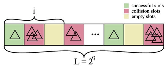
Figure 1.
An example of an interrogating frame of frame size . i represents the size of a particular part of the frame.
Therefore, the frame size is equal to the sum of successful, empty and collision slots, i.e., . According to the previous notation, the throughput is defined using Equation (1) as:
therefore, the main goal in DFSA systems is to increase the number of successful slots S within the frame size L. As tags are fitting their slots randomly, previous studies [14] show that the maximum throughput will reach its maximum value of approximately 37% when the size of the frame equals the number of tags. In usual situations, the number of tags is unknown and has to be estimated in order to set an adequate frame size and, consequently, achieve maximum throughput.
Aiming to improve the throughput of RFID systems, the research presented in this paper utilizes Machine Learning classifiers as an approach for efficient tag number estimation. The performance of the ML algorithms is compared with state-of-the-art solutions, specifically the Improved Linearized Combinatorial model (ILCM) for tag estimation (elaborated in [8]). The study presented in this paper shows that ML classifiers, which use the maximum of the available information gathered from Monte Carlo simulations, can be implemented in standard, mobile RFID readers. What is more, they outperform the state-of-the-art model achieving better throughput. The advances result in achieving optimal performance in tag identification by the reasonable processing time and energy requirements. The paper is structured as follows: Section 2 gives an insight into some commonly applied methods for tag number estimation and provides more detail on the ILCM model. Section 3.1 gives details on the experimental setup and elaboration on the Machine Learning models and the ILCM model used on a particular set of data, continuing with model performance analyses and comparison. Section 5 examines the feasibility and mandatory means for the efficient deployment of ML models on microcontrollers. Overall, an articulate conclusion that emphasizes the obtained results is provided in Section 6.
2. Related Works
Over the past few years, various methods and approaches have been employed for tag estimation. In [15], Vogt presented a method based on Minimum Squared Error (MSE) estimation by minimizing the Euclidean norm of the vector difference between the actual frame statistics and their expected values. The number of empty, successful and collision slots is taken into account. However, the predicted values are calculated under the assumption that the tags in each slot have independent binomial distributions, which leads to unreliable findings. In the research presented by Chen in [14], the authors apply probabilistic modeling of the tag distribution within the frame, which they consider to be a multinomial distribution. By doing so, they obtain the tag number estimation. For each slot, binomial distributions provide occupancy information. However, it does not consider the fact that the number of tags in the interrogation area is limited [16]. An improvement of the previous model was given by research in [17], although this improvement tends to have a high computational cost of implementation for genuine RFID systems [16]. Furthermore, a study presented in [18] offered a unique tag number estimation scheme termed ‘Scalable Minimum Mean Square Error’ (sMMSE), which enhanced accuracy and reduced estimation time. The efficient modification of the frame size is derived from two principal parameters: the first one puts a limit on the slot occupancy, whereupon frame size needs to be expanded, and the second determines the frame size expansion factor. In the research presented in [19], the authors provided an in-depth analysis of some of the most relevant anti-collision algorithms, taking into account the limitations imposed by EPCglobal Class-1 Gen-2 for passive RFID systems. The study classified and compared some of the most important algorithms and optimal frame-length selection. Based on their research results, the authors point out that the maximum-likelihood algorithms achieve the best performance in terms of mean identification delay. Finally, the researchers concluded that the algorithm performance also depends on the computation time for estimating the number of tags.
A study presented in [20] introduced a new MFML-DFSA anti-collision protocol. In order to increase the accuracy of the estimate, it uses a maximum-likelihood estimator that makes use of statistical data from many frames (multiframe estimation). The algorithm chooses the ideal frame length for the following reading frame based on the anticipated number of tags, taking into account the limitations of the EPCglobal Class-1 Gen-2 standard. The MFML-DFSA algorithm outperforms earlier suggestions in terms of average identification time and computing cost (which is lower), making it appropriate for use in commercial RFID readers. The rather novel research given in [21] proposes an RFID tag anti-collision method that applies adjustable frame length modification. The original tag number is estimated based on the initial assumption that the number of tags identified in the first frame is known. The authors present a non-linear transcendental equation-based DFSA (NTEBD) algorithm and compare it to the ALOHA algorithm demonstrating the error rate for experimental results to be less than 5% and improved tag identification throughput by 50%. The authors of [22] present an extension for an anti-collision estimator based on a binomial distribution. They have constructed a simulation module to examine estimator performance in diverse scenarios and have shown that the proposed extension has enhanced performance in comparison to other estimators, no matter if the number of tags is 1000 or 10,000.
As can be observed, the previously mentioned algorithms tend to have high computational costs since they are commonly funded by calculating probabilities. This might present an issue for standard microprocessors that are not adjusted to perform computations of factorials that produce large numbers. To solve the issue, a diverse method for tag estimation has been introduced by researchers in [8], namely the Improved Linearized Combinatorial model. Their approach bypasses the conditional probability calculations by doing them in advance. Further, the estimation model is uncomplicated and provides an effective tag estimation based on linear interpolation given by Equation (2):
where coefficients k and l are derived from Equations (3) and (4), respectively:
In the event of no collision, the formula gives , whereas for cases when , k must be set to 0. Following the tag estimation, the Q value is calculated using Equation (5) as
The results obtained by the authors have indicated that the ILCM shows comparable behavior to state-of-the-art algorithms regarding the identification delay (slots) but is not computationally complex. An extension of their study was performed in [23] by presenting a C-MAP anti-collision algorithm for an RFID system that has lower memory demands.
3. Materials and Methods
3.1. Machine Learning Classifiers for Tag Estimation
The IoT surroundings rich with sensor devices that are interconnected have also yielded the demand for the more efficient monitoring of sensor activities and events [24]. To support diverse IoT use-case scenarios, Machine Learning has emerged as an essential area of scientific study and employment to enable computers to automatically progress through experience [25]. Commonly, ML incorporates data analyses and processing followed by training phases to produce “a model”, which is onward tested. The overall goal is to expedite the system to act based on the results and inputs given within the training phase [26]. For the system to successfully achieve the learning process, distinctive algorithms and models along with data analyses are employed to extract and gain insight into data correlation [27]. Thus far, Machine Learning has been fruitfully applied to various problems such as regression, classification and density estimation [28]. Specific algorithms are universally split into disjoint groups known as Unsupervised, Supervised, Semi-supervised and Reinforcement algorithms. The selection of the most appropriate ML algorithm for a specific purpose is performed based on its speed and computational complexity [27].
Machine Learning applications range from prediction, image processing, speech recognition, computer vision, semantic analysis, natural language processing, as well as information retrieval [29]. In a problem like the estimation of the tag number based on the provided input, one must consider the most applicable classifiers that can deal with a particular set of data. Currently, classification algorithms have been applied for financial analyses, bio-informatics, face detection, handwriting recognition, image classification, text classification, spam filtering, etc. [30]. In a classification problem, a targeted label is generally a bounded number of discrete categories, such as in the case of estimating the number of tags. State-of-the-art algorithms for classification incorporate Decision Tree (DT), k-Nearest Neighbour (k-NN), Support Vector Machine (SVM), Random Forest (RF) and Bayesian Network [31]. In the last decade, Deep Learning (DL) has manifested itself as a novel ML technique that has efficiently solved problems that have not been overcome by more traditional ML algorithms [26]. Considered to be one of the most notable technologies of the decade, DL utilizations have obtained remarkable accuracy in various fields such as image and audio-related domains [26,32]. DL has the remarkable ability to discover the complex configuration of large datasets using a backpropagation algorithm indicating in what manner the machine’s internal parameters need to be altered to calculate and determine each layer’s representation based on the representation of previous layers [33]. The essential principle of DL has been displayed throughout growing research performed in Neural Networks or Artificial Neural Networks (ANN). This approach allows for a layered structure of concepts with multiple levels of abstraction, in which every layer of concepts is made from some simpler layers [26]. Deep Learning has made improvements in problem-solving with regards to discovering intricate configurations of large-sized data and thus has been applied in various domains ranging from image recognition, speech recognition, natural language understanding, sentiment analysis and many more [33]. Machine Learning classifier performance has been extensively analyzed in the last decade [34,35,36,37], providing a systematical insight into the classifiers’ key attributes. Table 1 provides a comparison of the advantages and limitations of commonly utilized ML classifiers.

Table 1.
The advantages and limitations of commonly utilized ML classifiers [34,35,36,37].
Tag number estimation can be regarded as a multi-class classification problem. Amongst many classifiers, Random Forest has been considered a simple yet powerful algorithm for classification, successfully applied in numerous problems such as image annotation, text classification, medical data etc. [38]. RF has been proven to be very accurate when dealing with large datasets; it is robust to noise and has a parallel architecture that makes it faster than other state-of-the-art classifiers [39]. Furthermore, it is also very efficient in stabilizing classification errors when dealing with unbalanced datasets [40]. On the other hand, Neural Networks offer great potential for multi-class classification due to their non-linear architecture and prominent approximation proficiency to comprehend tangled input–output relationships between data [41].
Discriminative models, such as Neural Networks and Random Forest, can model the decision boundary between the classes [42], thus providing vigorous solutions for non-linear discrimination in high-dimensional spaces [43]. Therefore, their utilization for classification proposes has proven to be successful and efficient [44]. Both algorithms are able to model linear as well as complex non-linear relationships. However, Neural Networks have a greater potential here due to their construction [45]. On the other hand, RF outperforms NN in arbitrary domains, particularly in cases when the underlying data sizes are small, and no domain-specific insight has been used to arrange the architecture of the underlying NN [21]. Although NN is an expressively rich tool for complex data modeling, they are prone to overfitting on small datasets [46] and are very time-consuming and computationally intensive [45]. Furthermore, their performance is frequently sensitive to the specific architectures used to arrange the computational units [21] in contrast to the computational cost and time of training a Random Forest, requiring much less input preparation [45]. Finally, although RF needs less hyper-parameter tuning than NN, the acquisitive feature space separation by orthogonal hyper-planes produces typical stair or box-like decision surfaces, which can be beneficial for some datasets but sub-optimal for others [46].
Following the stated reasoning, Neural Network and Random Forest have been applied in this research for tag number estimation based on the scenarios that occur during slot interrogation.
3.1.1. Experimental Setup
To obtain valuable data for model comparison, Monte Carlo simulations were performed to produce an adequate number of possible scenarios that may happen during the interrogation procedure in DFSA. Detailed elaboration of the mathematical background of the Monte Carlo method that has been applied for this research has been elaborated in research prior to this one and presented in [11]. The selected approach for Monte Carlo simulations of the distribution of tags in the slots follows the research performed in studies [8] and [23]. Simulations were executed for frame sizes and 256, i.e., for and 8, where the number of tags was in the range of (this range was chosen based upon experimental findings elaborated in [23]). For each of the frame sizes and the number of tags, random 100,000 distributions of E empty slots, successful slots S and collision slots C were realized and are presented in Table 2.
Table 2.
Snapshot of the obtained data.
Data obtained from the simulations were given to Neural Network, Random Forest and the ILCM models for adequate performance comparison and analyses of the accuracy of tag estimation.
All of the models and simulations were performed on a dedicated computer for such tasks. To be precise, the machine has an Intel(R) Core(TM) i7-7700HQ@2.80 GHz processor, 16 GB of RAM and NVIDIA GeForce GTX 1050 Ti with 768 existing cores running on a 64-bit Windows 10 operating system. Furthermore, to realize more efficient computing with the GPU, the Deep Neural Network NVIDIA CUDA library (cuDNN) [47] was applied. The Keras 2.3.1. Python library was employed, which operates on top of a source built upon Tensorflow 2.2.0 with CUDA support for different batch sizes.
3.1.2. Neural Network Model
In general, a Neural Network is made out of an artificial neuron and layer: the input, the hidden layer (or layers) and the output layer are all interconnected [26], as exhibited in Figure 2.
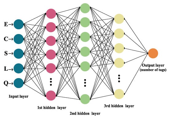
Figure 2.
Architecture of the Neural Network model.
Aiming to imitate the behavior of real biological neurons, the course of learning within a NN unfolds through uncovering hidden correlations amongst the sequences of input data throughout layers of neurons. The outputs from neurons in one layer are onward given as inputs to the neurons in the next layer. A formal mathematical definition of an artificial neuron given by Equation (6) is as follows.
Definition 1.
An artificial neuron is the output of the non-linear mapping θ applied to a weighted sum of input values x and a bias β defined as:
where represents the matrix of weights and is called an artificial neuron.
The weights are appointed considering the inputs’ correlative significance to the other inputs, and the bias ensures a consistent value is added to the mapping to ensure successful learning [48]. Generally, the mapping is known as the activation (or transfer) function. Its purpose is to keep the amplitude of the output of the neuron in an adequate range of or [49]. Although activation functions may be linear and non-linear, usually the non-linear ones are more frequently utilized. The most recognizable ones are ordinary Sigmoids or the Softmax function, such as the hyperbolic tangent , in contrast to Rectified Linear Unit (ReLU) function: [33]. The selection of a particular activation function is based on the core problem to be solved by applying the Neural Network [50].
The architecture of the NN model displayed in this research is constructed of five layers, as depicted in Figure 2. The first one is the input layer, followed by three hidden layers (one Dropout layer), and the final is the output layer. Applied activation functions were ReLU (in hidden layers) and Softmax (within the output layer). Data used for the input layer were number Q, frame size L and the number of S successful, E empty and C collision slots. The number of tags that are associated with a particular distribution of slots within a frame is classified in the final exit layer.
The data were further partitioned in a ratio, with of the data used for training and the other for testing, with the target values being the number of tags, and all other values were provided as input. The training data were pre-processed and normalized, whereas target values were coded with One Hot Encoded with Keras library for better efficiency. By doing so, the integer values of the number of tags are encoded as binary vectors. The dropout rate (probability of setting outputs from the hidden layer to zero) was specified to be 20%. The number of neurons varies based on the frame size, ranging from 64 to 1024 for the first four layers.
Since the classification of the number of tags is a multi-class classification problem, for this research, the Categorical Cross-Entropy Loss function was applied as the loss (cost) function with several optimizer combinations. Another important aspect of the NN model architecture was thoroughly examined, and that is the selection of optimizers and learning rates. Optimizers attempt to help the model converge and minimize the loss or error function, whereas the learning rate decides how much the model needs to be altered in response to the estimated error every time the model weights are updated [48]. Tested optimizers were Root Mean Square Propagation (RMSProp), Stochastic Gradient Descent (SGD) and Adaptive Moment Optimization (Adam). Adam provided the most accurate estimation results and was onward utilized in the learning process with 100 epochs and a 0.001 learning rate.
3.1.3. Random Forest Model
At the beginning of this century, L. Breiman proposed the Random Forest algorithm, an ensemble-supervised ML technique [51]. Today, RF is established as a commonly utilized non-parametric method applied for both classification and regression problems by constructing prediction rules based on different types of predictor variables without making any prior assumption of the form of their correlation with the target variable [52]. In general, the algorithm operates by combining a few arbitrary decision trees and onward aggregating their predictions by averaging. Random Forest has been proven to have exceptional behavior in scenarios where the amount of variables is far greater than the number of observations and can have good performance for large-scale problems [53]. Studies have shown RF to be a very accurate classifier in different scenarios, it is easily adapted for various learning tasks, and one of its most recognizable features is its robustness to noise [54]. That is why Random Forest has been used for numerous applications such as bioinformatics, chemoinformatics, 3D object recognition, traffic accident detection, intrusion detection systems, computer vision, image analysis, etc. [11,53].
A more formal definition of Random Forest is as follows. A Random Forest classifier is a collection made out of tree-structured classifiers, namely , where are independent random vectors that are identically distributed for an input x, every tree will toss a unit vote for the most favored class [55], as shown in Figure 3.
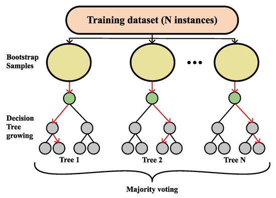
Figure 3.
Visualization of the Random Forest classification process.
The bagging approach is used for producing the tree, i.e., by generating random slices of the training sets using substitution, which means that some slices can be selected more than once and others not at all [56]. Given a particular training set S, generated classifiers toss a vote, thus making a bagged predictor and, at the same time, for every pair from the training set and for every that did not contain , votes from are set aside as out-of-the-bag classifiers [51]. Commonly, a partition of samples is on the training set by taking two-thirds for tree training and leaving one-third for inner cross-validation, thus removing the need for cross-validation or a separate test set [56]. The user is the one defining the number of trees and other hyper-parameters that the algorithm uses for independent tree creation performed without any pruning, where the key is to have a low bias and high variance, and the splitting of each node is based on a user-defined number of features that are randomly chosen [52]. In the end, the final classification is obtained by majority vote, i.e., the instance is classified into the class having the most votes over all trees in the forest [54].
Aiming to produce the best classification accuracy, in this research, hyper-parameter tuning has been performed by utilizing the GridSearchCV class from the scikit-learn library with five-fold cross-validation.
This is performed following the above reasoning for making a structure for each particular tree. By controlling the hyper-parameters, one can supervise the architecture and size of the forest (e.g., the number of trees (n_estimators)) along with the degree of randomness (e.g., max_features) [52]. Therefore, for every frame size, the hyper-parameters presented in Table 3 were tested, resulting in a separate RF model for each of the frame sizes, as presented in Table 4.
Table 3.
Tested Hyper-parameters for Random Forest.
Table 4.
Grid search results of RF Hyper-parameters for a particular frame size.
4. Results and Comparison
For ILCM, Neural Network and Random Forest, the same data were used to make a comprehensive performance comparison. To provide a comprehensive classifier performance comparison, several measures were taken into account. First, to compare the performance of each classifier as a Machine Learning model, the accuracy measure was taken (since it is a standard metric for evaluation of a classifier), this being the categorical accuracy. Categorical accuracy is a Keras built-in metric that calculates the result by finding the largest percentage from the prediction and then compares it to the actual result. If the largest percentage matches the index of 1, then the measured accuracy increases. If it does not match, the accuracy goes down. Our experimental results point out that RF has out-preformed the NN model in the classification task, as shown in Table 5, but this measure alone is not enough to determine which of the two ML models would be preferred for utilization in the scenario of tag estimation. Therefore, due to the nature of the problem of tag estimation, we have considered Mean Absolute Errors (MAE) and Absolute Errors (AE) as measures of classifier performance (see Equations (7) and (8), respectively). An accumulated estimation error will degrade the whole performance [57], meaning that the overall smaller MAE and AE for a classifier would determine the overall estimator efficiency, i.e., better system throughput. For the approximated number of tags and the exact number of tags n, MAE is defined as:
Table 5.
Classification accuracy of NN, RF and the ILCM model for a particular frame size.
For every frame size, AE was calculated as:
As can be noticed from Table 5, as frame size rises, the accuracy decreases for all of the three compared models. Furthermore, Random Forest seems to outperform other classifiers for the most challenging task for . Furthermore, ILCM performed similarly to NN and RF for smaller frame sizes.
On the other hand, the results presented in Table 6 indicate that the Neural Network model produces error rates comparable to RF, although RF has better accuracy. What is more, for the largest frame size, NN will have an overall smaller MAE, as can be seen from Table 6 for frame sizes and . Overall, both Machine Learning classifiers perform substantially better than the ILCM model.
Table 6.
MAE of NN, RF and the ILCM model for a particular frame size.
This observation is further emphasized in the calculations of Absolute Errors of classification for RF, NN and the ILCM model. AE was derived for every frame size, and the histograms presented in Figure 4 provide a pictorial comparison of the errors. As can be seen from Figure 4a, for smaller frame sizes, the NN model performs quite complementary to the RF model, but for the largest frame size, the NN (see Figure 4c) will have an overall smaller AE. These histograms are consistent with the MAE results from Table 6, confirming that the NN classifies values nearer to the true values of the number of tags n. This observation is important for estimating the length of the next frame because the closer the estimated number of interrogating tags is to the actual number of tags, the better the frame size setting. Incorrect estimates of the total number of tags result in lower throughput. Results from this analysis show that, in comparison to the RF model, the NN model is generally “closer” to the real tag number.
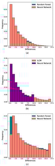
Figure 4.
Comparison of absolute errors for Neural Network, Random Forest and ILCM model for frame sizes (a) , (b) and (c) .
The overall goal is to reach maximum throughput, and this cannot be achieved if the frame size adaptation is inadequate. The development of an effective and simple tag estimator is burdened by the variables that must be taken into account, i.e., the frame size, the number of successful slots, and the number of collisions or empty slots. As was stated in Section 2, the major drawbacks of current estimators lie in their estimation capabilities, computational complexity and memory demands. Therefore, to achieve a better setting of the next frame size, the focus of the estimation should be on the variable that contributes the most to the overall proficiency of the system [23]. Based on the obtained results, one final measure was performed, i.e., a comparison of throughput for the NN model, ILCM and Optimal model. The Optimal being used as the benchmark is the one where the frame adaptation was set by the known number of tags. Results of the comparison are presented for the scenario of frame size realizations and are exhibited in Figure 5. As can be observed from Figure 5, the Neural Network model is close to the optimal one and outperforms the state-of-the-art ILCM model. This is particularly shown as the tag number increases, as can be seen in Figure 5b.
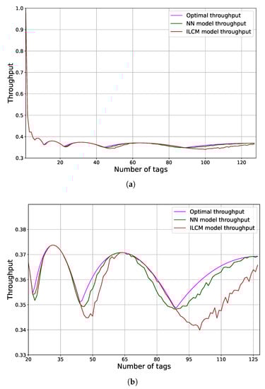
Figure 5.
Comparison of throughput for the NN model, ILCM and Optimal model for the scenario of frame size realizations. (a) Throughput for the NN model, ILCM and Optimal model; (b) Throughput for the NN model, ILCM and Optimal model for a larger number of tags.
Based on the result of this examination of the performance of classifiers and comparison to the ILCM model, architectures of the Neural Network models were selected for further utilization.
5. Mobile RFID Reader—Implementation Feasibility
5.1. Current State-of-the-Art
In recent years, there has been an evident effort to enable the execution of Neural Networks on low-power and limited-performance embedded devices, such as microcontrollers (MCU) and computer boards [58]. The most common benefit that this approach can bring is not needing to transmit data (e.g., radio) to a remote location for computation. With the local implementation of ML capabilities on the MCU-like devices, everything can be executed on a device itself, thus saving the power and time that would be used for data transmission. The sensitivity of the data collected and sent to the remote device also raises concerns about expected security. With this approach, IoT devices that locally run trained ML models significantly reduce the amount of data exchanged with the server through secured or unsecured communication channels. While keeping most of the collected data on the local embedded system, some of the aforementioned privacy concerns are reduced [59]. Researchers are increasingly working on adapting existing embedded Machine Learning algorithms or applications on MCU-like devices, which were previously only possible on high-performance computers [60,61,62].
Led by the idea of implementing ML on embedded systems, several IT industry giants have released support for such devices. As a notable example, Google has released the TensorFlow Lite platform, which enables the user to convert TensorFlow Neural Network (NN) models, which were commonly trained for high-performance computers (e.g., Personal Computers), into a reduced model that can be stored and executed on compatible resource-constrained machines [63]. With a similar idea, Microsoft has published EdgeML, which is also designed to work on common Edge Devices [64], and even reported to work on 8-bit AVR-based Arduino (which holds only 2 KB of RAM and 32 KB of FLASH memory) on common single-board computers, such as the Raspberry Pi family. Such an example is that the same ML model (e.g., produced by TensorFlow Lite library), of course, if device resources allow it, can be executed on a microcontroller (running on Arm Cortex-M7 MCU at 600 MHz and only 51KB RAM) and computer board (e.g., Raspberry Pi4B running on quad-core Cortex-A72 1.5 GHz and 4 GB RAM). Power consumption and possible autonomy on batteries, which is a common requirement for some IoT devices, prefer microcontroller implementation (typical 3 A/5 V for RaspberryPi4 vs. 0.1 A/3.3 V typical for Arm Cortex-M7-based MCU), and for this reason, the following text is focused on ML implementation on microcontrollers with comments on implementation on computer boards. Some semiconductor manufacturers have notably supported the effort to implement ML capabilities in MCU devices. STM has released X-Cube-AI with deep learning capabilities on STM 32-bit microcontrollers [65]. An open-source library Microcontroller Software Interface Standard Neural Network (CMSIS-NN), published by ARM enables today’s most popular series of Cortex-M processors’ execution of ML models [66]. Another interesting example can be seen by third-party microcontroller board manufacturer OpenMV [67]. They produce an OpenMV microcontroller board (based on Arm Cortex-M7 MCU), which is a smart vision camera that is capable of executing complex machine vision algorithms for a low-cost device (typically below 80 USD). The common bottleneck of current microcontroller boards that run deep CNN is a relatively low amount of RAM, which stores NN weights and data. OpenMV H7plus board overcomes this limitation by adding another 32 MB SDRAM in addition to 1 MB RAM, which already came embedded with the microcontroller itself. Additional RAM, in turn, enables the microcontroller to store and run several complex NN models, a task that is commonly impossible on standard MCU-s and can be executed on more complex computer boards, such as the Raspberry Pi family of computer boards. Today’s increasing demand for ML-enabled embedded end-devices, constant improvement in computing power and affordability would introduce new industry standards for smart cities and smart homes.
5.2. Experimental Setup
Common microcontroller boards, as compared to dedicated Personal Computers, are exceptionally bad with floating number calculations (in terms of execution times) as they are designed to work flawlessly with peripheral components rather than execute complex calculations. TensorFlow library can be configured to use 32-bit floating-point data types in a model for both data and weights, which generates a large model. MCU-compatible models implement an approach where integer numbers (8-bit or 16-bit) are used instead of floating-point numbers in calculations, which would considerably decrease the model size but dramatically increase execution speed. The original model (with 32-bit or 64-bit weights) can be executed on a microcontroller, of course, if the model size is small enough for the microcontroller’s available RAM, but the full power of TFLiteConverter will not be used. TensorFlow Lite library for microcontrollers allows us to optimize a pre-trained Neural Network model to a selected microcontroller and implement it on the device. This ability is possible only with smart quantization, which, in turn, approximates 32-bit floating-point values into either 16-bit float-point values or 8-bit integer values. In some scenarios (such as in most complex models presented in this work), there is an evident loss in inaccuracy, which is, on the other hand, greatly compensated by a reduction in memory requirements and improvement in execution times. Finally, for some models, quantization makes all the difference if the model can or cannot be run on a memory-restricted microcontroller. TFLiteConverter, which is part of the TFLite library, can offer several optimization options; float16 quantization of weights and inputs that cut the original model size in just half, with a barely visible reduction in accuracy, dynamic range quantization where weights are 8-bit while activations are floating-point and computation is still performed in floating-point operations (optimal trade-off for some low-performance but still capable computer boards). The third optimization option showed to be ideal for low-power microcontroller devices, with forces of full integer quantization, where weight and activations are both 8-bit and all operations are integers. The aforementioned quantization is slightly more complicated than the other approaches, as the converter is required to be fed with a representative dataset before the quantization of the whole model. The data shown in Table 7 provide a simple insight into the accuracy decrease due to the performed quantization for models used in our paper.
Table 7.
Model accuracy before and after quantization.
It can be observed that a decrease in accuracy is observable for the two most complex NN architectures (L = 128 and L = 256), while for the least complex NN architectures (L = 4 and L = 8) the loss due to quantization is merely measurable. The loss inaccuracy for the two most complex architectures is possibly the result of output quantization where more than 256 classes are possible (notably 512 for L = 128 and 1024 for L = 256).
After the quantized model is created, a file containing the model that the microcontroller will understand is created. The Linux command tool xxd takes a data file and outputs a text-based hex dump, which we copy-paste as a c array, and add to a microcontroller project source code (as an additional header file).
5.3. MCU Hardware
The Teensy 4.0 microcontroller board features an ARM Cortex-M7 processor with an NXP iMXRT1062 chip clocked up to 600 MHz without additional cooling (faster stable speeds are possible with an additional heatsink). To our knowledge, this computer board is the fastest microcontroller board available on today’s market that can be used out-of-the-box [68] for complex calculations. When running at 600 MHz, Teensy 4.0 consumes approximately 100 mA current (at 3.3 V supplied voltage), considerably more than some common microcontrollers, such as the Arduino AVR family, but significantly less than any desktop computers or computer boards. The Teensy 4.0 microcontroller features 1024K RAM (of which 512K is tightly coupled) available for storing local data. The ML model is stored in FLASH memory during programming, after which it is read in whole or segment-per-segment into the RAM (this option is library dependant and tweakable). Another microcontroller board in the ML domain that was considered was AMR M3-based Arduino Due, which sports an Atmel SAM3X8E microcontroller clocked at 84 Mhz and offers a significantly smaller amount of RAM (96 KB) [69]. Considerably lower amounts of available RAM for this microcontroller can make it unusable in executing more complex ML models, where constant reading data from slower FLASH memory can lead to significantly longer execution times. The third microcontroller board that was initially considered was the popular STM32F103C8T6 (known as “blue pill”), which is also based on the Arm Cortex-M3 microcontroller. This board clocks 72 MHz but holds only 20 KB of RAM and 64 KB of FLASH memory, which makes holding and execution of most of our opposed NN models impossible citexcube. All three devices that have been tested are presented in Figure 6.
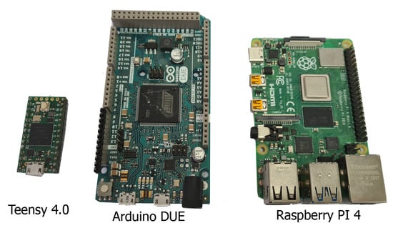
Figure 6.
Devices used in the test: Teensy 4.0 (left), Arduino DUE (center) and Raspberry Pi4 (right). Source: Own photo.
To provide better insight into the microcontroller’s performance in executing proposed NN models, the same quantized TensorFlow models were tested on a common computer board. A Raspberry Pi 4B computer board was used, which holds a quad-core Cortex-A72 1.5 GHz SOC with 4 GB of RAM, and runs Raspian desktop OS with kernel version 5.10. With simplicity in mind, all coding for the microcontroller side was performed in Arduino IDE [70], which offers a simple and intuitive interface and the availability of numerous additional libraries for a project extension. The ML model was implemented to the project by adding a hexdump file as an additional header file, which is then converted into a binary format and transferred to the microcontroller’s FLASH memory during programming. The Raspberry Pi computer uses a simple Python script with an additional TFLite interpreter library.
Several proposed model architectures on the Teensy 4.0 microcontroller board were trained that have been considered as the optimal solution for executing the proposed NN models. The presented analysis aims to indicate the real limits of the NN architecture that can be fluently run on selected hardware. ANN layers’ configuration was kept intact, while the complexity of the model was achieved by increasing the number of neurons in the third and fifth layers. By utilizing a microcontroller-integrated timer, the average ANN execution time has been measured on the microcontroller. Another interesting piece of information obtained was the quantized model size and amount of RAM commonly assigned for storing global variables after initial programming. Please note that microcontrollers usually do not possess the possibility of measuring free RAM space during execution, as compared to computers. The used library offers some tweaking of tensor size, which may reduce or increase available RAM size and consequently affect execution time, but we kept this option on default for all tested models and all devices. It is recommended to keep at least 10 % of available RAM for local variables for stable performance. The results for all six models’ execution times and model size on Teensy 4.0 ARM Cortex M7 microcontroller, Arduino DUE ARM Cortex M3 microcontroller and the Raspberry Pi4 computer board are listed in Table 8.
Table 8.
Model performance on Teensy 4.0 MCU, Arduino DUE and Raspberry Pi4.
5.4. Discussion
As can be observed from Table 8, increasing the number of neurons in hidden layers (notably hidden layers 3 and 5) and in output layers increases the model size and prolongs execution. As an example, comparing models for L = 4 and with the model for L = 16, which have exactly twice as many neurons as in layers 3 and 5, the total model size increases by a factor of 1.5, while the execution time on the Teensy 4.0 microcontroller observes an increase of 2.2. The last presented model (L = 256) features an increase in model size by a factor of 65 and in execution time by a factor of 75, as compared to the simplest model (L = 4). It is worth mentioning that the last model represents an example of the most complex ANN model that our microcontroller can hold, where after importing it to the microcontroller, only 13% of the RAM was free for local variables. We also observed that increasing the depth and/or increasing the number of neurons per layer of an NN poses a significant memory demand, which can be afforded only by high-end edge devices (e.g., Raspberry Pi). The average execution time for the most complex exemplary model was 1.7 ms, which is surprisingly fast for this type of device and can offer real-time performance. The ARM Cortex M3-based Arduino DUE behaved similarly to the Teensy 4.0 microcontroller with significantly longer execution times (41 times slower on the simplest model and 67 times slower on the most complex model). The execution of the most complex model took 111 ms, which makes it impractical for some real-time scenarios. Execution times on the Raspberry Pi4 computer varied greatly (due to non-real-time OS architecture) and surprisingly showed to be much slower for less complex models (up to L = 32). For more complex models, Raspberry Pi was able to benefit from its enormous computing power, and the most complex model executed in 0.6 ms, which, when compared to Teensy 4.0, is not significantly better to persuade us to use computer boards instead of the microcontroller. This once more proves that if the loss in accuracy due to quantization is acceptable, the only real limitation is available RAM and FLASH memory on the used microcontroller.
In some scenarios, RF can offer better or comparable results to deep NN with only a fraction of the execution time required on MCU [71]. As the aim of our study was to increase throughput, which is achieved by better estimating the number of interrogating tags, which is best performed by the NN model, only the NN model was considered for implementation on the microcontrollers. Additionally, NN models can offer numerous optimization and quantization possibilities, which is worth further investigation.
Based on the overall result, one final observation is made. As can be noticed in Figure 5, the for ILCM and NN is quite different. Such diversity is a result of the ILCM’s interpolation, even though it contributes to lower computation complexity. When examining the worst case for both models, i.e., frame size , the Neural Network model reaches in contrast to . This results in a difference of , which is approximately 6 successful slots per given frame. The reader setting determines the execution time per frame and such a time cost needs to be compared with the time for a successful tag read, i.e., successful slot time. Based on empirical evidence from research studies, such as the ones in [72], the time for standard reader setting in a general scenario is 3 ms. Therefore, the read tags that are marked as Neural Network computational burden are equal to 1.7 ms/3 ms = 0.57.
5.5. Limitations to the Study
There are a few noteworthy limitations to this study. First, this study is based on data obtained from Monte Carlo simulations. Although simulated data are not the same as experimentally measured data, the Monte Carlo method creates sampling distributions of relevant statistics and can be efficiently implemented on a computer. What is more, the method allows the creation of the desired amount of sample data. The number of sample data used for training and testing ML algorithms is a crucial parameter when testing algorithms’ performance. Furthermore, by using data obtained by Monte Carlo simulations, this research has remained consistent with the methodology presented in research [8] regarding the ILCM model.
Secondly, more frame sizes could have been considered to obtain better insight into models’ performance and as such, they can be considered in future work. Thirdly, other Machine Learning classifiers cloud be employed, tested and compared to the utilized Random Forest and Neural Network.
Finally, as one of the aims of this study was to find a model that can be executed in resource-constrained microcontrollers, we were bounded by the relative “simplicity” of the proposed models (e.g., the model presented in this research is based on multilayer perceptron), while more complex NN models were not considered at this moment (e.g., recurrent networks, convolutional network), which is also planned for future work.
6. Conclusions
The research presented in this study aimed to explore how broadly utilized Machine Learning classifiers can be applied for tag number estimation within ALOHA-based RFID systems to increase the systems’ throughput. The strengths and weaknesses of each of the models are explored on a particularly designed dataset obtained from Monte Carlo simulations. The state-of-the-art algorithm, namely the Improved Linearized Combinatorial Model (ILCM) for tag estimation, is used to compare the performance of the ML algorithms, namely Neural Network and Random Forest.
The obtained results demonstrate that the Neural Network classifier outperforms the ILCM model and achieves higher throughput.
Furthermore, this study tested to see if ML classifiers can be deployed on mobile RFID readers, aiming to maximize tag identification performance with suitable energy and processing demands. Experimental results show that the NN model architecture can be executed on resource-limited MCUs. These results imply that the conventional RFID readers may be equipped with Machine Learning classifiers that use the maximum of the available information acquired from Monte Carlo simulations. The overall results prove that the execution time on MCU is enough to meet protocol needs, keep up with the latency and improve system throughput.
Author Contributions
Conceptualization, L.D.R., I.S. and P.Š.; methodology, L.D.R., I.S. and P.Š.; software, L.D.R. and I.S.; validation, L.D.R., I.S., P.Š. and K.Z.; formal analysis, L.D.R. and P.Š.; investigation, L.D.R. and I.S.; resources, L.D.R., I.S. and K.Z.; data curation, L.D.R.; writing—original draft preparation, L.D.R., I.S., P. Š., K.Z. and T.P.; writing—review and editing, L.D.R., I.S., P.Š., K.Z. and T.P.; visualization, L.D.R., T.P. and I.S.; supervision, P.Š. and T.P. All authors have read and agreed to the published version of the manuscript.
Funding
This research was funded by the Croatian Science Foundation under the project “Internet of Things: Research and Applications”, UIP-2017-05-4206.
Conflicts of Interest
The authors declare no conflict of interest.
Abbreviations
The following abbreviations are used in this manuscript:
| IoT | Internet of Things |
| RFID | Radio Frequency Identification |
| WIPT | Wireless Information and Power Transfer |
| DFSA | Dynamic Framed Slotted ALOHA |
| TDMA | Time-Division multiple-access |
| ILCM | Improved Linearized Combinatorial model |
| ML | Machine Learning |
| DT | Decision Tree |
| k-NN | k-Nearest Neighbour |
| SVM | Support Vector Machine |
| RF | Random Forest |
| DL | Deep Learning |
| ANN | Artificial Neural Networks |
| NN | Neural Network |
| ReLU | Rectified Linear Unit |
| SGD | Stochastic Gradient Descent |
| Adam | Adaptive Moment Optimization |
| RMSProp | Root Mean Square Propagation |
| MAE | Mean Absolute Errors |
| CMSIS-NN | Microcontroller Software Interface Standard Neural Network |
| MCU | microcontrollers |
References
- Cui, L.; Zhang, Z.; Gao, N.; Meng, Z.; Li, Z. Radio Frequency Identification and Sensing Techniques and Their Applications—A Review of the State-of-the-Art. Sensors 2019, 19, 4012. [Google Scholar] [CrossRef] [PubMed]
- Santos, Y.; Canedo, E. On the Design and Implementation of an IoT based Architecture for Reading Ultra High Frequency Tags. Information 2019, 10, 41. [Google Scholar] [CrossRef]
- Landaluce, H.; Arjona, L.; Perallos, A.; Falcone, F.; Angulo, I.; Muralter, F. A Review of IoT Sensing Applications and Challenges Using RFID and Wireless Sensor Networks. Sensors 2020, 20, 2495. [Google Scholar] [CrossRef]
- Dobkin, D.D. The RF in RFID; Elsevier: Burlington, MA, USA, 2008. [Google Scholar]
- Škiljo, M.; Šolić, P.; Blažević, Z.; Patrono, L.; Rodrigues, J.J.P.C. Electromagnetic characterization of SNR variation in passive Gen2 RFID system. In Proceedings of the 2017 Ninth International Conference on Ubiquitous and Future Networks (ICUFN), Milan, Italy, 4–7 July 2017; pp. 172–175. [Google Scholar] [CrossRef]
- Šolić, P.; Maras, J.; Radić, J.; Blažević, Z. Comparing Theoretical and Experimental Results in Gen2 RFID Throughput. IEEE Trans. Autom. Sci. Eng. 2017, 14, 349–357. [Google Scholar] [CrossRef]
- EPCglobal Inc. Class1 Generation 2 UHF Air Interface Protocol Standard; Technical Report; EPCglobal Inc.: Wellington, New Zealand, 2015. [Google Scholar]
- Šolić, P.; Radić, J.; Rožić, N. Energy Efficient Tag Estimation Method for ALOHA-Based RFID Systems. IEEE Sens. J. 2014, 14, 3637–3647. [Google Scholar] [CrossRef]
- Law, C.; Lee, K.; Siu, K.Y. Efficient Memoryless Protocol for Tag Identification (Extended Abstract); Association for Computing Machinery: New York, NY, USA, 2000. [Google Scholar] [CrossRef]
- Capetanakis, J. Tree algorithms for packet broadcast channels. IEEE Trans. Inf. Theory 1979, 25, 505–515. [Google Scholar] [CrossRef]
- Rodić, L.D.; Stančić, I.; Zovko, K.; Šolić, P. Machine Learning as Tag Estimation Method for ALOHA-based RFID system. In Proceedings of the 2021 6th International Conference on Smart and Sustainable Technologies (SpliTech), Bol and Split, Croatia, 8–11 September 2021; pp. 1–6. [Google Scholar] [CrossRef]
- Schoute, F. Dynamic Frame Length ALOHA. IEEE Trans. Commun. 1983, 31, 565–568. [Google Scholar] [CrossRef]
- Škiljo, M.; Šolić, P.; Blažević, Z.; Rodić, L.D.; Perković, T. UHF RFID: Retail Store Performance. IEEE J. Radio Freq. Identif. 2021, 6, 481–489. [Google Scholar] [CrossRef]
- Chen, W. An Accurate Tag Estimate Method for Improving the Performance of an RFID Anticollision Algorithm Based on Dynamic Frame Length ALOHA. IEEE Trans. Autom. Sci. Eng. 2009, 6, 9–15. [Google Scholar] [CrossRef]
- Vogt, H. Efficient object identification with passive RFID tags. In Proceedings of the International Conference on Pervasive Computing, Zürich, Switzerland, 26–28 August 2002; pp. 98–113. [Google Scholar]
- Šolić, P.; Radić, J.; Rozić, N. Linearized Combinatorial Model for optimal frame selection in Gen2 RFID system. In Proceedings of the 2012 IEEE International Conference on RFID (RFID), Orlando, FL, USA, 3–5 April 2012; pp. 89–94. [Google Scholar] [CrossRef]
- Vahedi, E.; Wong, V.W.S.; Blake, I.F.; Ward, R.K. Probabilistic Analysis and Correction of Chen’s Tag Estimate Method. IEEE Trans. Autom. Sci. Eng. 2011, 8, 659–663. [Google Scholar] [CrossRef]
- Arjona, L.; Landaluce, H.; Perallos, A.; Onieva, E. Scalable RFID Tag Estimator with Enhanced Accuracy and Low Estimation Time. IEEE Signal Process. Lett. 2017, 24, 982–986. [Google Scholar] [CrossRef]
- Delgado, M.; Vales-Alonso, J.; Gonzalez-Castao, F. Analysis of DFSA anti-collision protocols in passive RFID environments. In Proceedings of the 2009 35th Annual Conference of IEEE Industrial Electronics, Porto, Portugal, 3–5 November 2009; pp. 2610–2617. [Google Scholar] [CrossRef]
- Vales-Alonso, J.; Bueno-Delgado, V.; Egea-Lopez, E.; Gonzalez-Castano, F.J.; Alcaraz, J. Multiframe Maximum-Likelihood Tag Estimation for RFID Anticollision Protocols. IEEE Trans. Ind. Inform. 2011, 7, 487–496. [Google Scholar] [CrossRef]
- Wang, S.; Aggarwal, C.; Liu, H. Using a Random Forest to Inspire a Neural Network and Improving on It. In Proceedings of the 2017 SIAM International Conference on Data Mining (SDM), Houston, TX, USA, 27–29 April 2017; pp. 1–9. [Google Scholar] [CrossRef]
- Filho, I.E.D.B.; Silva, I.; Viegas, C.M.D. An Effective Extension of Anti-Collision Protocol for RFID in the Industrial Internet of Things (IIoT). Sensors 2018, 18, 4426. [Google Scholar] [CrossRef] [PubMed]
- Radić, J.; Šolić, P.; Škiljo, M. Anticollision algorithm for radio frequency identification system with low memory requirements: NA. Trans. Emerg. Telecommun. Technol. 2020, 31, e3969. [Google Scholar] [CrossRef]
- Boovaraghavan, S.; Maravi, A.; Mallela, P.; Agarwal, Y. MLIoT: An End-to-End Machine Learning System for the Internet-of-Things. In Proceedings of the International Conference on Internet-of-Things Design and Implementation, Charlottesville, VA, USA, 18–21 May 2021; IoTDI ’21. pp. 169–181. [Google Scholar] [CrossRef]
- Mitchell, T.M. Machine Learning; McGraw-Hill: New York, NY, USA, 1997. [Google Scholar]
- Sarkar, D.; Bali, R.; Sharma, T. Practical Machine Learning with Python: A Problem-Solver’s Guide to Building Real-World Intelligent Systems, 1st ed.; Apress: New York, NY, USA, 2017. [Google Scholar]
- Zantalis, F.; Koulouras, G.; Karabetsos, S.; Kandris, D. A Review of Machine Learning and IoT in Smart Transportation. Future Internet 2019, 11, 94. [Google Scholar] [CrossRef]
- Hussain, F.; Hussain, R.; Hassan, S.A.; Hossain, E. Machine Learning in IoT Security: Current Solutions and Future Challenges. IEEE Commun. Surv. Tutor. 2020, 22, 1686–1721. [Google Scholar] [CrossRef]
- Dujić Rodić, L.; Perković, T.; Županović, T.; Šolić, P. Sensing Occupancy through Software: Smart Parking Proof of Concept. Electronics 2020, 9, 2207. [Google Scholar] [CrossRef]
- Sen, P.C.; Hajra, M.; Ghosh, M. Supervised Classification Algorithms in Machine Learning: A Survey and Review. In Emerging Technology in Modelling and Graphics; Mandal, J.K., Bhattacharya, D., Eds.; Springer: Singapore, 2020; pp. 99–111. [Google Scholar]
- Soofi, A.A.; Awan, A. Classification Techniques in Machine Learning: Applications and Issues. J. Basic Appl. Sci. 2017, 13, 459–465. [Google Scholar] [CrossRef]
- Zhu, X.X.; Tuia, D.; Mou, L.; Xia, G.; Zhang, L.; Xu, F.; Fraundorfer, F. Deep Learning in Remote Sensing: A Comprehensive Review and List of Resources. IEEE Geosci. Remote. Sens. Mag. 2017, 5, 8–36. [Google Scholar] [CrossRef]
- LeCun, Y.; Bengio, Y.; Hinton, G. Deep Learning. Nature 2015, 521, 436–444. [Google Scholar] [CrossRef]
- Kotsiantis, S.B.; Zaharakis, I.; Pintelas, P. Supervised machine learning: A review of classification techniques. Emerg. Artif. Intell. Appl. Comput. Eng. 2007, 160, 3–24. [Google Scholar]
- Nikam, S.S. A comparative study of classification techniques in data mining algorithms. Orient. J. Comput. Sci. Technol. 2015, 8, 13–19. [Google Scholar]
- Charoenpong, J.; Pimpunchat, B.; Amornsamankul, S.; Triampo, W.; Nuttavut, N. A Comparison of Machine Learning Algorithms and their Applications. Int. J. Simul. Syst. Sci. Technol. 2019, 20, 8. [Google Scholar]
- Mothkur, R.; Poornima, K. Machine learning will transfigure medical sector: A survey. In Proceedings of the 2018 International Conference on Current Trends towards Converging Technologies (ICCTCT), Coimbatore, India, 1–3 March 2018; pp. 1–8. [Google Scholar]
- Cutler, A.; Cutler, D.; Stevens, J. Random Forests. In Ensemble Machine Learning; Springer: Boston, MA, USA, 2012; Volume 45, pp. 157–176. [Google Scholar] [CrossRef]
- Paul, A.; Mukherjee, D.P.; Das, P.; Gangopadhyay, A.; Chintha, A.R.; Kundu, S. Improved Random Forest for Classification. IEEE Trans. Image Process. 2018, 27, 4012–4024. [Google Scholar] [CrossRef]
- Kulkarni, V.Y.; Sinha, P.K. Pruning of Random Forest classifiers: A survey and future directions. In Proceedings of the 2012 International Conference on Data Science Engineering (ICDSE), Kerala, India, 18–20 July 2012; pp. 64–68. [Google Scholar] [CrossRef]
- Lipton, Z.C. A Critical Review of Recurrent Neural Networks for Sequence Learning. arXiv 2015, arXiv:1506.00019. [Google Scholar]
- Ng, A.Y.; Jordan, M.I. On Discriminative vs. Generative Classifiers: A comparison of logistic regression and naive Bayes. In Proceedings of the Advances in Neural Information Processing Systems 14 (NIPS 2001), Vancouver, BC, Canada, 3–8 December 2001; Dietterich, T.G., Becker, S., Ghahramani, Z., Eds.; MIT Press: Cambridge, MA, USA, 2001; pp. 841–848. [Google Scholar]
- Joo, R.; Bertrand, S.; Tam, J.; Fablet, R. Hidden Markov Models: The Best Models for Forager Movements? PLoS ONE 2013, 8, e71246. [Google Scholar] [CrossRef]
- Zhang, G.P. Neural networks for classification: A survey. IEEE Trans. Syst. Man, Cybern. Part C Appl. Rev. 2000, 30, 451–462. [Google Scholar] [CrossRef]
- Roßbach, P. Neural Networks vs. Random Forests—Does It Always Have to Be Deep Learning; Frankfurt School of Finance and Management: Frankfurt am Main, Germany, 2018. [Google Scholar]
- Biau, G.; Scornet, E.; Welbl, J. Neural random forests. Sankhya A 2019, 81, 347–386. [Google Scholar] [CrossRef]
- NVIDIA; Vingelmann, P.; Fitzek, F.H. CUDA, Release: 11.2. 2021. Available online: https://developer.nvidia.com/cuda-toolkit (accessed on 21 July 2021).
- Provoost, J.; Wismans, L.; der Drift, S.V.; Kamilaris, A.; Keulen, M.V. Short Term Prediction of Parking Area states Using Real Time Data and Machine Learning Techniques. arXiv 2019, arXiv:1911.13178. [Google Scholar]
- Dongare, A.D.; Kharde, R.R.; Kachare, A.D. Introduction to Artificial Neural Network. Int. J. Eng. Innov. Technol. 2012, 2, 189–194. [Google Scholar]
- Hayou, S.; Doucet, A.; Rousseau, J. On the Impact of the Activation function on Deep Neural Networks Training. In Proceedings of the 36th International Conference on Machine Learning, Long Beach, CA, USA, 9–15 June 2019; Chaudhuri, K., Salakhutdinov, R., Eds.; 2019; Volume 97, pp. 2672–2680. [Google Scholar]
- Breiman, L. Random Forests. Mach. Learn. 2001, 45, 5–32. [Google Scholar] [CrossRef]
- Probst, P.; Wright, M.N.; Boulesteix, A.L. Hyperparameters and tuning strategies for random forest. Wires Data Min. Knowl. Discov. 2019, 9, e1301. [Google Scholar] [CrossRef]
- Biau, G.; Scornet, E. A random forest guided tour. Test 2016, 25, 197–227. [Google Scholar] [CrossRef]
- Prinzie, A.; Van den Poel, D. Random Forests for multiclass classification: Random MultiNomial Logit. Expert Syst. Appl. 2008, 34, 1721–1732. [Google Scholar] [CrossRef]
- Oshiro, T.M.; Perez, P.S.; Baranauskas, J.A. How Many Trees in a Random Forest? In Proceedings of the Machine Learning and Data Mining in Pattern Recognition, Berlin, Germany, 20–21 July 2012; Perner, P., Ed.; Springer: Berlin/Heidelberg, Germany, 2012; pp. 154–168. [Google Scholar]
- Belgiu, M.; Drăguţ, L. Random forest in remote sensing: A review of applications and future directions. ISPRS J. Photogramm. Remote. Sens. 2016, 114, 24–31. [Google Scholar] [CrossRef]
- Su, J.; Sheng, Z.; Leung, V.C.M.; Chen, Y. Energy Efficient Tag Identification Algorithms For RFID: Survey, Motivation And New Design. IEEE Wirel. Commun. 2019, 26, 118–124. [Google Scholar] [CrossRef]
- Sakr, F.; Bellotti, F.; Berta, R.; De Gloria, A. Machine Learning on Mainstream Microcontrollers. Sensors 2020, 20, 2638. [Google Scholar] [CrossRef]
- Shi, W.; Cao, J.; Zhang, Q.; Li, Y.; Xu, L. Edge Computing: Vision and Challenges. IEEE Internet Things J. 2016, 3, 637–646. [Google Scholar] [CrossRef]
- Magno, M.; Cavigelli, L.; Mayer, P.; von Hagen, F.; Benini, L. FANNCortexM: An Open Source Toolkit for Deployment of Multi-layer Neural Networks on ARM Cortex-M Family Microcontrollers: Performance Analysis with Stress Detection. In Proceedings of the 2019 IEEE 5th World Forum on Internet of Things (WF-IoT), Limerick, Ireland, 15–18 April 2019; pp. 793–798. [Google Scholar] [CrossRef]
- Alameh, M.; Abbass, Y.; Ibrahim, A.; Valle, M. Smart Tactile Sensing Systems Based on Embedded CNN Implementations. Micromachines 2020, 11, 103. [Google Scholar] [CrossRef]
- Sharma, R.; Biookaghazadeh, S.; Li, B.; Zhao, M. Are Existing Knowledge Transfer Techniques Effective for Deep Learning with Edge Devices? In Proceedings of the 2018 IEEE International Conference on Edge Computing (EDGE), San Francisco, CA, USA, 2–7 July 2018; pp. 42–49. [Google Scholar] [CrossRef]
- TensorFlow Lite. Available online: http://www.tensorflow.org/lite (accessed on 21 July 2021).
- EdgeML Machine LEARNING for Resource-Constrained Edge Devices. Available online: https://github.com/Microsoft/EdgeML (accessed on 21 July 2021).
- STM32CubeMX—STMicroelectronics, X-CUBE-AI—AI. Available online: https://http://www.st.com/en/embedded-software/x-cube-ai.html (accessed on 21 July 2021).
- CMSIS NN Software Library. Available online: https://arm-software.github.io/CMSIS_5/NN/html/index.html (accessed on 21 July 2021).
- COepnMV. Available online: https://openmv.io (accessed on 21 July 2021).
- Teensy 4.0 Development Board. Available online: https://www.pjrc.com/store/teensy40.html (accessed on 21 July 2021).
- Atmel SAM3X8E ARM Cortex-M3 MCU. Available online: http://ww1.microchip.com/downloads/en/DeviceDoc/Atmel-11057-32-bit-Cortex-M3-Microcontroller-SAM3X-SAM3A_Datasheet.pdf (accessed on 21 July 2021).
- Arduino IDE. Available online: https://www.arduino.cc/en/software (accessed on 21 July 2021).
- Elsts, A.; McConville, R. Are Microcontrollers Ready for Deep Learning-Based Human Activity Recognition? Electronics 2021, 10, 2640. [Google Scholar] [CrossRef]
- Šolić, P.; Šarić, M.; Stella, M. RFID reader-tag communication throughput analysis using Gen2 Q-algorithm frame adaptation scheme. Int. J. Circuits Syst. Signal Proc. 2014, 8, 233–239. [Google Scholar]
Publisher’s Note: MDPI stays neutral with regard to jurisdictional claims in published maps and institutional affiliations. |
© 2022 by the authors. Licensee MDPI, Basel, Switzerland. This article is an open access article distributed under the terms and conditions of the Creative Commons Attribution (CC BY) license (https://creativecommons.org/licenses/by/4.0/).