3.1. Machine Learning Classifiers for Tag Estimation
The IoT surroundings rich with sensor devices that are interconnected have also yielded the demand for the more efficient monitoring of sensor activities and events [
24]. To support diverse IoT use-case scenarios, Machine Learning has emerged as an essential area of scientific study and employment to enable computers to automatically progress through experience [
25]. Commonly, ML incorporates data analyses and processing followed by training phases to produce “a model”, which is onward tested. The overall goal is to expedite the system to act based on the results and inputs given within the training phase [
26]. For the system to successfully achieve the learning process, distinctive algorithms and models along with data analyses are employed to extract and gain insight into data correlation [
27]. Thus far, Machine Learning has been fruitfully applied to various problems such as regression, classification and density estimation [
28]. Specific algorithms are universally split into disjoint groups known as Unsupervised, Supervised, Semi-supervised and Reinforcement algorithms. The selection of the most appropriate ML algorithm for a specific purpose is performed based on its speed and computational complexity [
27].
Machine Learning applications range from prediction, image processing, speech recognition, computer vision, semantic analysis, natural language processing, as well as information retrieval [
29]. In a problem like the estimation of the tag number based on the provided input, one must consider the most applicable classifiers that can deal with a particular set of data. Currently, classification algorithms have been applied for financial analyses, bio-informatics, face detection, handwriting recognition, image classification, text classification, spam filtering, etc. [
30]. In a classification problem, a targeted label is generally a bounded number of discrete categories, such as in the case of estimating the number of tags. State-of-the-art algorithms for classification incorporate Decision Tree (DT), k-Nearest Neighbour (
k-NN), Support Vector Machine (SVM), Random Forest (RF) and Bayesian Network [
31]. In the last decade, Deep Learning (DL) has manifested itself as a novel ML technique that has efficiently solved problems that have not been overcome by more traditional ML algorithms [
26]. Considered to be one of the most notable technologies of the decade, DL utilizations have obtained remarkable accuracy in various fields such as image and audio-related domains [
26,
32]. DL has the remarkable ability to discover the complex configuration of large datasets using a backpropagation algorithm indicating in what manner the machine’s internal parameters need to be altered to calculate and determine each layer’s representation based on the representation of previous layers [
33]. The essential principle of DL has been displayed throughout growing research performed in Neural Networks or Artificial Neural Networks (ANN). This approach allows for a layered structure of concepts with multiple levels of abstraction, in which every layer of concepts is made from some simpler layers [
26]. Deep Learning has made improvements in problem-solving with regards to discovering intricate configurations of large-sized data and thus has been applied in various domains ranging from image recognition, speech recognition, natural language understanding, sentiment analysis and many more [
33]. Machine Learning classifier performance has been extensively analyzed in the last decade [
34,
35,
36,
37], providing a systematical insight into the classifiers’ key attributes.
Table 1 provides a comparison of the advantages and limitations of commonly utilized ML classifiers.
Tag number estimation can be regarded as a multi-class classification problem. Amongst many classifiers, Random Forest has been considered a simple yet powerful algorithm for classification, successfully applied in numerous problems such as image annotation, text classification, medical data etc. [
38]. RF has been proven to be very accurate when dealing with large datasets; it is robust to noise and has a parallel architecture that makes it faster than other state-of-the-art classifiers [
39]. Furthermore, it is also very efficient in stabilizing classification errors when dealing with unbalanced datasets [
40]. On the other hand, Neural Networks offer great potential for multi-class classification due to their non-linear architecture and prominent approximation proficiency to comprehend tangled input–output relationships between data [
41].
Discriminative models, such as Neural Networks and Random Forest, can model the decision boundary between the classes [
42], thus providing vigorous solutions for non-linear discrimination in high-dimensional spaces [
43]. Therefore, their utilization for classification proposes has proven to be successful and efficient [
44]. Both algorithms are able to model linear as well as complex non-linear relationships. However, Neural Networks have a greater potential here due to their construction [
45]. On the other hand, RF outperforms NN in arbitrary domains, particularly in cases when the underlying data sizes are small, and no domain-specific insight has been used to arrange the architecture of the underlying NN [
21]. Although NN is an expressively rich tool for complex data modeling, they are prone to overfitting on small datasets [
46] and are very time-consuming and computationally intensive [
45]. Furthermore, their performance is frequently sensitive to the specific architectures used to arrange the computational units [
21] in contrast to the computational cost and time of training a Random Forest, requiring much less input preparation [
45]. Finally, although RF needs less hyper-parameter tuning than NN, the acquisitive feature space separation by orthogonal hyper-planes produces typical stair or box-like decision surfaces, which can be beneficial for some datasets but sub-optimal for others [
46].
Following the stated reasoning, Neural Network and Random Forest have been applied in this research for tag number estimation based on the scenarios that occur during slot interrogation.
3.1.1. Experimental Setup
To obtain valuable data for model comparison, Monte Carlo simulations were performed to produce an adequate number of possible scenarios that may happen during the interrogation procedure in DFSA. Detailed elaboration of the mathematical background of the Monte Carlo method that has been applied for this research has been elaborated in research prior to this one and presented in [
11]. The selected approach for Monte Carlo simulations of the distribution of tags in the slots follows the research performed in studies [
8] and [
23]. Simulations were executed for frame sizes
and 256, i.e., for
and 8, where the number of tags was in the range of
(this range was chosen based upon experimental findings elaborated in [
23]). For each of the frame sizes and the number of tags, random 100,000 distributions of
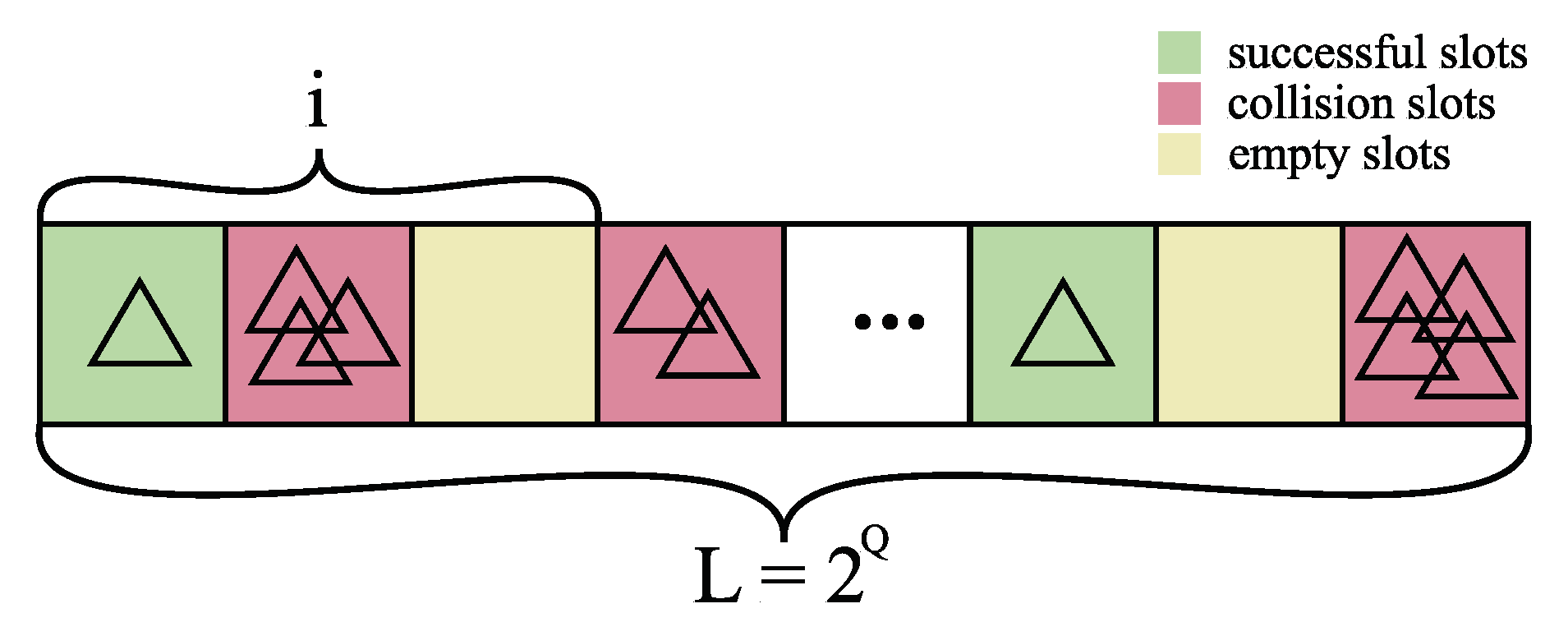
E empty slots, successful slots
S and collision slots
C were realized and are presented in
Table 2.
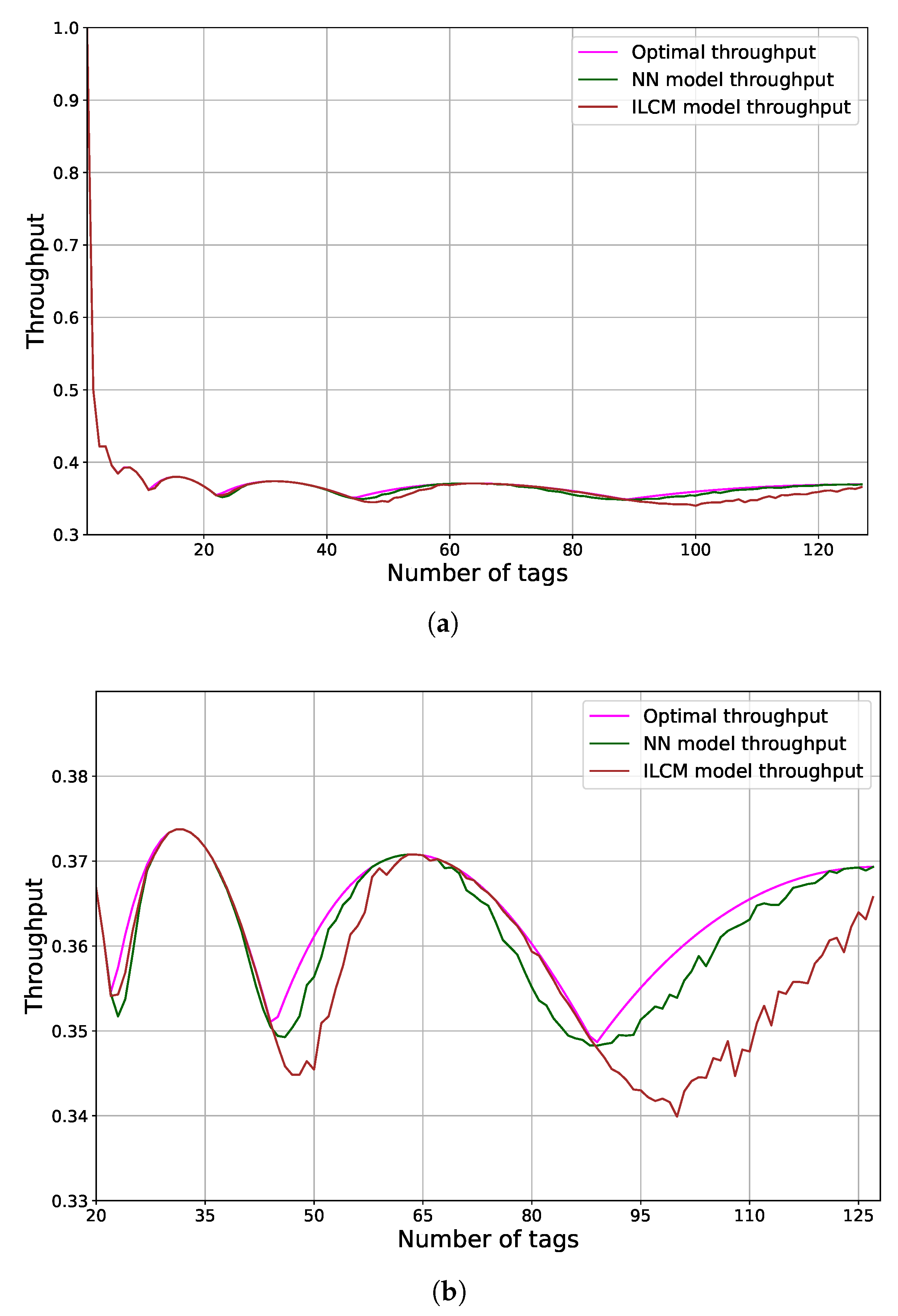
Data obtained from the simulations were given to Neural Network, Random Forest and the ILCM models for adequate performance comparison and analyses of the accuracy of tag estimation.
All of the models and simulations were performed on a dedicated computer for such tasks. To be precise, the machine has an Intel(R) Core(TM) i7-7700HQ@2.80 GHz processor, 16 GB of RAM and NVIDIA GeForce GTX 1050 Ti with 768 existing cores running on a 64-bit Windows 10 operating system. Furthermore, to realize more efficient computing with the GPU, the Deep Neural Network NVIDIA CUDA library (cuDNN) [
47] was applied. The Keras 2.3.1. Python library was employed, which operates on top of a source built upon Tensorflow 2.2.0 with CUDA support for different batch sizes.
3.1.2. Neural Network Model
In general, a Neural Network is made out of an artificial neuron and layer: the input, the hidden layer (or layers) and the output layer are all interconnected [
26], as exhibited in
Figure 2.
Aiming to imitate the behavior of real biological neurons, the course of learning within a NN unfolds through uncovering hidden correlations amongst the sequences of input data throughout layers of neurons. The outputs from neurons in one layer are onward given as inputs to the neurons in the next layer. A formal mathematical definition of an artificial neuron given by Equation (
6) is as follows.
Definition 1. An artificial neuron is the output of the non-linear mapping θ applied to a weighted sum of input values x and a bias β defined as:where represents the matrix of weights and is called an artificial neuron. The weights are appointed considering the inputs’ correlative significance to the other inputs, and the bias ensures a consistent value is added to the mapping to ensure successful learning [
48]. Generally, the mapping
is known as the activation (or transfer) function. Its purpose is to keep the amplitude of the output of the neuron in an adequate range of
or
[
49]. Although activation functions may be linear and non-linear, usually the non-linear ones are more frequently utilized. The most recognizable ones are ordinary Sigmoids or the Softmax function, such as the hyperbolic tangent
, in contrast to Rectified Linear Unit (ReLU) function:
[
33]. The selection of a particular activation function is based on the core problem to be solved by applying the Neural Network [
50].
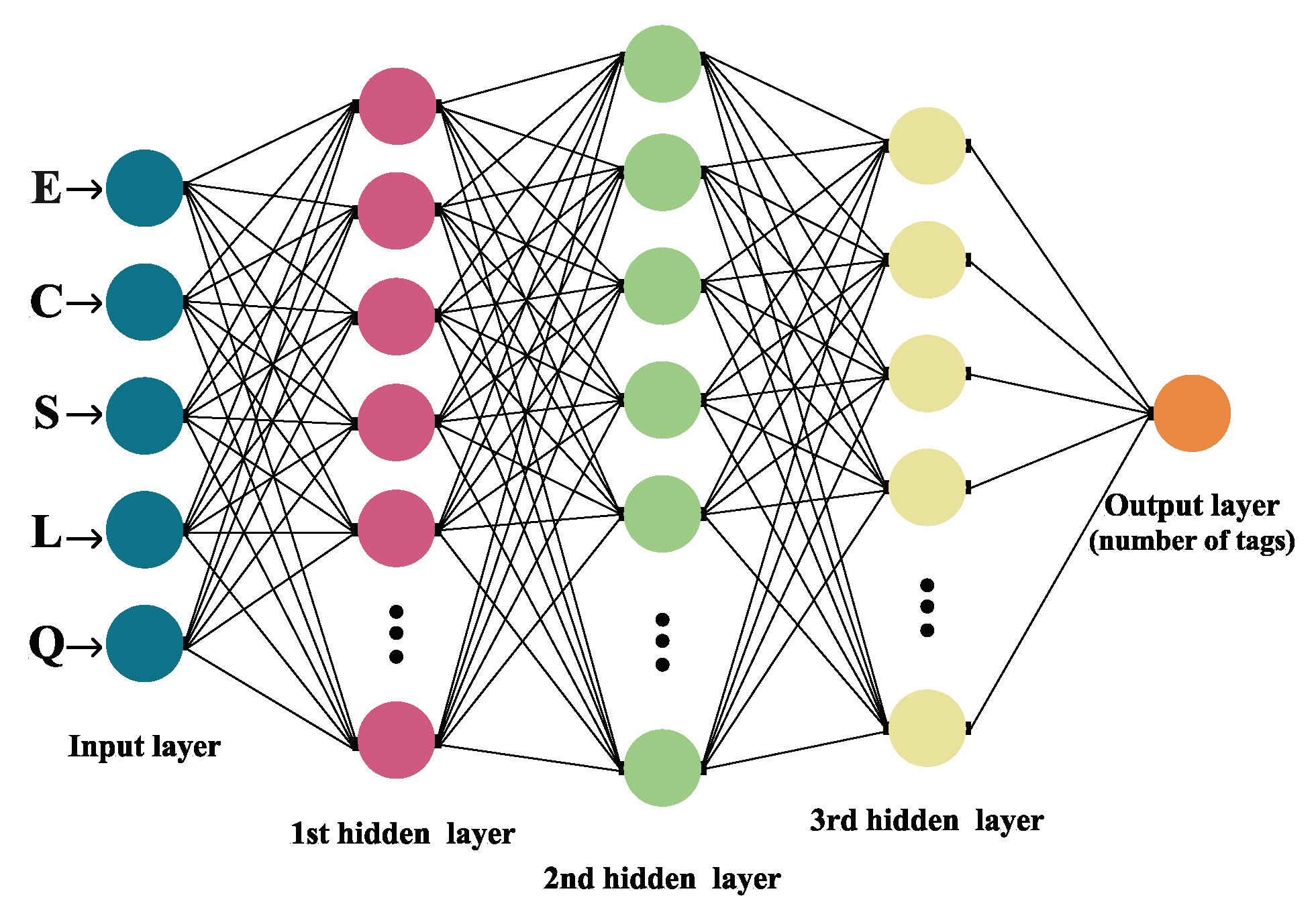
The architecture of the NN model displayed in this research is constructed of five layers, as depicted in
Figure 2. The first one is the input layer, followed by three hidden layers (one Dropout layer), and the final is the output layer. Applied activation functions were ReLU (in hidden layers) and Softmax (within the output layer). Data used for the input layer were number
Q, frame size
L and the number of
S successful,
E empty and
C collision slots. The number of tags that are associated with a particular distribution of slots within a frame is classified in the final exit layer.
The data were further partitioned in a ratio, with of the data used for training and the other for testing, with the target values being the number of tags, and all other values were provided as input. The training data were pre-processed and normalized, whereas target values were coded with One Hot Encoded with Keras library for better efficiency. By doing so, the integer values of the number of tags are encoded as binary vectors. The dropout rate (probability of setting outputs from the hidden layer to zero) was specified to be 20%. The number of neurons varies based on the frame size, ranging from 64 to 1024 for the first four layers.
Since the classification of the number of tags is a multi-class classification problem, for this research, the Categorical Cross-Entropy Loss function was applied as the loss (cost) function with several optimizer combinations. Another important aspect of the NN model architecture was thoroughly examined, and that is the selection of optimizers and learning rates. Optimizers attempt to help the model converge and minimize the loss or error function, whereas the learning rate decides how much the model needs to be altered in response to the estimated error every time the model weights are updated [
48]. Tested optimizers were Root Mean Square Propagation (RMSProp), Stochastic Gradient Descent (SGD) and Adaptive Moment Optimization (Adam). Adam provided the most accurate estimation results and was onward utilized in the learning process with 100 epochs and a 0.001 learning rate.
3.1.3. Random Forest Model
At the beginning of this century, L. Breiman proposed the Random Forest algorithm, an ensemble-supervised ML technique [
51]. Today, RF is established as a commonly utilized non-parametric method applied for both classification and regression problems by constructing prediction rules based on different types of predictor variables without making any prior assumption of the form of their correlation with the target variable [
52]. In general, the algorithm operates by combining a few arbitrary decision trees and onward aggregating their predictions by averaging. Random Forest has been proven to have exceptional behavior in scenarios where the amount of variables is far greater than the number of observations and can have good performance for large-scale problems [
53]. Studies have shown RF to be a very accurate classifier in different scenarios, it is easily adapted for various learning tasks, and one of its most recognizable features is its robustness to noise [
54]. That is why Random Forest has been used for numerous applications such as bioinformatics, chemoinformatics, 3D object recognition, traffic accident detection, intrusion detection systems, computer vision, image analysis, etc. [
11,
53].
A more formal definition of Random Forest is as follows. A Random Forest classifier is a collection made out of tree-structured classifiers, namely
, where
are independent random vectors that are identically distributed for an input
x, every tree will toss a unit vote for the most favored class [
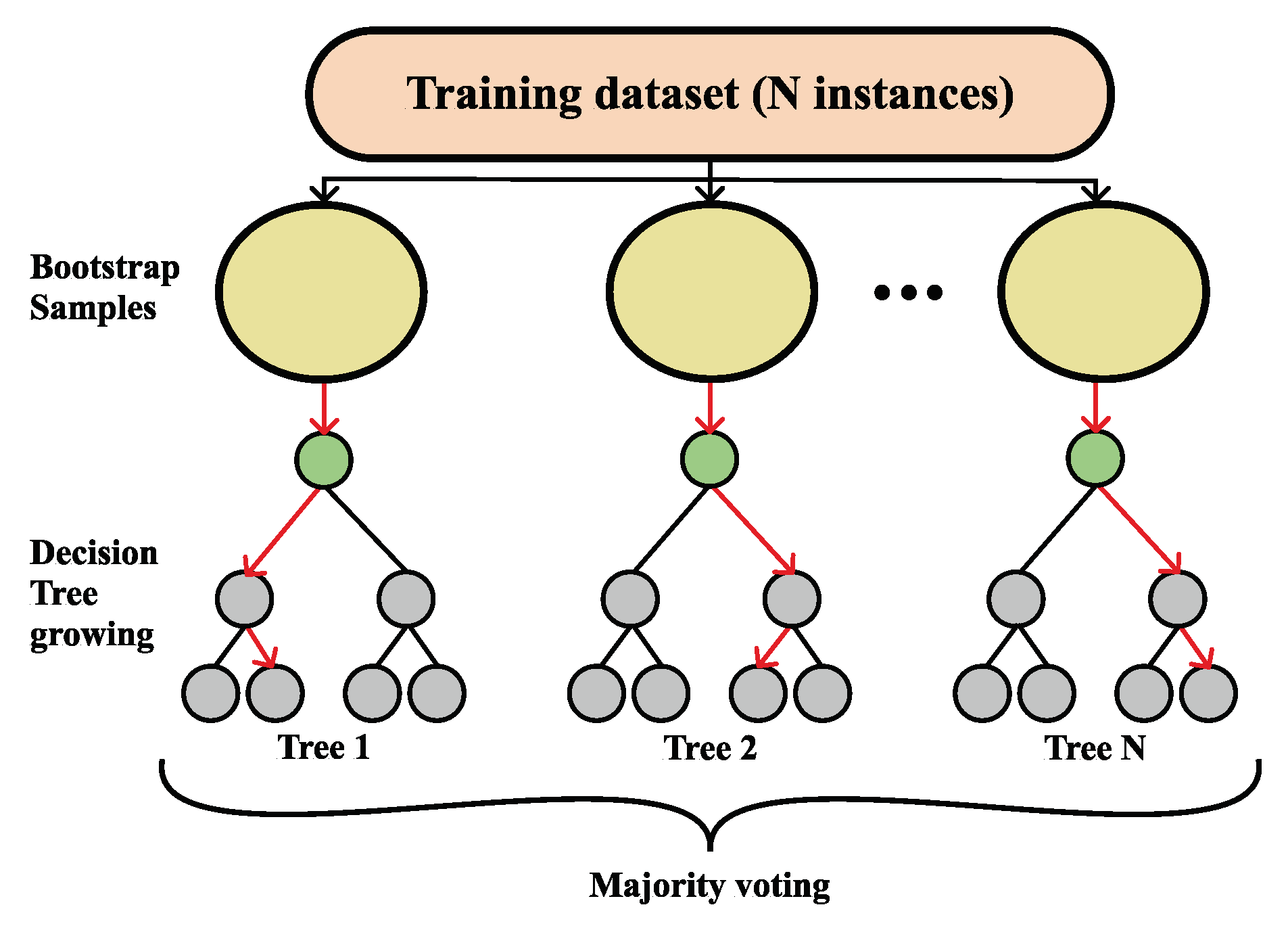
55], as shown in
Figure 3.
The bagging approach is used for producing the tree, i.e., by generating random slices of the training sets using substitution, which means that some slices can be selected more than once and others not at all [
56]. Given a particular training set
S, generated classifiers
toss a vote, thus making a
bagged predictor and, at the same time, for every pair
from the training set and for every
that did not contain
, votes from
are set aside as
out-of-the-bag classifiers [
51]. Commonly, a partition of samples is on the training set by taking two-thirds for tree training and leaving one-third for inner cross-validation, thus removing the need for cross-validation or a separate test set [
56]. The user is the one defining the number of trees and other hyper-parameters that the algorithm uses for independent tree creation performed without any pruning, where the key is to have a low bias and high variance, and the splitting of each node is based on a user-defined number of features that are randomly chosen [
52]. In the end, the final classification is obtained by majority vote, i.e., the instance is classified into the class having the most votes over all trees in the forest [
54].
Aiming to produce the best classification accuracy, in this research, hyper-parameter tuning has been performed by utilizing the GridSearchCV class from the scikit-learn library with five-fold cross-validation.
This is performed following the above reasoning for making a structure for each particular tree. By controlling the hyper-parameters, one can supervise the architecture and size of the forest (e.g., the number of trees (n_estimators)) along with the degree of randomness (e.g., max_features) [
52]. Therefore, for every frame size, the hyper-parameters presented in
Table 3 were tested, resulting in a separate RF model for each of the frame sizes, as presented in
Table 4.
