Enhanced Radio Map Interpolation Methods Based on Dimensionality Reduction and Clustering

Abstract

The received signal strength (RSS) based Wi-Fi fingerprinting method is one of the most potential and easily deployed approaches for a reliable indoor positioning system. However, due to the labor intensive and time-consuming radio map construction process, interpolation is often incorporated. To ensure the interpolated radio map is robust against environmental noise and RSS fluctuations, we propose two novel interpolation methods, termed as DimRed and DimRedClust, for an improved radio map construction. The former performs dimensionality reduction prior to the interpolation while the latter employs both the dimensionality reduction and clustering before interpolating the radio map. For dimensionality reduction, principal component analysis (PCA) or truncated singular value decomposition (TSVD) is adopted to profoundly extract essential features from the RSS data while the K-means algorithm is used to partition the reference points (RPs) into several clusters. Subsequently, the RSS for all virtual points are interpolated via inverse distance weighting (IDW). Numerical results based on the real-world multi-floor multi-building dataset confirm the supremacy of the proposed schemes over the baseline IDW interpolation. Compared to the baseline IDW, the proposed PCA-K-means-IDW, TSVD-K-means-IDW, PCA-IDW, and TSVD-IDW could attain a performance gain in terms of average positioning error of up to 30.17%, 30.93%, 19.33%, and 21.61%, respectively.

1. Introduction

In the recent years of this globalized era, the rapid evolution of wireless technology has led to the swift development of location-based services (LBS), which utilize the geographical location of a user to provide services or information accordingly. In light of the blooming of LBS, the demand for an accurate and real-time indoor positioning system (IPS) rises to fulfill the need for indoor LBS, which are popularly used in sectors, such as hospitals, indoor parking lots, airports, and shopping malls, for location identification and indoor navigation [1,2]. While current mature technology such as Global Positioning System (GPS), a type of global navigation satellite system (GNSS), is widely used for outdoor navigation and positioning, it is nevertheless not suitable for indoor localization purposes. This is due to the requirement for a direct line of sight (LOS) between the satellites and the user, which is almost impossible to be achieved in an indoor environment. Moreover, the signal is often weakened due to obstructions as it penetrates through the thick walls of a building, resulting in the accuracy of the indoor positioning information falling short of expectations [1,2,3].

In view of that, various wireless technologies are being considered and researched for their potential applications in indoor positioning. For instance, some of the available approaches include Bluetooth, radio frequency identification (RFID), ultra-wideband (UWB), geomagnetism, visible light and Wi-Fi [2,3]. In Wi-Fi based IPSs, the different localization schemes include the time of arrival (ToA), time difference of arrival (TDoA), angle of arrival (AoA) and the fingerprinting methods [2,3,4,5,6]. Nonetheless, it is worth mentioning that among the many existing technologies, the received signal strength (RSS) based Wi-Fi fingerprinting method has garnered the most attention since it does not require any additional hardware besides the readily available Wi-Fi access points (APs) and mobile devices with built-in network interface card (NIC) for RSS measurements [2,4]. This also implies that no extra cost would be incurred. Considering the fact that Wi-Fi networks have already been widely deployed and are capable of providing ubiquitous coverage, whereas mobile devices have long become part and parcel of our daily lives, it is thus safe to say that this technology is an infrastructure-less approach. However, since Wi-Fi networks are initially intended for wireless communication purposes and are not designed to support indoor positioning, the Wi-Fi signal is always prone to reflections, shadowing and multipath interference introduced by the obstacles (walls, doors, furniture and even human) present in an indoor environment [4]. Moreover, during RSS measurements, even the motion and the way the user carries the mobile device would affect the RSS values measured and thus affecting the positioning accuracy in indoor location prediction.

Generally, two phases are involved in the RSS-based Wi-Fi fingerprinting method, which are known as the offline and online phases. In the offline phase, a site survey must first be performed at the area of interest where the indoor localization will take place. As a result, a radio map, which contains the location labeled RSS measurements from surrounding APs at specific reference points (RPs), is constructed. Meanwhile, in the online phase, the RSS values measured from all the visible APs that can be detected from the user’s unknown location create a test sample which will then be compared with the RSS stored in the constructed radio map via a machine learning algorithm, thus predicting the user’s current location [2,3]. However, the radio map construction, which requires the RSS from surrounding APs to be collected at each of the RP would be labor-intensive and time-consuming. This issue is exacerbated under particular circumstances, such as having a large indoor environment of interest (multi-floor and multi-building), repeated sampling at each RP to obtain the average RSS vectors to be stored as fingerprints in the radio map so as to reduce the effect of outliers, and sampling in all four directions to take the impact of sheltering of the human body on RSS measurements into consideration, where all these would ultimately result in an increased workload [7]. In [7], principal component analysis (PCA) is adopted prior to location prediction with the aim to reduce the computational cost due to a large number of APs detected in a real-world scenario.

In light of the above, we propose two interpolation methods, i.e., DimRed, which is based on dimensionality reduction and DimRedClust, which is based on both dimensionality reduction and clustering as alternatives to a more enhanced radio map construction. PCA or truncated singular value decomposition (TSVD) is first adopted to extract key features from the sparse RSS data and to reconstruct it for a better feature representation. Besides eliminating redundancy while retaining maximal information, it also helps to reduce the impact of noise and outliers on the high dimensionality radio map. Subsequently, the K-means algorithm is used to partition the RPs into several clusters with the assumption that RPs closer to each other will demonstrate similar RSS attributes. Next, the interpolation of RSS for all virtual points (VPs) are performed for each cluster via inverse distance weighting (IDW) interpolation. Lastly, the interpolated radio map is combined with the initial radio map to form a new radio map which will be used for indoor localization via the K Nearest Neighbor (KNN) algorithm.

To the best of our knowledge, no prior work attempts to enhance the quality of the radio map and localization performance by performing dimensionality reduction or employing both the dimensionality reduction and clustering before radio map interpolation. In summary, the main contributions of this work are outlined as follows:

• Two novel interpolation techniques, i.e., DimRed and DimRedClust, are proposed to effectively enhance the robustness of the interpolated radio map against the environmental noise and RSS fluctuations and to reduce the storage requirement and computational cost.
• Two DimRed methods, abbreviated as PCA-IDW and TSVD-IDW, are developed. To profoundly extract the key features with maximal information from the RSS data, the former adopts PCA prior to the IDW interpolation while the latter employs TSVD before performing IDW on the radio map.
• Two DimRedClust approaches, which are known as PCA-K-means-IDW and TSVD-K-means-IDW, are developed. Both the PCA-K-means-IDW and TSVD-K-means-IDW methods utilize IDW interpolation. Still, in order to confine the selection of nearest neighbors to only the known RPs located in the same cluster, the former performs K-means clustering on the low-dimensional principal component-based fingerprint matrix. At the same time, the latter applies K-means clustering after TSVD is executed.
• A comprehensive investigation is carried out to assess and analyze the performance of all the proposed techniques viz a viz the IDW scheme in terms of the average positioning error, root mean square error (RMSE) of the easting, northing, and positioning error. Besides that, various essential statistics of the positioning error are characterized, and the effects of hyperparameters are also analyzed in detail.

The remainder of this paper is organized as follows: Section 2 presents a review of recent literature on radio map interpolation, while Section 3 contains the description of the IDW interpolation method used as a benchmark in this paper. Meanwhile, Section 4 further elaborates on the proposed methods for interpolation, including brief descriptions of the PCA, TSVD, and K-means algorithms. Thereafter, the performance evaluation and discussion of findings are presented in Section 5 followed by a conclusion of this paper in Section 6.

2. Related Works

Numerous techniques are proposed to overcome the problem caused by the time consuming and labor-intensive radio map construction. Kiring et al. investigated the effect of spatial correlation (spatial patterns related to the geographical distributions of signals) in the densely collected RSS measurements. This spatial correlation which exists due to the proximity distance between the RPs is exploited for accurate prediction of the user’s unknown location. To interpolate the RSS values for the incomplete radio map, the IDW and KNN algorithms are used, and their performance is compared with each other. The interpolation errors computed from the RMSE between the predicted and actual RSS measurements for both the IDW and KNN algorithms are analyzed with and without the spatial correlation over a variety of sparsity parameters [8].

Another approach is to calculate the RSS fingerprints via linear and Delaunay interpolations for radio map creation. The calculated RSS values for the interpolation points are compared with the actual RSS measurements collected beforehand, thus producing the interpolation errors. Subsequently, the performance of the two interpolation techniques is also compared among each other [9].

In [10], a graph-based signal interpolation that treats the RSS measurements as signals defined over a graph consisting of nodes representing different physical locations and weighted edges denoting the distances between locations is presented. Such a graph-based interpolation method captures global information and predicts the RSS of all unknown nodes based on the relationships among the known nodes, apart from the relationships between known and unknown nodes. Comparisons are also made among various graph construction strategies, and from the simulation results, it is found that the graph-based signal interpolation could outperform the conventional interpolation methods, which are IDW, radial basis function (RBF), and model-based interpolation (MBI).

Moreover, Zuo et al. presented another Kriging based interpolation method which relies on the spatial distribution correlation of the RSS to create a radio map covering the entire experiment testbed, including those inaccessible regions where RSS measurements would be hindered. This method is capable of achieving a positioning error of less than 3 m in most of the conditions investigated [11].

Besides, an interesting image-driven approach which treats the radio propagation data as an image and estimates the spatial distribution of the RSS via image processing techniques is adopted in [12]. The proposed deep learning (DL) framework transforms the spatial interpolation problem into a shadowing adjustment problem via the path loss regression and employs the neural network (NN) structure for the shadowing adjustment problem. A gradual training method is also used, which trains the encoding/decoding block separately for the stability of the NN structure. The DL framework indeed outperformed other existing image-driven DL methods, such as a generative adversarial network (GAN)-based model and spatial interpolation with convolutional neural networks (CNN).

Zhao et al. used the universal Kriging (UK) interpolation method to calculate the RSS values for the defined interpolation points besides virtually augmenting the space boundary. Such augmentation is done by defining extra interpolation points outside of the original space in order to overcome the boundary effect, which reduces the localization accuracy at the boundary. Even with only 28 known RPs (the RSS values for the remaining 84 VPs are interpolated), this technique is still capable of achieving an average positioning error that is comparable to that of when 112 known RPs are collected [13].

To reduce the workload during site surveying for the construction of a radio map, Ye et al. developed a crowdsourcing approach instead for radio map generation using the crowdsourced samples in [14]. However, this crowdsourcing approach, which is random and voluntary, gives rise to a non-uniform spatial distribution problem that exists when certain grids of the experimented indoor environment contain too few or lack crowdsourced samples. To overcome this problem, a binary polynomial function is adopted to interpolate more RSS fingerprints for the grid with insufficient crowdsourced samples based on the RSS fingerprints of its neighboring grids. In this case, only sufficient grid distinct fingerprints are used for interpolation instead of considering as many surrounding grids as possible since the inclusion of faraway grids might cause larger RSS deviations and thus affect the quality of the interpolated radio map.

Wang et al. designed an improved low-rank matrix completion method for a more rapid radio map construction. Assuming that the RSS data matrix in the radio map has low-rank characteristics, the radio map construction can then be modeled as a low-rank matrix completion problem (completion of an incomplete matrix into a complete matrix). In view of that, it is possible to collect RSS values at only a small number of RPs and to further fill up the RSS values in the radio map in order to convert it into a complete Wi-Fi fingerprinting database using the low-rank matrix completion algorithm with the Frobenius parameter (F-parameter) integrated into it for the stability of the model solution when filling up the data. Apart from that, the low-rank matrix recovery algorithm is also used to suppress noise caused by the environment and equipment [15].

A least absolute shrinkage and selection operator (LASSO) based interpolation scheme is proposed in [16], which enabled the reconstruction of a radio map by RSS fingerprints interpolation at a finer granularity based on the RSS fingerprints collected for the RPs at a coarser granularity. The sparse reconstruction of the radio map using the sparse recovery algorithm is made possible due to the extremely sparse feature of the RSS fingerprints. An outlier detection scheme is also introduced into the radio map interpolation procedure to reduce the effect of outliers present during the offline phase and ensure that the interpolation is performed using the RSS values of RPs that are free of outliers.

Talvitie et al. on the other hand, investigated the performance of various interpolation and extrapolation methods, including linear interpolation, minimum method extrapolation, mean method extrapolation, gradient method extrapolation, nearest neighbor and IDW that are used to construct a complete radio map. Comparisons are made between the estimated RSS fingerprints and the actual RSS fingerprints while varying the percentages of the interpolated RSS fingerprints. This is done in order to determine the average RSS estimation error of the different interpolation and extrapolation methods. The performance of four cases, including the original fingerprint, the partial fingerprint (the incomplete fingerprint without any interpolation), the interpolated fingerprint, and the combined interpolated and extrapolated fingerprint, are also compared in their resulting indoor positioning accuracy [17].

In [18], Jan et al. applied the Kriging algorithm to calculate the RSS values at more unobserved locations, thus creating an extended database apart from the RSS fingerprints measured at a small number of RPs. By varying the size of the extended database, i.e., the number of basic RPs and Kriging RPs, its effect on the positioning error is evaluated apart from comparing the interpolated database to the measured database to identify the RSS interpolation error.

Similar work is also presented in [19], where different interpolation functions such as Euclidean distance linear basis, multi-quadratic, thin-plate spline and polyharmonic spline functions are used to calculate the RSS values for the interpolated points. Besides, the impacts of density and distribution of the known RPs on the indoor localization error are also investigated simultaneously. An assumption made here is that the radio frequency (RF) signals for locations nearer to the beacons tend to have a better quality than that of locations further away. Thus, the zones nearer to the beacons are assigned with a lower density of known RPs, whereas the zones further away from the beacons are assigned with a higher density of known RPs instead.

Meanwhile, Bi et al. proposed an adaptive path loss model interpolation method that first performs crowdsourcing to collect RSS fingerprints at sparse RPs followed by establishing path loss models for all visible APs with the help of several RPs in a small area. The least-squares method is then used to estimate the optimal parameters for the path loss models. Afterwards, the RSS values of the interpolation points could be calculated based on the path loss models. A performance comparison is also made among their proposed method with the IDW and Kriging interpolation approaches. However, this method requires knowledge of the exact locations of the APs [20].

Furthermore, another radio map construction method based on crowdsourcing and interpolation is also proposed by Bi et al. The RSS fingerprints are collected at a small number of specified RPs via crowdsourcing with the usage of different devices followed by normalization account for the device heterogeneity issue. The process is then carried on with the IDW interpolation of RSS values at different interpolated points. After the radio map interpolation, PCA is then used for dimensionality reduction of the new radio map formed from the combination of the initial and interpolated radio map to reduce the computational cost [7].

On the other hand, Boujnah et al. also proposed a method for localization based on crowdsourcing, data clustering and multidimensional interpolation. The collected data via crowdsourcing are partitioned into small areas according to the cell identifiers of the received signals. Their corresponding RSS fingerprints will only be clustered via K-means or fuzzy C-means if the cardinality of the partition exceeds a fixed threshold. Subsequently, RBF with Gaussian kernel is adopted to identify the interpolation function assigned to each cluster to estimate the user’s unknown location per cluster [21].

3. Radio Map Interpolation

In this section, the construction of initial radio map and the existing IDW interpolation method are explained. Throughout the paper, scalars, vectors, and matrices are denoted as non-bold variables (e.g., x), lower-case bold variables (e.g., x), and upper-case bold variables (e.g., X), respectively. The transpose operation is represented by superscript T.

3.1. Construction of Initial Radio Map

Consider an indoor localization system with D APs and M predefined RPs. In the offline phase, the RSS fingerprints, i.e., the RSS readings measured from all the APs, for each of the RPs are collected. Then, the radio map $\mathit{\chi }$, can be obtained by concatenating the location coordinates with their corresponding RSS fingerprints. Mathematically, $\mathit{\chi }$ can be formulated as

$$\mathit{\chi }=\left[\begin{array}{cc}\left(\begin{array}{cccc}{l}_{1,1}& l_{1,2}& \cdots & l_{1,Q}\end{array}\right)& \left(\begin{array}{cccc}{r}_{1,1}& r_{1,2}& \cdots & r_{1,D}\end{array}\right)\\ ⋮& ⋮\\ \left(\begin{array}{cccc}{l}_{m,1}& l_{m,2}& \cdots & l_{m,Q}\end{array}\right)& \left(\begin{array}{cccc}{r}_{m,1}& r_{m,2}& \cdots & r_{m,D}\end{array}\right)\\ ⋮& ⋮\\ \left(\begin{array}{cccc}{l}_{M,1}& l_{M,2}& \cdots & l_{M,Q}\end{array}\right)& \left(\begin{array}{cccc}{r}_{M,1}& r_{M,2}& \cdots & r_{M,D}\end{array}\right)\end{array}\right]$$

(1)

where $\mathit{\chi }\in {ℝ}^{M\times \left(Q+D\right)}$, ${\mathit{l}}_m={\left[\begin{array}{cccc}{l}_{m,1}& l_{m,2}& \cdots & l_{m,Q}\end{array}\right]}^T$ denotes the location identifier vector for RP m, Q is the total number of location identifiers used to specify each RP, ${\mathit{r}}_m={\left[\begin{array}{cccc}{r}_{m,1}& r_{m,2}& \cdots & r_{m,D}\end{array}\right]}^T$ represents the RSS fingerprint vector at RP m, $r_{m,d}$ signifies the RSS from AP d at RP m, $m\in \left[1,M\right]$ and $d\in \left[1,D\right]$. (1) can also be re-written more compactly as follows:

$$\chi =\left[\begin{array}{cc}\mathit{L}& \mathit{R}\end{array}\right]$$

(2)

where $\mathit{L}={\left[\begin{array}{cccc}{\mathit{l}}_1& {\mathit{l}}_2& \cdots & {\mathit{l}}_M\end{array}\right]}^T\in {ℝ}^{M\times Q}$ and $\mathit{R}={\left[\begin{array}{cccc}{\mathit{r}}_1& {\mathit{r}}_2& \cdots & {\mathit{r}}_M\end{array}\right]}^T\in {ℝ}^{M\times D}$.

In the online phase, the RSS vector at the unknown location u ${\mathit{r}}_u={\left[\begin{array}{cccc}{r}_{u,1}& r_{u,2}& \cdots & r_{u,D}\end{array}\right]}^T$ will be measured, and the user’s location can then be predicted by matching ${\mathit{r}}_u$ with the RSS data in the radio map via machine learning techniques. As such, the quality of the radio map plays a crucial role in dictating the localization performance. Generally, the localization performance tends to improve as the density of the RPs increases. Unfortunately, the fingerprint collection process is labor intensive and time consuming. In practice, various environmental disturbances and interferences could reduce the discernibility of the fingerprints between RPs, thereby leading to false fingerprint matching. Thus, to ensure reliable localization, it is imperative to establish an enhanced interpolated radio map that is robust against the environmental disturbances and interferences.

3.2. Virtual Points Generation Using IDW Interpolation

IDW interpolation is a deterministic spatial interpolation approach that estimates an unknown value at a location with the aid of some known values from its surrounding with corresponding weights. More specifically, the RSS values from the d-th AP at the u-th VP which is denoted by $r_{u,d}$ could be computed based on the RSS of its surrounding N nearest known RPs via (3) as follows:

$$r_{u,d}=\frac{{\displaystyle \sum _{i=1}^N{w}_i{\tilde{r}}_{i,d}}}{{\displaystyle \sum _{i=1}^N{w}_i}}$$

(3)

where u denotes the index of the VPs, i refers to the index of the N nearest known RPs, ${\tilde{r}}_{i,d}$ is the RSS of the d-th AP at i-th nearest known RPs that is chosen from the d-th column of $\mathit{R}$, and $w_i$ signifies the interpolation weight. Mathematically, $w_i$ can be expressed as

$$w_i=\frac{1}{d_{(u,i)}{}^{\alpha }}$$

(4)

where $d_{\left(u,i\right)}$ stands for the Euclidean distance between the u-th VP and the i-th nearest known RP, while α indicates the power parameter which determines the rate at which the weight decreases with the increase in distance. As α increases, the weights decrease more rapidly for distant points. Thus, for an extremely high α, only the immediate surrounding RPs will influence the interpolation of RSS for the VP. When $\alpha =2$, it is commonly known as the inverse distance squared weighted interpolation.

An assumption made in the IDW interpolation is that the values of points closer to each other tend to be more similar than those located further away. Hence, the values of those points nearer to the interpolation location will generally have more influence on the predicted value than those further away. As such, the points nearest to the interpolation location will be assigned with greater weights that diminish as a function of distance.

4. Proposed Methods

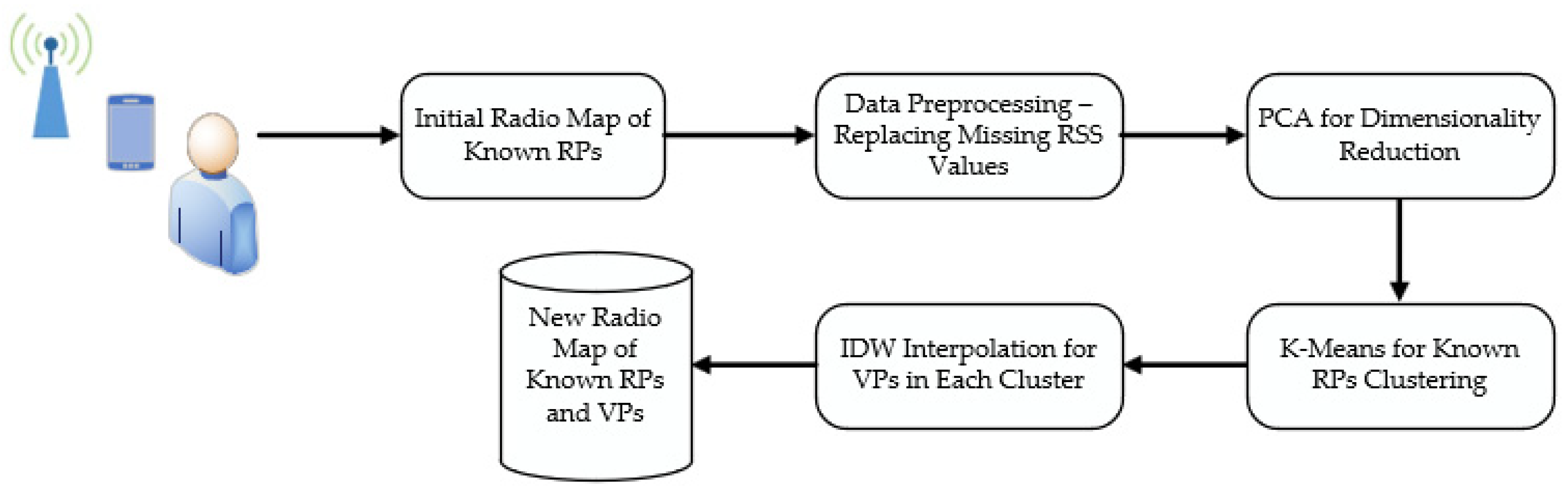
Two radio map interpolation schemes are proposed for an enhanced radio map construction. The DimRed interpolation scheme involves two main steps which are dimensionality reduction and VP interpolation while the DimRedClust interpolation scheme encompasses three main steps which include dimensionality reduction, clustering and VP interpolation. In other words, the only difference between the two proposed interpolation schemes is the addition of the clustering process in between. The block diagram for the DimRedClust interpolation scheme is as depicted in Figure 1 below. The DimRed interpolation scheme also follows a similar flow except for the clustering process being skipped.

Data preprocessing is first performed to the initial radio map to ensure that there are no missing values since it is common for some APs to be undetectable at faraway RPs. After data preprocessing has completed, dimensionality reduction is performed on the initial high-dimensional fingerprint matrix $\mathit{R}$ using PCA or TSVD in order to reduce the large number of features present in the radio map to P principal components by removing redundant information while preserving as much useful information as possible. As a result, only the key features are extracted and $\mathit{R}$ will be transformed to a low-dimensional principal component-based fingerprint matrix $\mathit{H}\in {ℝ}^{M\times P}$. By reducing the dimension of the Wi-Fi fingerprint, apart from reducing the computational cost, the influence of noise and outliers initially present in $\mathit{R}$ will also be mitigated, which in turn improves the performance during location prediction.

Next, all the known RPs are partitioned into C clusters based on their eastings and northings using K-means algorithm, as the known RPs located nearer to each other will tend to have similar RSS characteristics as compared to known RPs that are located further away. After grouping the known RPs into clusters, the process is then followed by cluster matching of the VPs. More explicitly, a cluster whose centroid has the shortest distance to the VP will be selected as the delegate cluster for that VP. Note that this step is only performed for the DimRedClust interpolation scheme and not for the DimRed interpolation scheme.

IDW interpolation is carried out for the VPs in each cluster. This implies that the RSS of the VPs will only be interpolated based on the known RPs located in the same cluster. This prevents the occurrence of a situation whereby one of the nearest neighbors of the VP is actually located rather far apart from that VP, and thus considering that nearest neighbor during interpolation might have resulted in an adverse effect.

Finally, a new radio map is obtained by combining the initial radio map, which contains the RSS for the known RPs and the interpolated radio map, which contains the RSS for the VPs. The reason for combining both the initial and interpolated radio maps to form the new radio map is to increase the density of the RPs as the indoor localization performance generally improves when the density of RPs distributed across the indoor environment increases. This new radio map is then used for the indoor location prediction of the testing samples via the KNN algorithm and its corresponding performance is evaluated.

In the following, the working principles of PCA, TSVD, and K-means used in the proposed interpolation methods will be presented.

4.1. Dimensionality Reduction of Radio Map Using PCA

PCA is a well-known dimensionality reduction method which transforms a large set of variables into smaller ones while still preserving most of the information. This could be achieved by extracting only the essential features and creating linearly uncorrelated variables called principal components. Generally, most of the information within the initial variables would be placed in the first principal component (to achieve the largest possible variance), thus allowing for dimensionality reduction by discarding those principal components with low information. The principal components show the directions of the data that explain a maximal amount of variance. The larger the variance, the larger the dispersion of data points along the line, thus the more information it contains.

A covariance matrix $\mathit{B}$, is a symmetric matrix with both its rows and columns having the same size as the number of dimensions/variables of the dataset, i.e., the number of APs D of the radio map $\mathit{\chi }$ in the context of indoor positioning. Its entries consist of covariances associated with all possible pairs of initial variables, while the diagonal denotes the variance of each initial variable. Note that this covariance matrix must be computed to identify the correlations between the variables of the dataset. In the context of indoor positioning, the correlation between two APs of the radio map cov(x, y) can be computed as shown in (5), where M is the number of RPs/instances in the radio map, $x_i$ and $y_i$ denote the RSS from AP x and y at RP i, respectively, while $\overline{x}$ and $\overline{y}$ are the sample means of AP x and y, respectively. If the covariance is positive, this implies that the two variables are correlated, while a negative covariance suggests that the two variables are inversely correlated.

$$cov(\mathit{x},\mathit{y})=\frac{{\displaystyle \sum _{i=1}^M(x_i-\overline{x})(y_i-\overline{y})}}{M}$$

(5)

From the covariance matrix $\mathit{B}$, the eigenvectors $\mathit{v}$ and eigenvalues $\lambda$ are then computed to determine the principal components. Let the covariance matrix $\mathit{B}$, eigenvectors $\mathit{v}$ and eigenvalues $\lambda$ be a square matrix, a vector and a scalar that satisfies (6):

$$\mathit{B}\mathit{v}=\lambda \mathit{v}$$

(6)

The eigenvalues $\lambda$ of $\mathit{B}$ are the roots of the characteristic equation and can be calculated as defined in (7) where $\mathit{I}$ is an identity matrix:

$$\det (\lambda \mathit{I}-\mathit{B})=0$$

(7)

Subsequently, for each $\lambda$, the basic eigenvectors could be obtained by identifying the basic solutions to (8):

$$(\lambda \mathit{I}-\mathit{B})\mathit{v}=0$$

(8)

The eigenvectors of the covariance matrix are the directions of the axes where the variance is the largest (principal components) while the eigenvalues are the coefficients which tell about the variance in each principal component. Hence, the principal components could be ranked according to their significance by ranking the eigenvectors in the order of their eigenvalues.

By discarding those principal components of lower eigenvalues, the remaining P principal components will be used to form a matrix called a feature vector $\mathit{F}$, as shown in (9), whose columns consist of the eigenvectors $\mathit{v}$ of the principal components that are not removed.

$$\mathit{F}=\left[\begin{array}{cccc}{v}_{1,1}& v_{1,2}& \cdots & v_{1,P}\\ v_{2,1}& v_{2,2}& \cdots & v_{2,P}\\ ⋮& ⋮& ⋮& ⋮\\ v_{D,1}& v_{D,2}& \cdots & v_{D,P}\end{array}\right]$$

(9)

Finally, the data are reoriented from the original axes to those represented by the principal components via multiplication of the high-dimensional fingerprint matrix $\mathit{R}$ by the feature vector $\mathit{F}$ and the output of the PCA is a low-dimensional fingerprint matrix $\mathit{H}$ which can be written as

$$\mathit{H}=\left[\begin{array}{cccc}{h}_{1,1}& h_{1,2}& \cdots & h_{1,P}\\ h_{2,1}& h_{2,2}& \cdots & h_{2,P}\\ ⋮& ⋮& ⋮& ⋮\\ h_{M,1}& h_{M,2}& \cdots & h_{M,P}\end{array}\right]$$

(10)

where $p=\left[1, 2, \cdots , P\right]$.

For the proposed DimRed interpolation technique, IDW will then be performed on the low-dimensional fingerprint matrix $\mathit{H}$ as follows:

$$r_{u,p}=\frac{{\displaystyle \sum _{i=1}^N{w}_i{\tilde{h}}_{i,p}}}{{\displaystyle \sum _{i=1}^N{w}_i}}$$

(11)

where ${\tilde{h}}_{i,p}$ is the value of the p-th principle component for the i-th nearest known RPs. More explicitly, the N nearest neighbors for the p-th principle component are selected from the p-th column of $\mathit{H}$ based on the Euclidean distance.

4.2. Dimensionality Reduction of Radio Map Using TSVD

SVD is a matrix decomposition technique that reduces a matrix into its constituent elements for a more simplified matrix calculation. In the context of indoor positioning, it involves the factorization of an $M\times D$ high-dimensional fingerprint matrix $\mathit{R}$ into a product of an $M\times M$ unitary matrix $\mathit{U}$, an $M\times D$ rectangular diagonal matrix $\mathit{S}$, and an $D\times D$ complex unitary matrix ${\mathit{V}}^T$ as shown in (12).

$$\mathit{R}=\mathit{U}\mathit{S}{\mathit{V}}^T$$

(12)

The diagonal of the S matrix contains the singular values of the fingerprint matrix $\mathit{R}$ which has a form as shown in (13) where ${\sigma }_1\ge {\sigma }_2\ge \dots \ge {\sigma }_r\ge 0$ are the singular values of the fingerprint matrix $\mathit{R}$ with rank r arranged in weakly decreasing order. Note that every S matrix will have a singular value decomposition. Meanwhile, the columns of the U matrix are the left singular vectors of fingerprint matrix $\mathit{R}$ while the columns of the V matrix are the right singular vectors of fingerprint matrix $\mathit{R}$.

$$\mathit{S}=\left(\begin{array}{ccc}{\sigma }_1& & \\ & \ddots & \\ & & {\sigma }_r\end{array}\right)$$

(13)

TSVD belongs to one of the types of SVD method for dimensionality reduction, which works by setting all except the top few largest singular values in the S matrix to zero and using only the first few columns of U and V. It is often performed on the fingerprint matrix whereas PCA is performed on the covariance matrix instead. TSVD factorizes the fingerprint matrix such that the number of columns is equal to the truncation. The digits after the decimal place are dropped in order to mathematically shorten the value of float digits. For a given high-dimensional fingerprint matrix $\mathit{R}$, the TSVD will produce low-dimensional fingerprint matrix $\mathit{H}$ with the specified number of columns by retaining only P features as specified. In comparison with PCA, which is another similar technique, TSVD works better with sparse data which contains many zero values since it does not centre the data before computing the SVD. Similar to the DimRed interpolation technique that utilizes PCA, the interpolated principle component-based fingerprint matrix for DimRed with TSVD could be obtained by executing Equations (10) and (11).

4.3. Clustering of Reference Points Using K-Means

K-means is a simple yet powerful algorithm popularly used for clustering. In the context of indoor positioning, it attempts to group M RPs/instances in the radio map into C clusters based on the similarity in features shared by them. It is a centroid based algorithm that calculates the distances in order to assign an RP to a cluster and aims to minimize the sum of squared distances between the RPs in each cluster with their respective centroid as defined by the objective function J in (14), where $x_i$ denotes the coordinates for one of the M RPs while ${\mu }_j$ denotes the centroid for one of the C clusters.

$$J={\displaystyle \sum _{j=1}^C{\displaystyle \sum _{i=1}^M\left|\right|x_i-{\mu }_j|{|}^2}}$$

(14)

The algorithm involves a few steps which are briefly described as follows:

• Choose the number of clusters, C;
• Initialize C points as centroids, $\mu$ for each cluster as expressed in (15);

$$\mu ={\mu }_1,{\mu }_2,\dots {\mu }_C$$

(15)

3.

Assign each of the RP $x_i$ to the closest cluster centroid ${\mu }_j$ with the shortest Euclidean distance via (16);

$$\arg \underset{{\mu }_j\in \mu }{\min } dist{(x_i,{\mu }_j)}^2$$

(16)

4.

Re-compute the centroid ${\mu }_j$ according to the average of the newly formed cluster as shown in (17) where G denotes the set of RPs assigned to the j-th cluster;

$${\mu }_j=\frac{1}{G}{\displaystyle \sum _{i=1}^G{x}_i}$$

(17)

5.

Repeat Steps 3 and 4 until either one of the termination criteria is met, which could be either the centroids of the newly formed clusters no longer change, or all the RPs remain in the same cluster or the maximum number of iterations had reached.

Once the clusters are formed, the principal component based radio map will be split into C principal component based sub-radio maps ${\xi }_c\in {ℝ}^{G_c\times \left(Q+P\right)}$ according to the grouping of RPs obtained via K-means, where $c=\left[1, 2, \cdots , C\right]$, $G_c$ denotes the total number of RPs that are associated with cluster c, and ${\displaystyle \sum _{c=1}^C{G}_c=M}$. Since K-means is a hard clustering scheme, the sub-radio maps created will be mutually exclusive, i.e., each RP only belongs to one of the clusters. For the proposed DimRedClust technique, cluster matching will then be performed on the VP and IDW interpolation will be applied on the principal component based sub-radio map that corresponds to the cluster that the VP belongs to.

5. Results and Analysis

In this section, we perform a comparative performance study between the proposed schemes and the baseline IDW.

5.1. Experimental Setup

In this work, the publicly available UJIIndoorLoc dataset collected at University Jaume I is used to evaluate the performance of the proposed techniques and benchmark with those of the existing schemes. The dataset was collected across 3 buildings with either 4 or 5 floors, and this covered a total surface area of 108,730 m². Altogether, 520 wireless APs (WAPs) were adopted in the three buildings, which made up the 520 attributes of RSS values among the 529 attributes present in the dataset, alongside some other important attributes, such as Building ID, Floor ID, Easting, and Northing. A total of 21,049 samples were captured in the dataset, with 19,937 as training samples while the remaining 1111 as testing samples. The training samples include a total of 933 distinct RPs distributed across the 3 buildings [22].

Table 1. Number of RPs at each floor of each building.

Building	Floor	Number of RPs
0	0	54
	1	67
	2	70
	3	68
1	0	76
	1	60
	2	79
	3	50
2	0	67
	1	89
	2	73
	3	113
	4	67

shows the number of RPs available at each floor of each building.

Prior to dimensionality reduction and clustering, a data preprocessing step is first performed to the sparse UJIIndoorLoc dataset. This data sparsity exists due to the obstruction of certain out-of-range WAPs, as not all the 520 WAPs are detectable at each of the RPs. In the initial dataset, the default RSS values for undetectable WAPs are represented as +100 dBm. In general, a smaller RSS value implies a weaker signal, thus representing the RSS for missing WAPs with a large value such as +100 dBm might create confusion to the regressor for location prediction. Thus, a common practice is to represent missing RSS values for the weak APs with a value slightly smaller than the smallest detectable RSS. Since the weakest RSS present in the dataset is found to be −104 dBm, the suitable value that should be used to replace the RSS for missing WAPs is chosen to be −110 dBm [23].

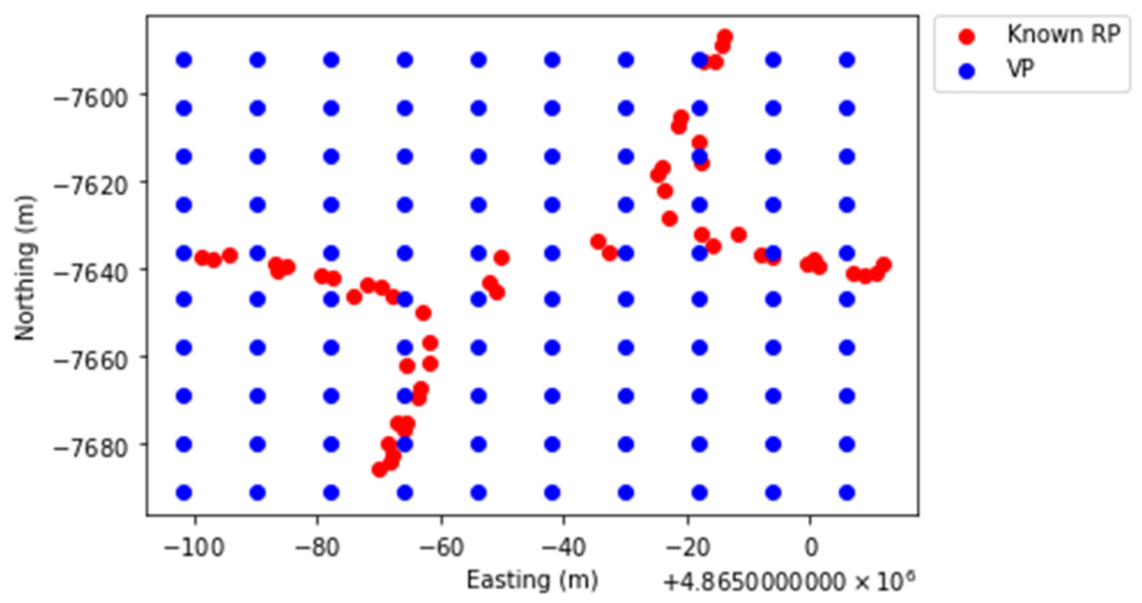
For the experimental purposes of the proposed interpolation methods, all the 933 RPs found in the training samples are treated as known RPs for the interpolation of RSS of the VPs. At each floor of each building, there are a total of 100 VPs (10 $\times$ 10) uniformly distributed across the area of interest. Figure 2 portrays an example of the distributions of known RPs and VPs for Building 0 Floor 0.

To evaluate the performance of the interpolated radio map in estimating the user’s location using machine learning technique, two metrics are used, i.e., RMSE and the average positioning error a. More explicitly, the RMSE is the standard deviation of the errors between the predicted values $\widehat{l_i}=[\widehat{l_1},\widehat{l_2},\dots ,\widehat{l_M}]$ given by the regression model and the actual values $l_i=[l_1,l_2,\dots ,l_M]$ from the dataset, where M is the total number of RPs/instances in the radio map and l can represent either the easting or the northing. The smaller the RMSE is, the better the regression model is able to fit the dataset. Mathematically, the RMSE for the easting and northing of each scenario can be expressed as follows:

$$RMSE=\sqrt{\frac{{\displaystyle \sum _{i=1}^M{(\widehat{l_i}-l_i)}^2}}{M}}$$

(18)

As for the average positioning error a, it is calculated based on the Euclidean distance between the predicted coordinates $(\widehat{x_i},\widehat{y_i})=[(\widehat{x_1},\widehat{y_1}),(\widehat{x_2},\widehat{y_2}),\dots ,(\widehat{x_M},\widehat{y_M})]$ and the actual coordinates $(x_i,y_i)=[(x_1,y_1),(x_2,y_2),\dots ,(x_M,y_M)]$ as given in Equation (19).

$$a=\frac{{\displaystyle \sum _{i=1}^M\sqrt{{(\widehat{x_i}-x_i)}^2+{(\widehat{y_i}-y_i)}^2}}}{M}$$

(19)

5.2. Localization Performance Evaluation

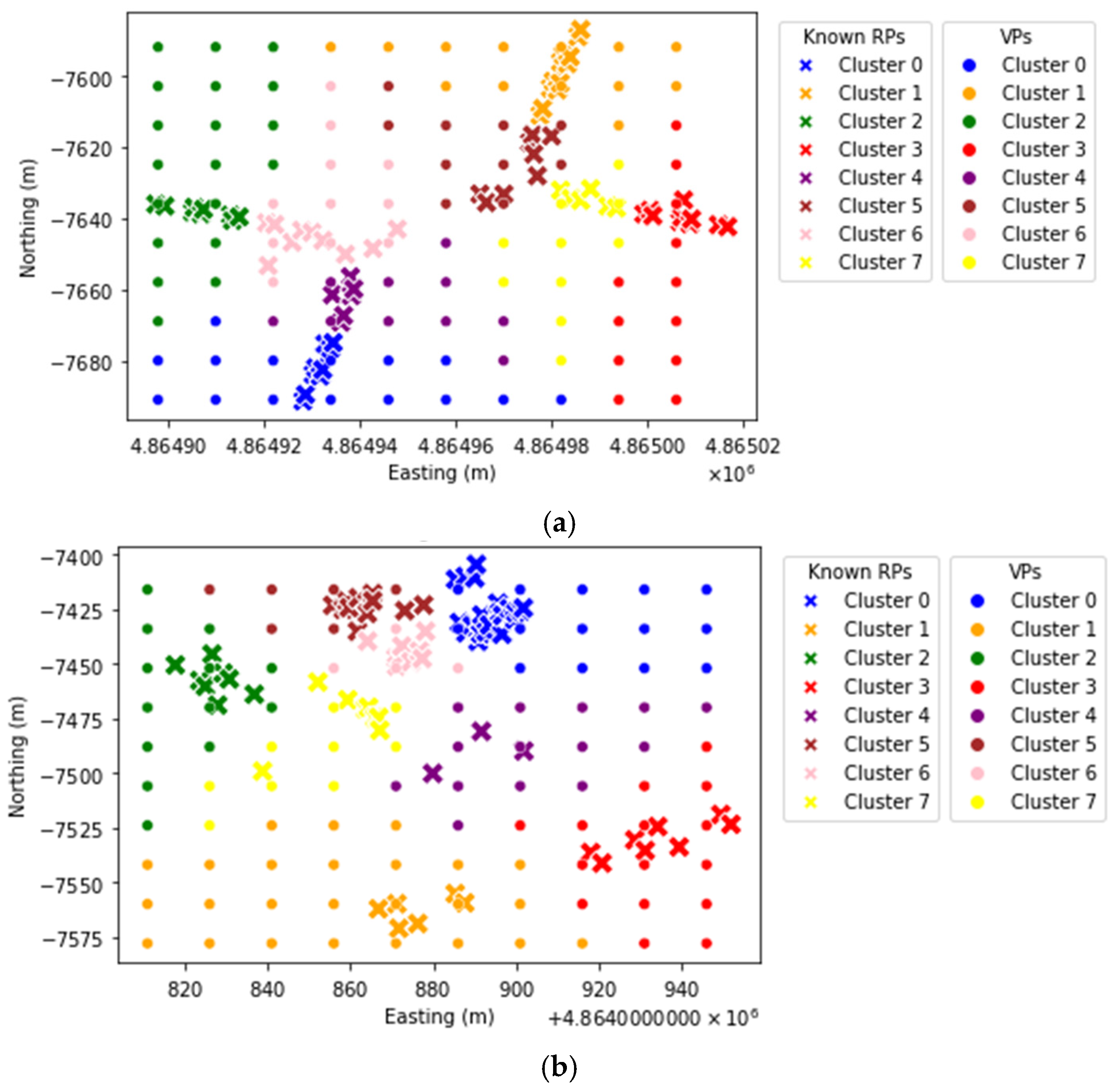
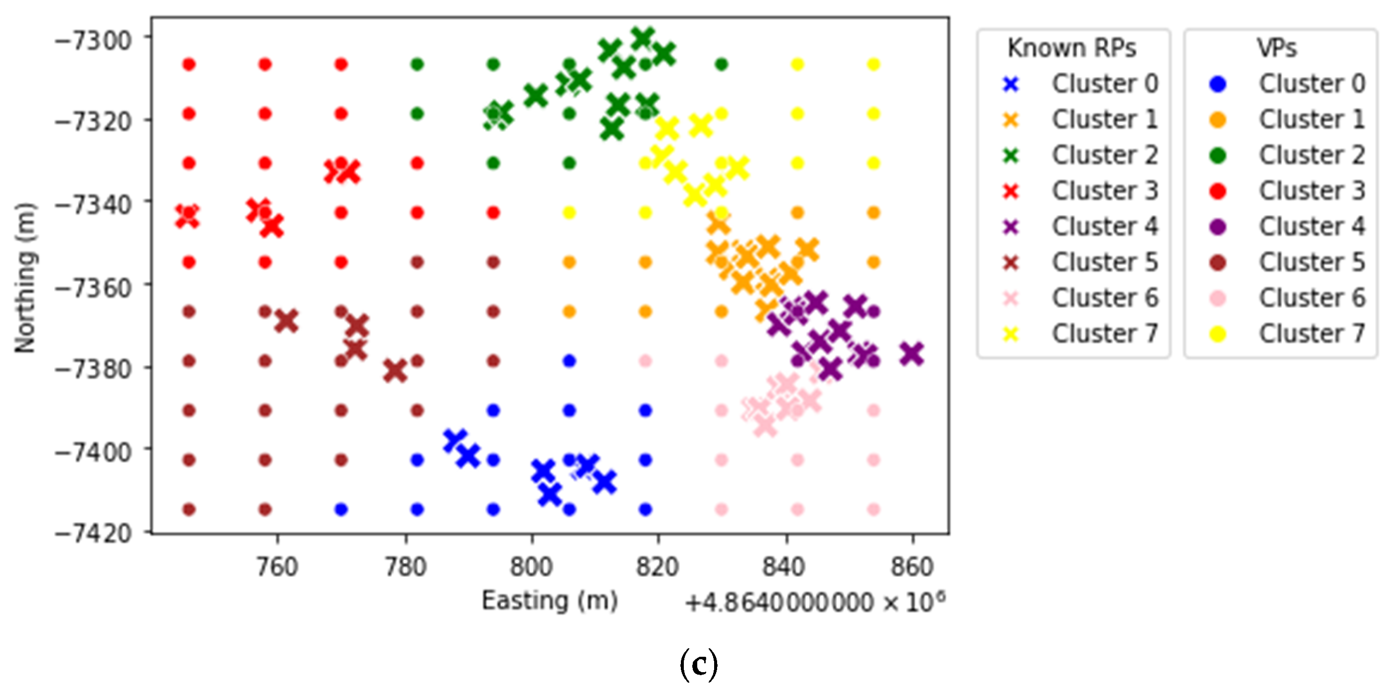
To provide an in-depth analysis, the performance evaluation of the proposed interpolation methods is narrowed down to floor level of each building. Throughout the simulations, the hyperparameters for PCA and TSVD, K-means and IDW are configured as 100 components (p = 100), 8 clusters (c = 8) and 10 nearest neighbors (n = 10), respectively. As mentioned in Section 3, after dimensionality reduction is performed using PCA or TSVD, the proposed DimRedClust invokes K-means clustering to group the known RPs at each floor of each building into several clusters. Afterwards, cluster matching is carried out to select a delegate cluster for each VP with the shortest distance to its cluster centroid. Figure 3 illustrates an example of the clusters of known RPs and VPs for Building 0 Floor 2, Building 1 Floor 0, and Building 2 Floor 0, respectively. The “X” points denote the known RPs while the “.” points indicate the VPs.

After the new radio map is established, it is used to train the KNN localization algorithm with K = 1 while during the online phase, the locations of the 1111 testing samples are being predicted accordingly. In this simulation environment, it could be observed that the test points are surrounded by a high density distribution of reference points in the area for each floor of each building. Thus, K = 1 is adopted in our simulations. Similar performance trend is still observed even if a larger value of K is chosen.

Table 2. RMSE of the easting, northing, and positioning error along with the average positioning error for each floor of each building.

Building	Floor	RMSE	IDW	PCA-IDW	TSVD-IDW	PCA-K-Means-IDW	TSVD-K-Means-IDW
0	0	Easting (m)	9.4416	8.6225	8.9315	8.3859	8.2659
		Northing (m)	14.7595	13.3795	14.1189	12.8554	12.3858
		Positioning Error (m)	17.5210	15.9172	16.7067	15.3488	14.8907
		Average Positioning Error (m)	12.8447	11.3212	11.7703	11.1543	10.7624
	1	Easting (m)	11.7109	9.6786	10.1641	6.9290	6.9693
		Northing (m)	10.5238	9.9266	9.7190	10.7048	10.4493
		Positioning Error (m)	15.7447	13.8641	14.0630	12.7516	12.5602
		Average Positioning Error (m)	10.6407	9.3495	9.5337	8.6490	8.5688
	2	Easting (m)	10.219	9.0521	9.0229	6.5435	6.5338
		Northing (m)	10.0285	9.6556	9.5815	6.607	6.4915
		Positioning Error (m)	14.3178	13.2352	13.1612	9.2989	9.2103
		Average Positioning Error (m)	10.4779	9.3639	9.2744	7.3165	7.2368
	3	Easting (m)	11.0204	8.8976	8.7323	8.0133	7.8294
		Northing (m)	9.2817	7.5031	7.4354	7.6515	7.5851
		Positioning Error (m)	14.4083	11.6389	11.4690	11.0796	10.9011
		Average Positioning Error (m)	10.3945	8.3853	8.1487	7.9698	7.7332
1	0	Easting (m)	19.1633	18.8355	18.8355	16.5722	16.5722
		Northing (m)	20.6161	20.0613	20.0613	23.3360	23.3360
		Positioning Error (m)	28.1470	27.5178	27.5178	28.6218	28.6218
		Average Positioning Error (m)	22.8716	21.3027	21.3027	20.6183	20.6183
	1	Easting (m)	15.756	16.4022	16.5623	14.5905	14.2651
		Northing (m)	18.0366	15.3201	15.1860	14.4555	14.2278
		Positioning Error (m)	23.9493	22.4441	22.4705	20.5388	20.1475
		Average Positioning Error (m)	18.2782	17.6605	17.6604	16.0125	15.6671
	2	Easting (m)	24.5545	24.7884	24.8481	24.4649	24.5011
		Northing (m)	13.0135	14.4692	14.4329	13.8393	13.7363
		Positioning Error (m)	27.7898	28.7023	28.7356	28.1080	28.0890
		Average Positioning Error (m)	19.1628	20.0837	20.2200	19.6864	19.6534
	3	Easting (m)	15.5852	15.7281	15.8921	12.8963	12.8963
		Northing (m)	17.0811	17.4297	17.6340	14.7195	14.7195
		Positioning Error (m)	23.1228	23.4770	23.7385	19.5698	19.5698
		Average Positioning Error (m)	15.8137	16.7522	17.0843	13.5668	13.5668
2	0	Easting (m)	17.9662	16.5076	16.5076	13.3441	13.3441
		Northing (m)	20.2671	19.7827	19.7827	17.4998	17.4998
		Positioning Error (m)	27.0839	25.7654	25.7654	22.0070	22.0070
		Average Positioning Error (m)	17.2819	15.7411	15.7411	12.7154	12.7154
	1	Easting (m)	13.2959	13.1762	12.9223	11.9471	11.9486
		Northing (m)	12.071	11.7508	11.5148	12.9875	13.0040
		Positioning Error (m)	17.9580	17.6548	17.3083	17.6468	17.6599
		Average Positioning Error (m)	14.6222	14.2529	13.7925	13.6007	13.6349
	2	Easting (m)	15.7205	14.0292	13.9836	12.0564	12.1975
		Northing (m)	19.9843	20.3055	19.8579	17.7979	17.6906
		Positioning Error (m)	25.4265	24.6806	24.2874	21.4970	21.4881
		Average Positioning Error (m)	20.6346	19.9707	19.6288	16.7889	16.7773
	3	Easting (m)	10.7117	10.9263	10.9263	10.4662	10.7010
		Northing (m)	13.7748	13.7032	13.7032	11.7456	11.7663
		Positioning Error (m)	17.4495	17.5260	17.5260	15.7321	15.9046
		Average Positioning Error (m)	14.4646	14.7802	14.7802	13.1424	13.2958
	4	Easting (m)	19.4505	18.2221	18.4556	17.2034	17.4443
		Northing (m)	17.6151	19.0586	19.0959	15.7172	16.0164
		Positioning Error (m)	26.2415	26.3681	26.5568	23.3021	23.6818
		Average Positioning Error (m)	22.5599	22.1277	22.5415	19.1979	19.5443
Overall		Easting (m)	13.7705	12.9406	12.9779	11.5283	11.4887
		Northing (m)	12.9225	12.6407	12.6203	11.4905	11.3666
		Positioning Error (m)	18.8843	18.0900	18.1024	16.2768	16.1614
		Average Positioning Error (m)	13.5163	12.7502	12.7502	11.4205	11.3180

shows the RMSE of the easting and northing along with the average positioning error for each floor of each building with different radio map interpolation schemes applied.

From Table 2, it is observed that for most of the scenarios, PCA-IDW and TSVD-IDW under the proposed DimRed interpolation scheme both result in a lower average positioning error than the baseline IDW. Most importantly, for almost all of the scenarios considered, PCA-K-means-IDW and TSVD-K-means-IDW under the proposed DimRedClust interpolation scheme resulted in improved indoor localization performance compared to baseline IDW. Similar improvement trends are also observed for the RMSE of the easting and northing when comparing between the proposed DimRed and DimRedClust interpolation schemes with the baseline IDW. For PCA-K-means-IDW, the improvement in average positioning error ranges approximately from −2.73% to 30.17%, while for TSVD-K-means-IDW, the improvement in average positioning error ranges from approximately −2.56% to 30.93% for the scenarios investigated. This could be considered even more significant than that of PCA-IDW and TSVD-IDW where the performance gain of the average positioning error ranges from −5.93% to 19.33% and −8.03% to 21.61%, respectively. Apart from that, compared to the baseline IDW, the proposed PCA-K-means-IDW, TSVD-K-means-IDW, PCA-IDW, and TSVD-IDW techniques resulted in a performance gain in terms of average positioning error of up to 15.51%, 16.26%, 5.67%, and 5.67%, respectively, as an overall. Thus, this observation implies that clustering could further enhance indoor localization performance.

Upon comparing the PCA and TSVD based dimensionality reduction techniques, it is observed that the performance of both techniques for the scenarios investigated are very similar. More specifically, the TSVD method does not result in a more significant improvement in the indoor localization performance over PCA method since TSVD is originally known to work well when the dataset is sparse. However, in this work, since the missing RSS values in the dataset are all replaced with a RSS value that is slightly lower than the weakest RSS value detected from the APs, the dataset is no longer considered sparse. Hence, TSVD does not exhibit much performance advantage here.

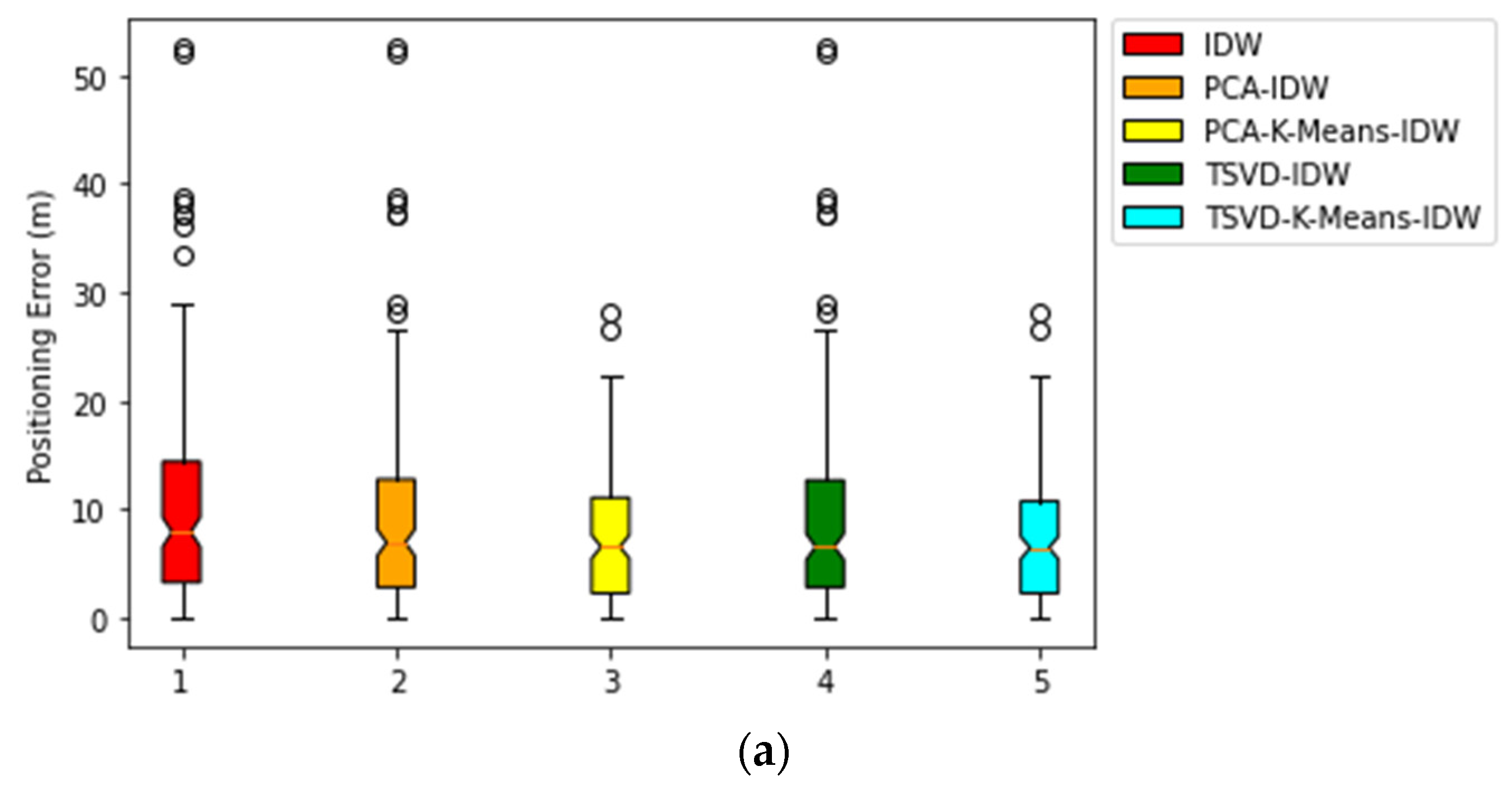
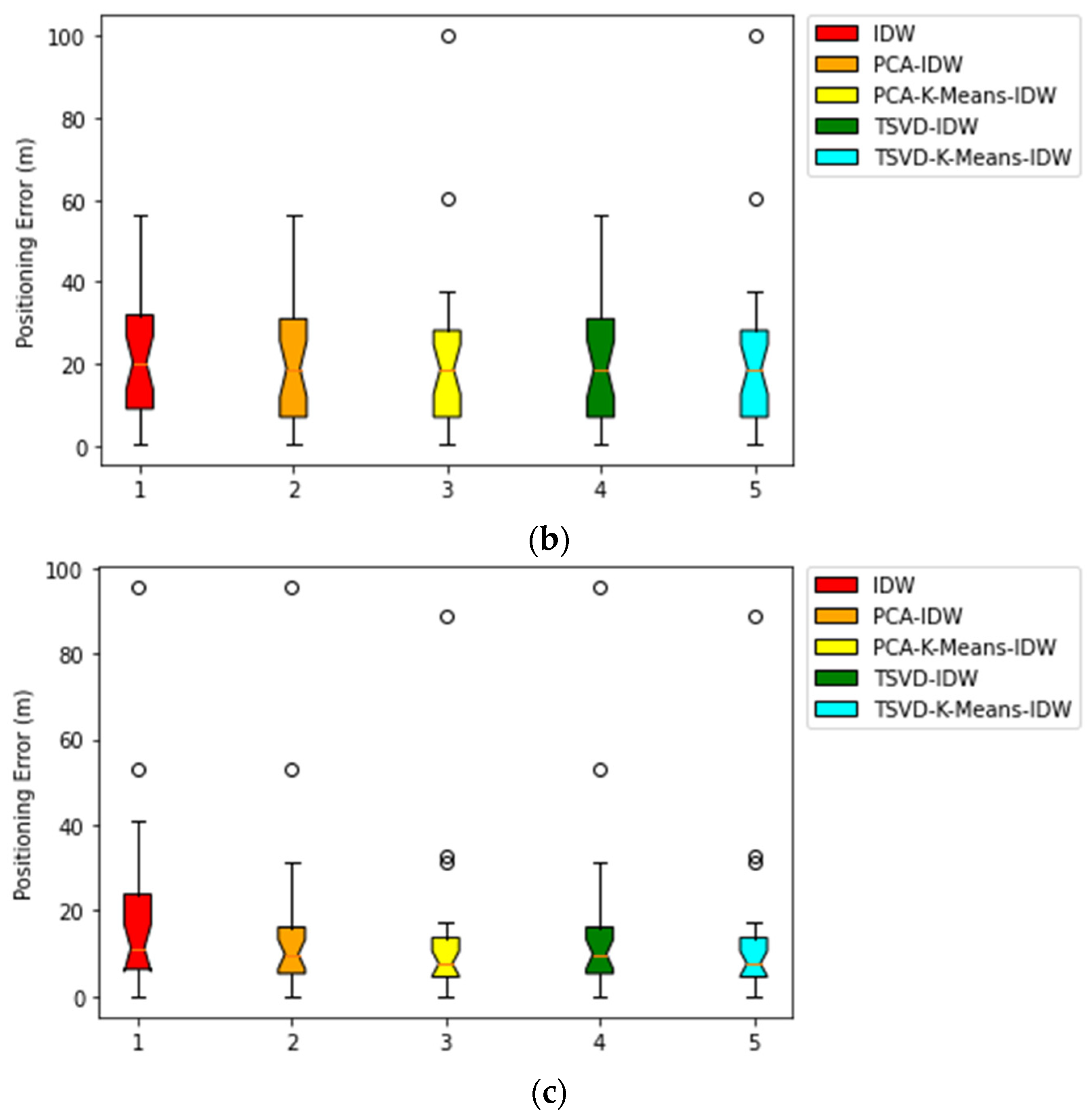
Meanwhile, from the boxplots shown in Figure 4 below, a comparison could be made between the 75th percentiles of the baseline IDW interpolation with those of PCA-IDW and PCA-K-means-IDW for Building 0 Floor 2, Building 1 Floor 0, and Building 2 Floor 0, respectively. Based on the 75th percentiles for the three scenarios presented, it is observed that the PCA-K-means-IDW technique is the best performer among all the other techniques, followed by PCA-IDW and baseline IDW with the worst performance in terms of its highest 75th percentile. For Building 0 Floor 2, the 75th percentile decreases from 14.3882 m for IDW to 12.7461 m for PCA-IDW and 11.0563 m for PCA-K-means-IDW; for Building 1 Floor 0, the 75th percentile decreases from 31.6506 m for IDW to 29.7646 m for PCA-IDW and 27.9245 m for PCA-K-means-IDW, while for Building 2 Floor 0, the 75th percentile decreases from 24.1827 m for IDW to 18.5572 m for PCA-IDW and 13.7196 m for PCA-K-means-IDW, respectively.

The IDW interpolator (initially with a particular number of nearest neighbors fixed) will adjust its number of nearest neighbors according to the number of instances available in each cluster during interpolation. This avoids taking faraway points that belong to another cluster into consideration when interpolating, although that faraway point is also considered as one of the nearest neighbors so as to eliminate its adverse influence in the process of interpolating for a VP. In other words, the selection of known RPs when interpolating for a VP might now be different due to this reason when comparing the interpolation schemes with and without clustering. Thus, this causes the proposed DimRedClust interpolation scheme to outperform both the proposed DimRed interpolation scheme and the baseline IDW interpolation.

In this work, the baseline scheme considered is IDW interpolation and all the proposed techniques (DimRed and DimRedClust) also adopt the same interpolation method as that of the baseline scheme. However, apart from the IDW interpolation, the proposed DimRed technique also performs dimensionality reduction prior to the interpolation while the proposed DimRedClust employs both the dimensionality reduction and clustering before interpolating the radio map. By extracting the essential features from the RSS data via dimensionality reduction, both the proposed DimRed and DimRedClust could effectively minimize the influence of noise and outliers that initially present in the high-dimensional fingerprint matrix while reducing the computational cost. On the other hand, clustering could further improve the performance of DimRedClust by confining the selection of nearest neighbors to only the known RPs located in the same cluster. For these reasons, regardless of the number of nearest neighbors used for KNN localization, distribution of RSS in space, or known reference points, the proposed techniques could still outperform the baseline counterpart due to the performance advantages resulting from dimensionality reduction and clustering.

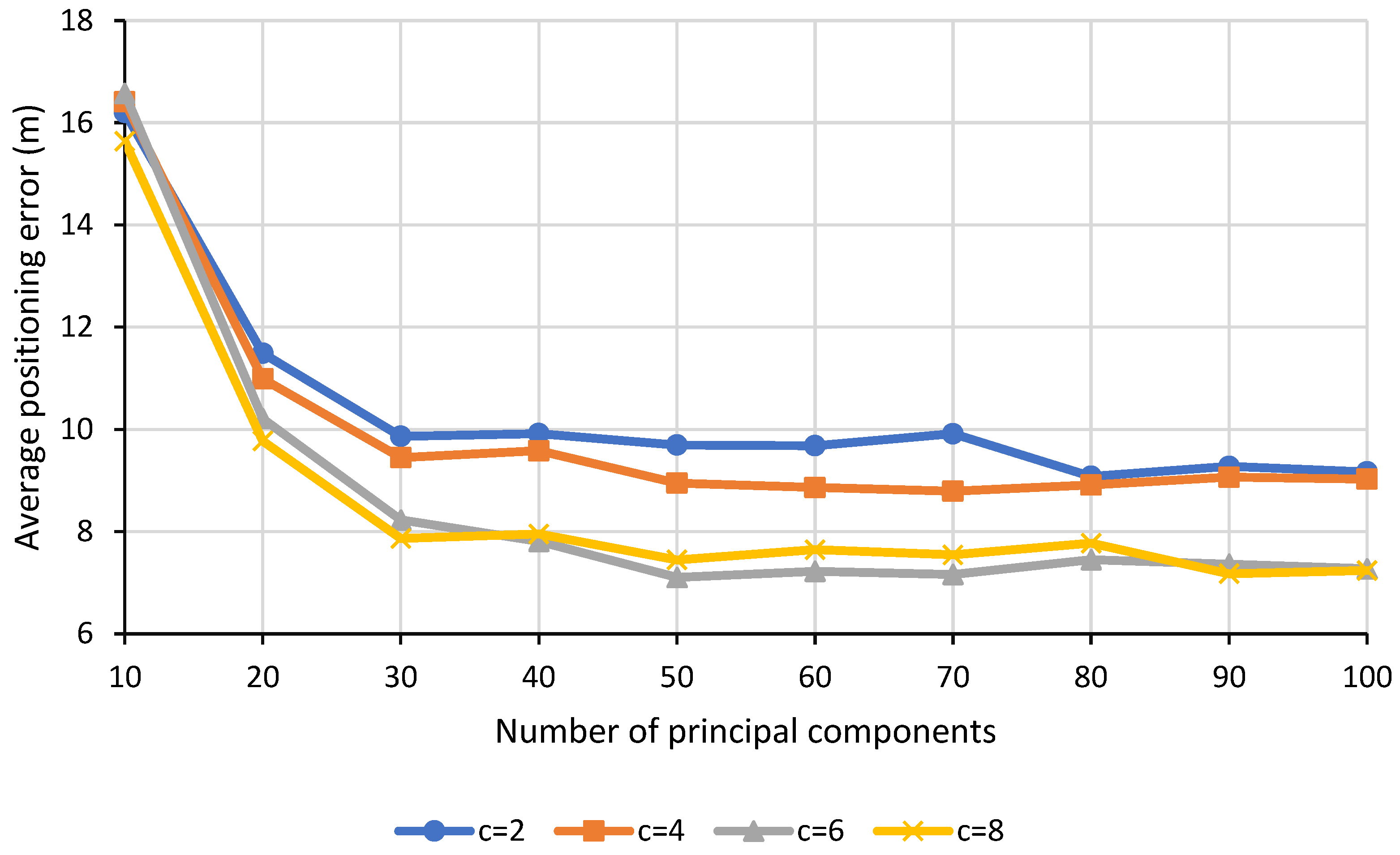
5.3. Effects of Hyperparameters

This subsection investigates the effects of the 3 hyperparameters, namely the number of components p, number of clusters c and number of nearest neighbors n of IDW on the performance of the indoor localization in terms of the average positioning error for B0F2 scenario. The line plots for PCA-K-means-IDW technique are as shown in Figure 5, Figure 6 and Figure 7 while the line plots for TSVD-K-means-IDW technique are as illustrated in Figure 8, Figure 9 and Figure 10 below.

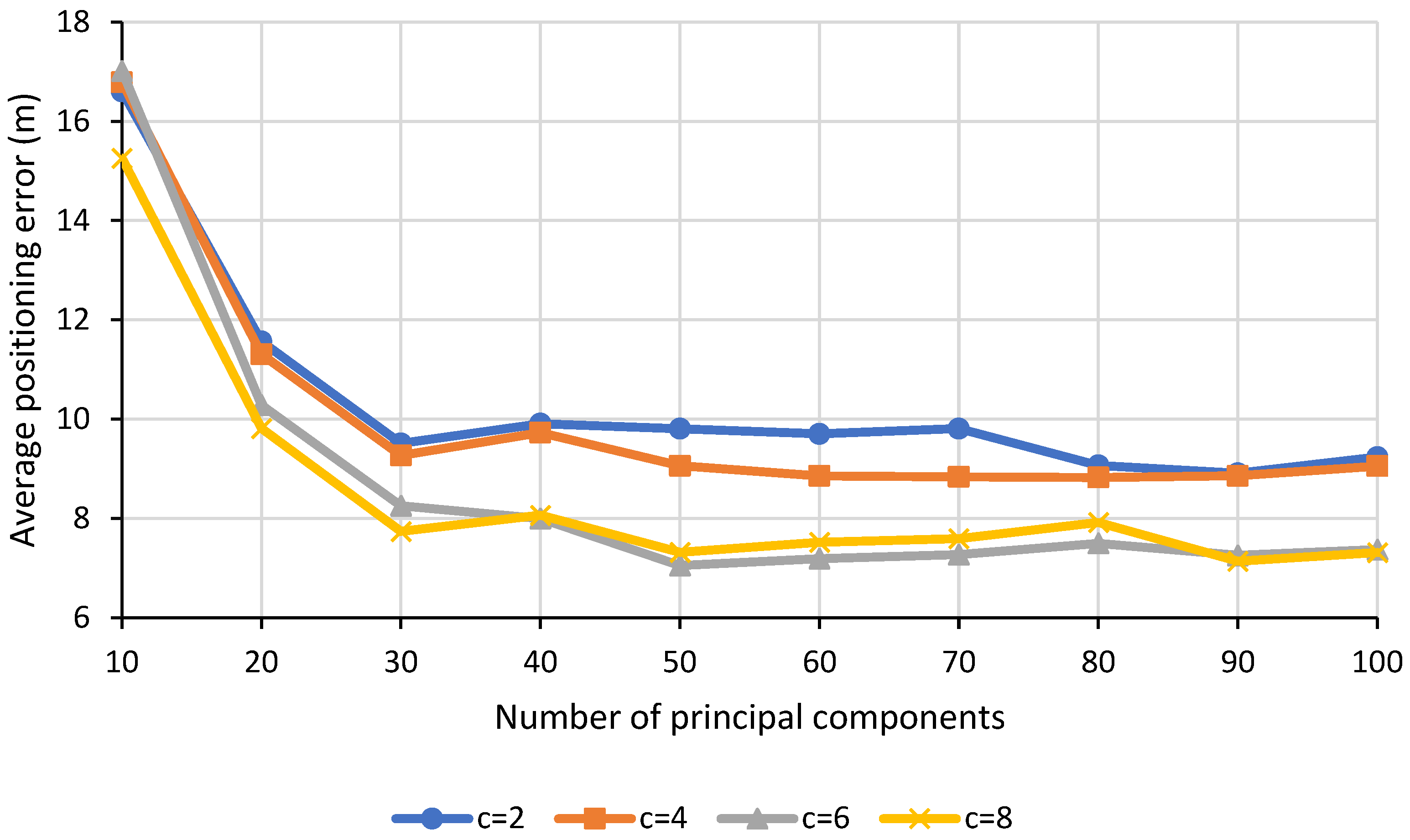
From the line plot shown in Figure 5, it is observed that as the number of principal components increases, the average positioning error decreases and eventually converges as the number of the principal components continues to increase beyond 50. In the real-world scenario which involves a large indoor environment, a large number of APs would generally be deployed to provide ubiquitous coverage. However, most of the time, not all APs are useful and such redundancy of APs might result in biased estimation during the RSS interpolation. This in turn degrades the quality of the interpolated radio map and hence, the accuracy of indoor localization. In view of that, by extracting only the informative features via dimensionality reduction prior to interpolation, the number of detected APs could be reduced by multiple folds. Ultimately, the quality of the interpolated radio map would be enhanced, and the average positioning error would also improve.

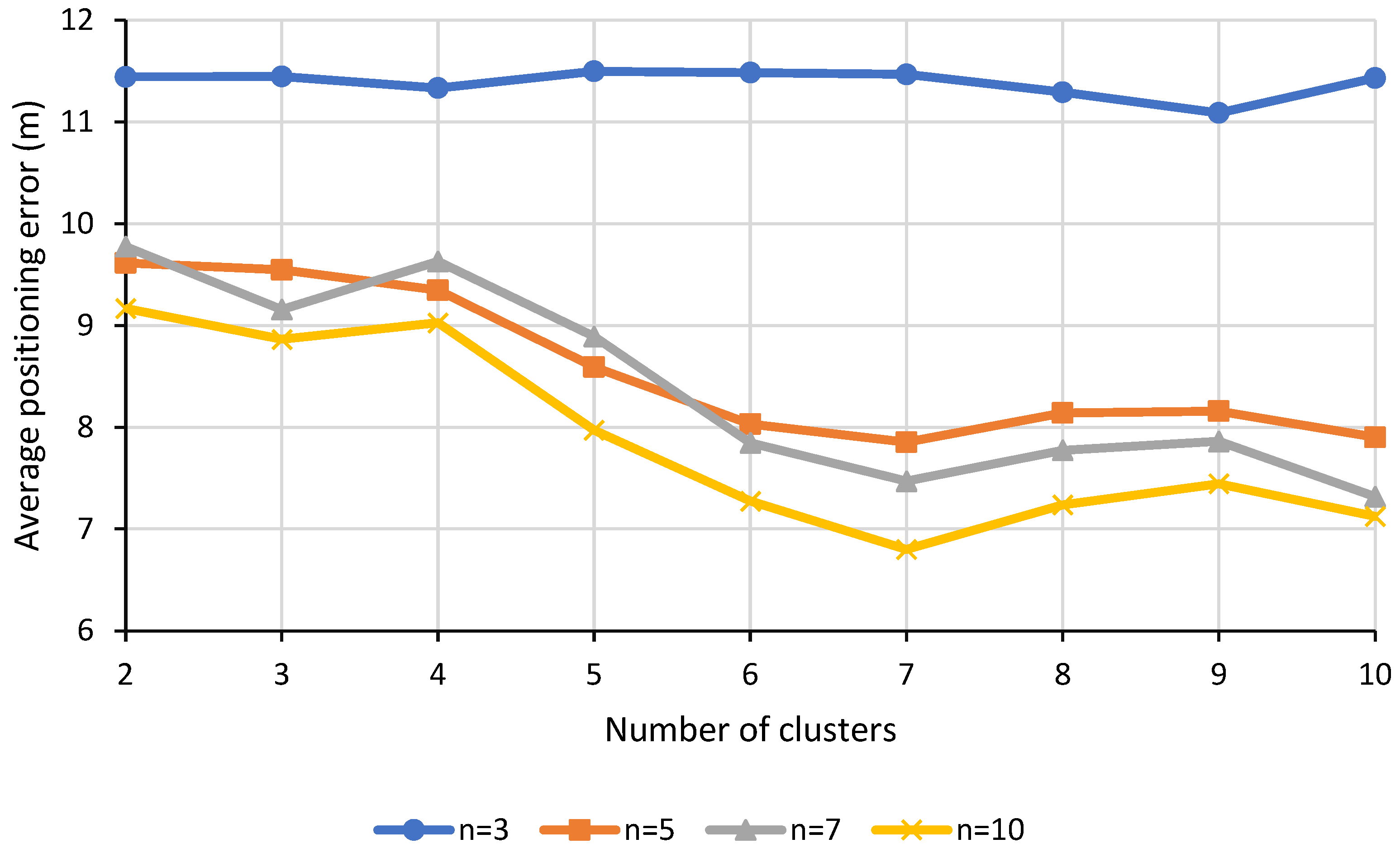
Meanwhile, from Figure 6, as the number of clusters increases, the average positioning error decreases until it reaches an optimum value before saturating. This implies that a slightly higher number of clusters helps to improve the indoor localization performance. Without clustering, inappropriate known RPs that are located far from the VP might be selected as the nearest neighbors and also contribute to the RSS interpolation. As a result, RSS fluctuation due to the inclusion of those inappropriate nearest neighbors might adversely affect the RSS interpolation of the VPs. Hence, clustering is essential to confine the selection of nearest neighbors to only the known RPs located in the same cluster. Note that when the number of nearest neighbors is small, i.e., n = 3, the average positioning error exhibits a different trend as compared to those with a higher number of nearest neighbors. This is because clustering does not exhibit much advantage in this case since the probability for faraway known RPs located in different cluster to be selected as one of the nearest neighbors for the RSS interpolation is extremely low with a smaller number of nearest neighbors being selected. Thus, regardless of the number of clusters, the average positioning error remains almost constant throughout.

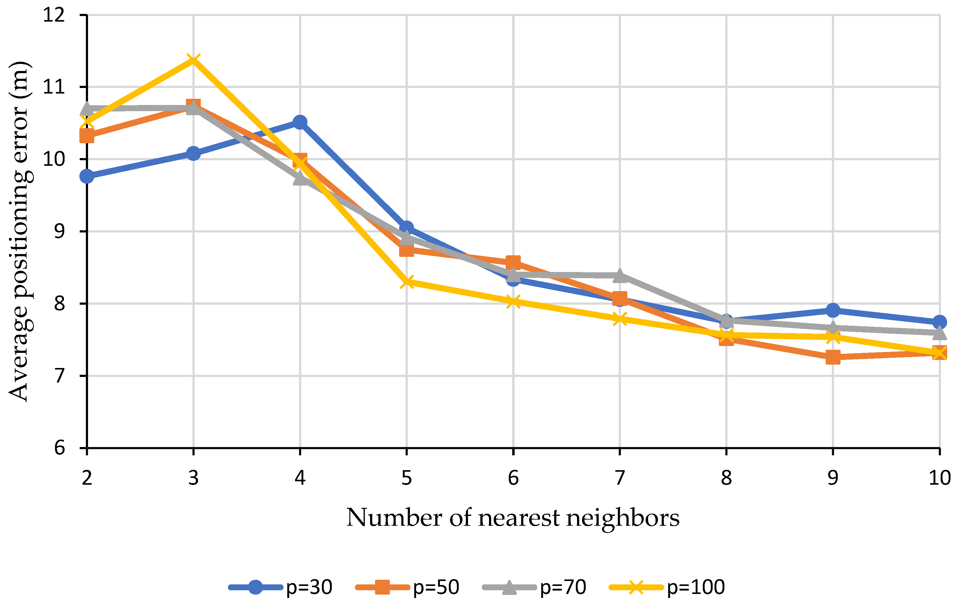
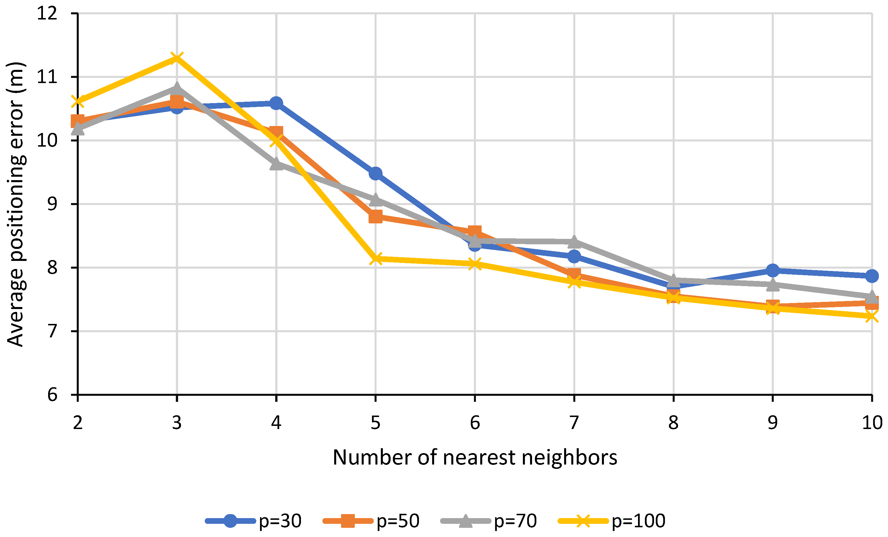
From Figure 7, it can be observed that the average positioning error initially fluctuates when the number of nearest neighbors is low but possesses a decreasing trend afterwards as the number of nearest neighbors continues to increase. This suggests that a higher number of nearest neighbors could be used for this scenario. With a moderately higher number of nearest neighbors contributing to the RSS interpolation, the effect of outliers on the RSS interpolation could be suppressed and this will thus result in a less biased RSS estimation. With the enhancement in the quality of the interpolated radio map, the performance of the indoor localization in terms of its average positioning error will also improve.

Comparing Figure 5, Figure 6 and Figure 7 with Figure 8, Figure 9 and Figure 10 respectively, it is noticed that the line plots produced by the TSVD-K-means-IDW technique possess similar trend to that of the PCA-K-means-IDW technique since both techniques resulted in similar indoor localization performance in terms of their average positioning error.

6. Conclusions

In this paper, two interpolation methods, namely DimRed and DimRedClust, are proposed for the construction of an enhanced radio map that is robust against environmental noise and RSS fluctuations. In a large indoor environment where not all of the detected APs are useful for indoor localization, dimensionality reduction is employed in both proposed interpolation schemes to extract key features with maximal information for better feature representation besides suppressing the impact of outliers and noise. Apart from that, the proposed DimRed and DimRedClust interpolation schemes are also beneficial in large indoor environment since dimensionality reduction helps to save storage in resource constrained mobile devices used for indoor positioning.

Additionally, in the proposed DimRedClust interpolation scheme, the known RPs are further grouped into several clusters such that the RPs closer to each other will possess similar RSS characteristics. The RSS for the VPs in each cluster are then interpolated based on the nearest known RPs located in the same cluster to prevent the inclusion of nearest known RPs located faraway which might introduce RSS fluctuations into the RSS interpolation of the VPs. Based on the new radio map generated, indoor localization is performed via the KNN localization algorithm.

An extensive and in-depth analysis is carried out using a real-world multi-building and multi-floor dataset. Our results demonstrate that the proposed DimRedClust interpolation scheme outperforms the other proposed DimRed interpolation scheme, while both proposed schemes outperform the baseline IDW interpolation by up to 30.17% for PCA-K-means-IDW, 30.93% for TSVD-K-means-IDW, 19.33% for PCA-IDW and 21.61% for TSVD-IDW, respectively. Meanwhile, from the investigation of the effects of the hyperparameters, it is confirmed that a moderately higher number of principal components, clusters, and nearest neighbors of IDW could help to improve the indoor localization performance in terms of average positioning error. With numerous merits shown, it could be concluded that the proposed DimRed and DimRedClust interpolation schemes are indeed practical and promising for deployment in real-world scenarios to cover large scale indoor positioning.