Method for Direct Localization of Multiple Impulse Acoustic Sources in Outdoor Environment

Abstract

A method for the direct outdoor localization of multiple impulse acoustic sources by a distributed microphone array is proposed. This localization problem is of great interest for gunshot, firecracker and explosion detection localization in a civil environment, as well as for gun, mortar, small arms, artillery, sniper detection localization in military battlefield monitoring systems. Such a kind of localization is a complicated technical problem in many aspects. In such a scenario, the permutation of impulse arrivals on distributed microphones occurs, so the application of classical two-step localization methods, such as time-of-arrival (TOA), time-difference-of-arrival (TDOA), angle-of-arrival (AOA), fingerprint methods, etc., is faced with the so-called association problem, which is difficult to solve. The association problem does not exist in the proposed method for direct (one-step) localization, so the proposed method is more suitable for localization in a given acoustic scenario than the mentioned two-step localization methods. Furthermore, in the proposed method, direct localization is performed impulse by impulse. The observation interval used for the localization could not be arbitrarily chosen; it is limited by the duration of impulses. In the mathematical model formulated in the paper, atmospheric factors in acoustic signal propagation (temperature, pressure, etc.) are included. The results of simulations show that by using the proposed method, centimeter localization accuracy can be achieved.

1. Introduction

Localization of multiple impulse acoustic sources is of great interest for gunshot, mortar, artillery, sniper, firecracker and explosion detection localization in civil environments as well as in military battlefield monitoring systems [1,2,3,4,5,6,7,8,9,10,11,12,13].

That is a very challenging and complicated technical problem in many aspects:

• In such a multiple impulse scenario, the permutation of impulse arrivals on distributed microphones occurs, so the application of classical two-step localization methods, such as time-of-arrival (TOA), time-difference-of-arrival (TDOA), angle-of-arrival (AOA), fingerprint methods, etc., is faced with the so-called association problem [14].
• In such a multi-source signal scenario, direct localization is performed, impulse by impulse, so the observation interval used for the localization cannot be arbitrarily chosen. It is limited by the duration of impulses.
• Factors in acoustic signal propagation (temperature, pressure, etc.) affect the impulse shape, duration, and amplitude at the receiver side. This effect is not the same for all the array’s microphones because of the different propagation delays from the source to different microphones. It complicates the estimation of the localization parameters and it should be included in the system and signal model.

Thanks to the analogy of mathematical models of signal superposition at the antenna and microphone arrays, the methods for the localization of radio transmitters are applicable for the localization of acoustic sources and vice versa. It should be noted that the acoustic signal at the microphone array is always modeled as a broadband signal in the space–time domain.

Several localization methods have been developed and all can be generally divided into two main groups: two-step (i.e., indirect localization) and one-step (direct localization) methods [15].

In the two-step methods, localization parameters, such as angle of arrival, time of arrival, time difference of arrival or received signal strength, are estimated for each distributed sensor. In the second step, the estimated localization parameters are collected in the fusion center, where localization process is performed. An inherent problem of two-step localization methods is the so-called association problem, which is very difficult to solve.

Theoretically, the performance of two-step localization methods is well studied in the literature [16,17,18,19,20,21,22,23]. This is limited by the signal-to-noise ratio, number of sensors, signal bandwidth, observation interval, etc. The performance of two-step localization methods is significantly degraded in multipath as well as non-line-of-sight (NLOS) environments.

In order to improve the performance of two-step methods, hybrid measurements that combine measurements of different signal parameters were performed in the first step [16]. Suitable combinations of measuring different parameters for different environments and conditions in which the localization takes place are as follows:

• For indoor environment and the non-line-of-sight (NLOS) condition, it is convenient to combine TOA/RSS and TDOA/RSS measurements. The advantage of this hybrid method is that it requires relatively simple hardware.
• If the source is in the proximity of a sensor and it is necessary to perform localization with one sensor in an indoor environment and NLOS conditions, it is convenient to combine TOA/AOA and TDOA/AOA.
• If the source is moving, it is convenient to use TDOA/frequency-difference-of-arrival (FDOA). It is complementary to TDOA for location and velocity assessment.
• For NLOS conditions, when it is necessary to perform data fusion, it is convenient to use TOA/TDOA.

Direct localization methods are of the new date [24,25,26]. In [24], Weiss proposed a novel approach for the localization of narrowband radio transmitters, named as direct position determination (DPD). In the paper, he claimed that DPD has slightly better performance than the performance of two-step localization methods at lower signal-to-noise ratios. The key advantage of the proposed DPD method is that the problem of association in DPD approach does not exist.

The localization of multiple impulse acoustic sources is analogous to the localization in multiuser impulse Ultra WideBand (UWB) systems [27].

The main advantage of the proposed one-step method is that the problem of the association of impulses from different acoustic sources at the microphone array is completely eliminated. The sources of all impulses that are successfully detected on the microphone array can be localized directly based on the raw signal samples (in a single step), unlike in two-step methods, which rely on some intermediate parameter estimates (obtained in a previous step). The impulse detection in a multi-source environment is often difficult because the impulses of different sound sources can overlap in individual channels of a microphone array. The method allows the successful localization of all sources, regardless of whether the impulses on individual microphones overlap or not. These two characteristics of the proposed method enable successful work in a multi-source environment.

In outdoor localization, the phenomena that occur during the propagation of sound have a great influence on the results of localization [28,29]. The influence of the propagation phenomena is noticeable in all types of microphone arrays [30]. To know the phenomena of sound outdoor propagation means to know the influence of the atmosphere, soil and obstacles on the sound wave. Various phenomena, such as soil attenuation and meteorological factors that affect atmospheric attenuation in the propagation of sound outdoors, are theoretically known and standardized [31,32,33,34,35]. The proposed method takes into account the atmospheric attenuation, i.e., all meteorological parameters that affect it.

Most papers from the literature focus on single-source localization in the isotropic environment. The method proposed in the paper is applied to multiple-source localization in a small area, where an isotropic environment is assumed. In the proposed algorithm, propagation effects are modeled from each hypothetical source location to each microphone, separately. So, the algorithm can be applied for localization in an anisotropic environment. This is one of the novelties of the paper.

The proposed method is more computationally complex then the existing two-step methods, if we do not count the numerical complexity of the association problem that the two-step methods suffer from. Thus, a more powerful computer platform is required, while the other elements, such as synchronization and A/D conversion, do not differ from the localization system based on the TOA/TDOA principle, and they do not represent a technological barrier for the implementation of the proposed localization method. The key difference is that the estimation of localization parameters in the TDOA system is performed on distributed sensors, while in the direct localization system, the acquired signal samples from all stations are delivered to the fusion center where the localization is performed.

The paper is organized in the following way. Section 2 discusses the mathematical model of the signal and describes its acquisition on a microphone array. The process of impulse sound sources localization as a one-step method, taking into account the phenomena of sound absorption in the atmosphere during propagation, is given in Section 3. Section 4 presents the obtained results and demonstrates performance of the proposed method in the process of impulse sound sources localization. The results point out the algorithm’s ability to operate in an environment with multiple impulse sound sources, as well as the quantitative and qualitative performance of the method. Section 5 concludes the paper.

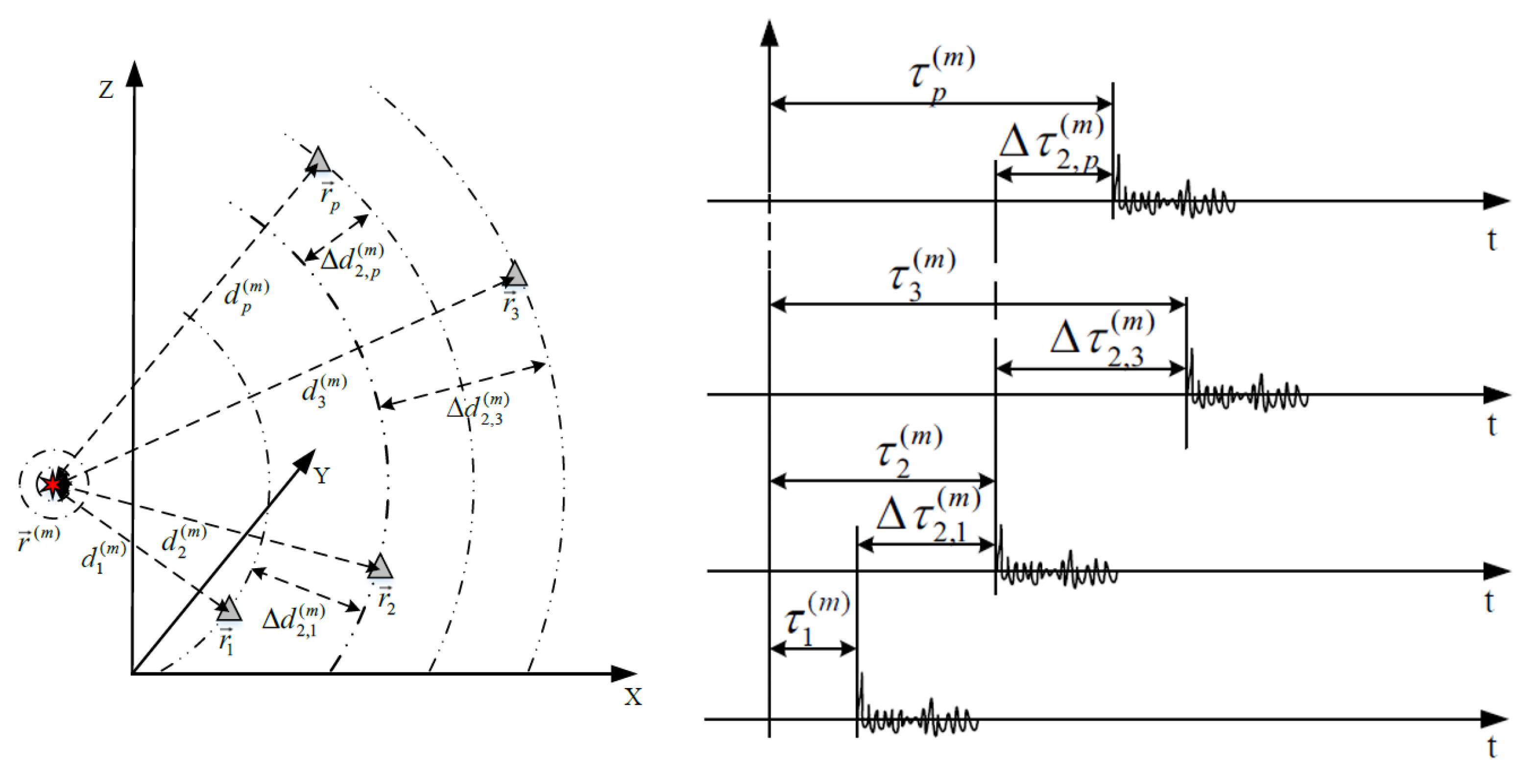
2. Signal Model

Assume a scenario in the region of interest as in Figure 1. A spatially distributed microphone array consists of P microphones arranged in locations described by vectors ${\overrightarrow{r}}_p=\left(x_p,y_p,z_p\right)$, where $p\in \left\{1,2,\dots ,P\right\}$. The number of acoustic signals superimposed on the microphone array is M. The actual source locations of the acquired signal are described by vectors ${\overrightarrow{r}}^{\left(m\right)}=\left(x^{\left(m\right)},y^{\left(m\right)},z^{\left(m\right)}\right)$, where $m\in \left\{1,2,\dots ,M\right\}$.

The continuous signal model in the time domain (in physical units: s and Hz) on the p-th microphone can be expressed as follows:

$${\tilde{s}}_p\left(\tilde{t}\right)=\sum _{m=1}^M{\gamma }_p^{\left(m\right)}{\tilde{h}}_p^{\left(m\right)}\left(\tilde{t}\right)⊛{\tilde{s}}_0^{\left(m\right)}\left(\tilde{t}-{\tilde{\tau }}_p^{\left(m\right)}\right){\tilde{w}}_p\left(\tilde{t}\right),$$

(1)

where $\tilde{t}$ is a time in seconds, ${\gamma }_p^{\left(m\right)}$ is the attenuation due to the propagation of the wavefront from the m-th source to the p-th microphone, ${\tilde{h}}_p^{\left(m\right)}\left(\tilde{t}\right)={\mathrm{F}}^{-1}\left\{{\tilde{\beta }}_p^{\left(m\right)}\left(\tilde{f}\right)\right\}$ is the impulse response corresponding to the transfer function ${\tilde{\beta }}_p^{\left(m\right)}\left(\tilde{f}\right)={10}^{{\tilde{b}}_p^{\left(m\right)}\left(\tilde{f}\right)/20}$, where ${\tilde{b}}_p^{\left(m\right)}\left(\tilde{f}\right)$ is the attenuation of the signal from the location of the m-th source to the p-th microphone due to the propagation in the atmosphere, ${\tilde{s}}_0^{\left(m\right)}$ is the signal from the m-th source at the location of the source, ${\tilde{\tau }}_p^{\left(m\right)}$ is the propagation delay of the signal from m-th source to the p-th microphone, and ${\tilde{w}}_p\left(\tilde{t}\right)$ is the noise on the p-th receiving channel. The label ⊛ indicates a convolution.

For easier conversion between the continuous- and discrete-time (digital) mathematical model, the frequency axis will be normalized with the sampling frequency ${\tilde{f}}_{\mathrm{s}}$ and the time axis with the sampling period $1/{\tilde{f}}_{\mathrm{s}}$. So, the normalized sampling frequency is $f_{\mathrm{s}}$. The symbol ∼ (tilde) means that the units in (1) are physical units. The normalized continuous-time signal model $s_p\left(t\right)$ on the p-th microphone is given by the following equation:

$$s_p\left(t\right)=\sum _{m=1}^M{\gamma }_p^{\left(m\right)}{h}_p^{\left(m\right)}\left(t\right)⊛s_0^{\left(m\right)}\left(t-{\tau }_p^{\left(m\right)}\right)w_p\left(t\right),$$

(2)

where the units without a tilde have the same meaning as the corresponding units from (1), except that they are normalized in the manner described above. In the remaining text, the normalized model is used (i.e., symbols without tilde).

We do not consider the localization and tracking of moving targets. Additionally, microphones are stationary and the proposed method based on the scalar product is robust to small Doppler shifts. Therefore, the model does not include the Doppler effect.

The signal model uses the time delay between the source and the microphone when the ${\tau }_p^{\left(m\right)}$ is defined as

$${\tau }_p^{\left(m\right)}=d_p^{\left(m\right)}{\tilde{f}}_{\mathrm{s}}/v=∥{\overrightarrow{r}}^{\left(m\right)}-{\overrightarrow{r}}_p∥{\tilde{f}}_{\mathrm{s}}/v.$$

(3)

When $\Delta {\tau }_{p,q}^{\left(m\right)}$ is

$$\Delta {\tau }_{p,q}^{\left(m\right)}={\tau }_p^{\left(m\right)}-{\tau }_q^{\left(m\right)}=\left(∥{\overrightarrow{r}}^{\left(m\right)}-{\overrightarrow{r}}_p∥-∥{\overrightarrow{r}}^{\left(m\right)}-{\overrightarrow{r}}_q∥\right){\tilde{f}}_{\mathrm{s}}/v,$$

(4)

the model employs the relative time delays between two microphones, p and q.

The speed of sound propagation $v[\mathrm{m}/\mathrm{s}]$ is defined as

$$v=343.2(1+1.0016h)\sqrt{(273.15+T)/T_r},$$

(5)

where $T{[}^{\circ }\mathrm{C}]$ is the air temperature, $h[\%]$ is the molar concentration of water vapor, and $T_r=293.15\mathrm{K}$ is the reference air temperature [31].

The attenuation of the acoustic signal in the atmosphere is represented by the expression $b_p^{\left(m\right)}=\alpha d_p^{\left(m\right)}$ [31]. The attenuation coefficient in the atmosphere $\alpha \left[\mathrm{dB}/\mathrm{m}\right]$ can be defined by the following expressions:

$$\begin{array}{c}\alpha =8.86{\tilde{f}}^2\left(\left[1.84\times {10}^{-11}{(p_a/p_r)}^{-1}{((273.15+T)/T_r)}^{1/2}\right]+{\alpha }_1\right),\\ {\alpha }_1={((273.15+T)/T_r)}^{-5/2}\times ({\alpha }_2+{\alpha }_3),\\ {\alpha }_2=0.01275\left[\exp (-2239.1/(273.15+T\left)\right)\right]\left[{\tilde{f}}_{\mathrm{ro}}/\left({\tilde{f}}_{\mathrm{ro}}^2+{\tilde{f}}^2\right)\right],\\ {\alpha }_3=0.01068\left[\exp (-3352/(273.15+T\left)\right)\right]\left[{\tilde{f}}_{\mathrm{rN}}/\left({\tilde{f}}_{\mathrm{rN}}^2+{\tilde{f}}^2\right)\right].\end{array}$$

(6)

In (6), $\tilde{f}\left[\mathrm{Hz}\right]$ is the frequency of sound, $p_a\left[\mathrm{kPa}\right]$ is the ambient atmospheric pressure, $p_r=101.325\mathrm{kPa}$ is the reference value of ambient pressure, ${\tilde{f}}_{\mathrm{ro}}\left[\mathrm{Hz}\right]$ is the frequency of oxygen relaxation, and ${\tilde{f}}_{\mathrm{rN}}\left[\mathrm{Hz}\right]$ is the frequency of nitrogen relaxation. These frequencies can be described by the following equations:

$${\tilde{f}}_{\mathrm{ro}}=(p_a/p_r)\left\{24+\left[\left(4.04\times {10}^4\times h\right)(0.02+h)/(0.391+h)\right]\right\},$$

(7)

$${\tilde{f}}_{\mathrm{rN}}=(p_a/p_r){(T_a/T_r)}^{-\frac{1}{2}}\left(9+280\times h\times \exp \left\{-4.17\times \left[{(T/T_r)}^{-\frac{1}{3}}-1\right]\right\}\right).$$

(8)

In (7) and (8) the molar concentration of the water vapor $h[\%]$ is given by expressions (9):

$$\begin{array}{c}h=h_r(p_{\mathrm{sat}}/p_a),\\ p_{\mathrm{sat}}=p_r{10}^C,\\ C=-6.8346{(T_{01}/T)}^{1.261}+4.6151,\end{array}$$

(9)

where $h_r[\%]$ is relative humidity, $p_{\mathrm{sat}}$ is saturated water vapor pressure, and $T_{01}=273.16\mathrm{K}$ is triple point isotherm temperature.

In the spectral domain, the acquired signal on the microphone array can be written as

$$\mathbf{S}\left(k\right)=\mathbf{A}\left(k\right){\mathbf{S}}_0\left(k\right)+\mathbf{W}\left(k\right),$$

(10)

where $k\in \left\{1-K/2,\dots ,K/2-1\right\}$, where K is the number of spectral components, i.e., $\mathbf{S}\left(k\right)\in {\mathbb{C}}^{P\times 1}$ is the vector of the k-th spectral component of the acoustic signal on the microphone array, $\mathbf{A}\left(k\right)\in {\mathbb{C}}^{P\times M}$ models attenuation and delay of acoustic signals from the locations of sources to all microphones on the k-th spectral component, ${\mathbf{S}}_0\left(k\right)\in {\mathbb{C}}^{M\times 1}$ represents a vector with the k-th spectral component of all acoustic signals at the location of the sources, and $\mathbf{W}\left(k\right)\in {\mathbb{C}}^{P\times 1}$ represents the noise on the k-th spectral component in the receiving channels of the microphone array.

The matrix $\mathbf{A}\left(k\right)$, whose columns are steering vectors that map signals from the source to the microphone array, is denoted as

$$A=\left[\begin{array}{cccc}{a}_1^{\left(1\right)}& a_1^{\left(2\right)}& \cdots & a_1^{\left(M\right)}\\ a_2^{\left(1\right)}& a_2^{\left(2\right)}& \cdots & a_2^{\left(M\right)}\\ ⋮& ⋮& \ddots & ⋮\\ a_P^{\left(1\right)}& a_P^{\left(2\right)}& \cdots & a_P^{\left(M\right)},\end{array}\right]$$

(11)

where $a_p^{\left(M\right)}$ is

$$a_p^{\left(m\right)}={\gamma }_p^{\left(m\right)}{\beta }_p^{\left(m\right)}(k/K)\exp \left(-\mathrm{j}2\pi k{\tau }_p^{\left(m\right)}/K\right).$$

(12)

Vector ${\mathbf{S}}_0\left(k\right)$ is defined as

$${\mathbf{S}}_0\left(k\right)=\left[S_0^{\left(1\right)}\left(k\right),S_0^{\left(2\right)}\left(k\right),\dots ,S_0^{\left(m\right)}\left(k\right),\dots ,S_0^{\left(M\right)}\left(k\right)\right]$$

(13)

where $S_0^{\left(m\right)}\left(k\right)$, $m\in \left\{1,\dots ,M\right\}$, $k\in \left\{1-K/2,\dots ,K/2-1\right\}$ denotes the k-th spectral component of the m-th signal at the location of the source.

3. Direct Localization Algorithm

The proposed localization algorithm is of the search type, which means that a criterion function is calculated over a set of hypothetical locations. The arguments of the function’s maxima are estimated locations of the sources. For an arbitrary hypothetical location, it is defined as ${\overrightarrow{r}}_{\mathrm{H}}=\left(x,y,z\right)\in \mathrm{H}$, where H is the set of all hypothetical locations in which the criterion function is calculated by the localization algorithms. $\left|\mathrm{H}\right|={\mathrm{H}}^{\mathrm{loc}}$, where the symbol $|·|$ denotes the number of the set elements, and ${\mathrm{H}}^{\mathrm{loc}}$ denotes the total number of hypothetical locations, which the localization algorithm searches for. ${\mathrm{H}}^{\mathrm{loc}}$ can be represented as

$${\mathrm{H}}^{\mathrm{loc}}={\mathrm{H}}_x^{\mathrm{loc}}{\mathrm{H}}_y^{\mathrm{loc}},$$

(14)

where ${\mathrm{H}}_x^{\mathrm{loc}}$ and ${\mathrm{H}}_y^{\mathrm{loc}}$ denote the number of hypothetical locations along the x- and y axes, respectively. A search of the region of interest is performed on each hypothetical location for all detected impulses.

The impulse detection for a given threshold value is performed on a given reference channel, $p_{\mathrm{ref}}$, of the acquired signals on the microphone array. For all detected impulses, signal windowing is performed according to the following equation:

$$s_{0\mathrm{SIM}}\left(t\right)=\Pi \left(t\right)s_{p_{ref}}\left(t\right),$$

(15)

where the window function $\Pi \left(t\right)$ is defined as

$$\Pi \left(t\right)=\left\{\begin{array}{cc}1,\hfill & {\mathrm{I}}_{\mathrm{start}}\le t\le {\mathrm{I}}_{\mathrm{stop}}\hfill \\ 0,\hfill & \mathrm{otherwise}.\hfill \end{array}\right.$$

(16)

The limits of the window function are defined by the indices of the left ${\mathrm{I}}_{\mathrm{start}}$ and right ${\mathrm{I}}_{\mathrm{stop}}$ boundary, where the indices are the numbers of the signal samples. The indices limit is set asymmetrically around the detected pulse peak. The effect of the attenuation on the impulse when sound propagates through the air results in a slant decrease in the impulse rising edge and prolonging the relaxation period after the impulse. This fact is the reason for asymmetrically setting the limits of the window function around the peak of the impulse.

After windowing, the signal is transferred/converted into the spectral domain:

$$S_{0\mathrm{SIM}}\left(k\right)=\mathrm{DFT}\left\{s_{0\mathrm{SIM}}\left(t\right)\right\}.$$

(17)

For each hypothetical location, the distance between the p-th microphone and the hypothetical location is given by

$$d_p\left({\overrightarrow{r}}_{\mathrm{H}}\right)=\sqrt{{(x_p-x)}^2+{(y_p-y)}^2+{(z_p-z)}^2}.$$

(18)

The distance difference $\Delta d_p\left({\overrightarrow{r}}_{\mathrm{H}}\right)$ is determined according to the equation

$$\Delta d_p\left({\overrightarrow{r}}_{\mathrm{H}}\right)=d_p\left({\overrightarrow{r}}_{\mathrm{H}}\right)-d_{p_{\mathrm{ref}}}\left({\overrightarrow{r}}_{\mathrm{H}}\right).$$

(19)

Simulated signals ${\mathbf{S}}_{\mathrm{SIM}}({\overrightarrow{r}}_{\mathrm{H}},k)$ resulting from the windowed signal of the reference channel can be written as

$${\mathbf{S}}_{\mathrm{SIM}}({\overrightarrow{r}}_{\mathrm{H}},k)={\mathbf{A}}_{\mathrm{SIM}}({\overrightarrow{r}}_{\mathrm{H}},k){\mathrm{S}}_{0\mathrm{SIM}}\left(k\right),$$

(20)

where ${\mathbf{S}}_{\mathrm{SIM}}({\overrightarrow{r}}_{\mathrm{H}},k)\in {\mathbb{C}}^{P\times 1}$, ${\mathbf{A}}_{\mathrm{SIM}}({\overrightarrow{r}}_{\mathrm{H}},k)={\left[a_{\mathrm{SIM}1},a_{\mathrm{SIM}2},\dots ,a_{\mathrm{SIM}P}\right]}^{\top }\in {\mathbb{C}}^{P\times 1}$, and ${\mathrm{S}}_{0\mathrm{SIM}}\left(k\right)$ is a scalar.

The signal from the reference channel is delayed or proceeded to the p-th channel in the microphone array, depending on whether $\Delta d_p\left({\overrightarrow{r}}_{\mathrm{H}}\right)>0$ or $\Delta d_p\left({\overrightarrow{r}}_{\mathrm{H}}\right)<0$. Apropos of that, the signal is attenuated or amplified. Accordingly, the coefficient is written as

$$a_{\mathrm{SIM}p}={\beta }_{\mathrm{SIM}p}/{\beta }_{\mathrm{SIM}{p}_{\mathrm{ref}}}\exp \left(-\mathrm{j}2\pi k(\Delta {\tau }_p\left({\overrightarrow{r}}_{\mathrm{H}}\right))/K\right),$$

(21)

where

$${\beta }_{\mathrm{SIM}p}/{\beta }_{\mathrm{SIM}{p}_{\mathrm{ref}}}={10}^{-\Delta b_p/20}$$

(22)

$$\Delta b_p\left({\overrightarrow{r}}_{\mathrm{H}}\right)=\Delta d_p\left({\overrightarrow{r}}_{\mathrm{H}}\right)\alpha$$

(23)

$$\Delta {\tau }_p\left({\overrightarrow{r}}_{\mathrm{H}}\right)=\Delta d_p\left({\overrightarrow{r}}_{\mathrm{H}}\right){\tilde{f}}_{\mathrm{s}}/v.$$

(24)

In the case when $\Delta d_p\left({\overrightarrow{r}}_{\mathrm{H}}\right)=0$ then $S_{\mathrm{SIM}p}({\overrightarrow{r}}_{\mathrm{H}},k)={\mathrm{S}}_{0\mathrm{SIM}}\left(k\right)$, where the spectrum of the simulated acoustic signal on the microphone array ${\mathbf{S}}_{\mathrm{SIM}}({\overrightarrow{r}}_{\mathrm{H}},k)$ is given by the equation

$${\mathbf{S}}_{\mathrm{SIM}}({\overrightarrow{r}}_{\mathrm{H}},k)={\left[S_{\mathrm{SIM}1}({\overrightarrow{r}}_{\mathrm{H}},k),S_{\mathrm{SIM}2}({\overrightarrow{r}}_{\mathrm{H}},k),\dots ,S_{\mathrm{SIM}P}({\overrightarrow{r}}_{\mathrm{H}},k)\right]}^{\top }.$$

(25)

After that, the acquired signal on the microphone array $\mathbf{S}\left(k\right)$ and simulated signals ${\mathbf{S}}_{\mathrm{SIM}}({\overrightarrow{r}}_{\mathrm{H}},k)$ for the examined hypothetical locations are compared. The value of the criterion function is calculated according to the equation

$$V\left({\overrightarrow{r}}_{\mathrm{H}}\right)=\frac{\left|{\displaystyle \sum _{k=1-K/2}^{K/2-1}}{\mathbf{S}}_{\mathrm{SIM}}^{\mathrm{H}}({\overrightarrow{r}}_{\mathrm{H}},k)\mathbf{S}\left(k\right)\right|}{\left({\displaystyle \sum _{k=1-K/2}^{K/2-1}}{\mathbf{S}}_{\mathrm{SIM}}^{\mathrm{H}}({\overrightarrow{r}}_{\mathrm{H}},k){\displaystyle \sum _{k=1-K/2}^{K/2-1}}{\mathbf{S}}_{\mathrm{SIM}}({\overrightarrow{r}}_{\mathrm{H}},k)\right)\left({\displaystyle \sum _{k=1-K/2}^{K/2-1}}{\mathbf{S}}^{\mathrm{H}}\left(k\right)\mathbf{S}\left(k\right)\right)}.$$

(26)

This criterion function is especially suitable for scenarios in which there is only one impulse to perform the localization with.

4. The Numerical Results

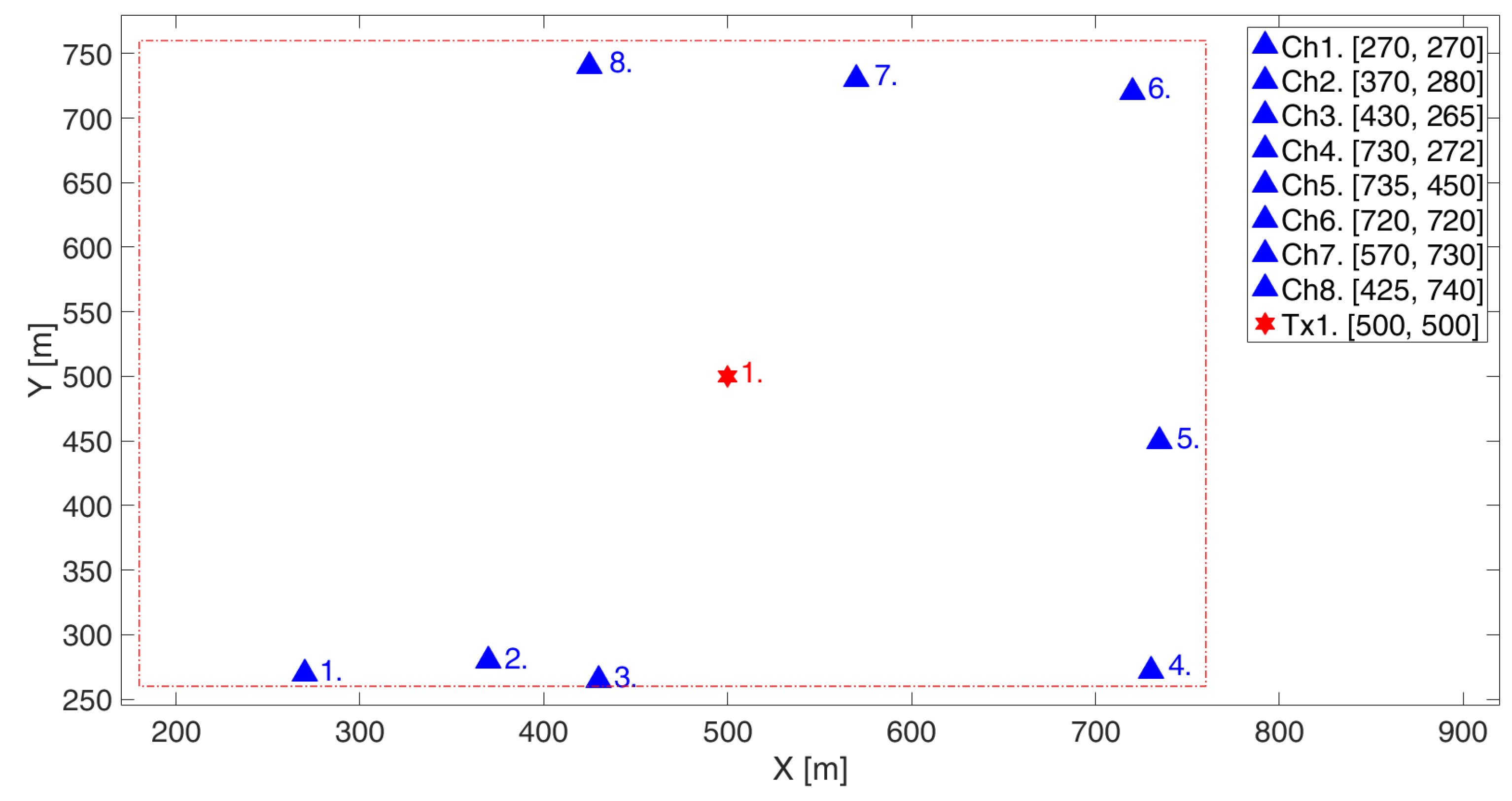
The advantages of the algorithm for the localization of impulse acoustic source are presented through qualitative and quantitative results. To demonstrate the qualitative results, a scenario with one and multiple sources was generated. The constellation of the microphone array and one source is given in Figure 2. The problem of outdoor localization is analyzed in a relatively small area (such as 580 × 500 m), for which the isotropicity of the meteo factors can be assumed. The positions of microphones in the eight-channel array are indicated by triangles, and the locations of the sources are shown by a star (in all figures). The legend gives the coordinates of each microphone and source in meters. The dashed line shows the region of interest within which the localization of acoustic sources is performed.

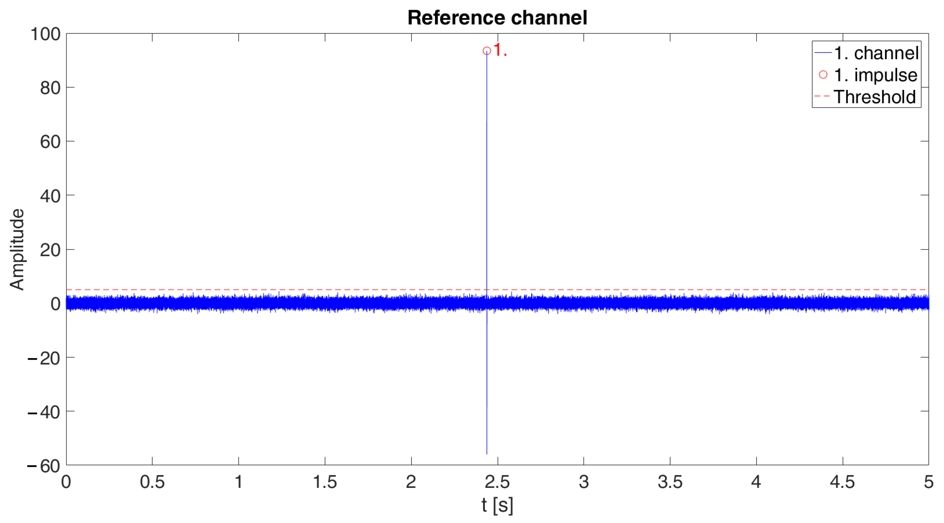
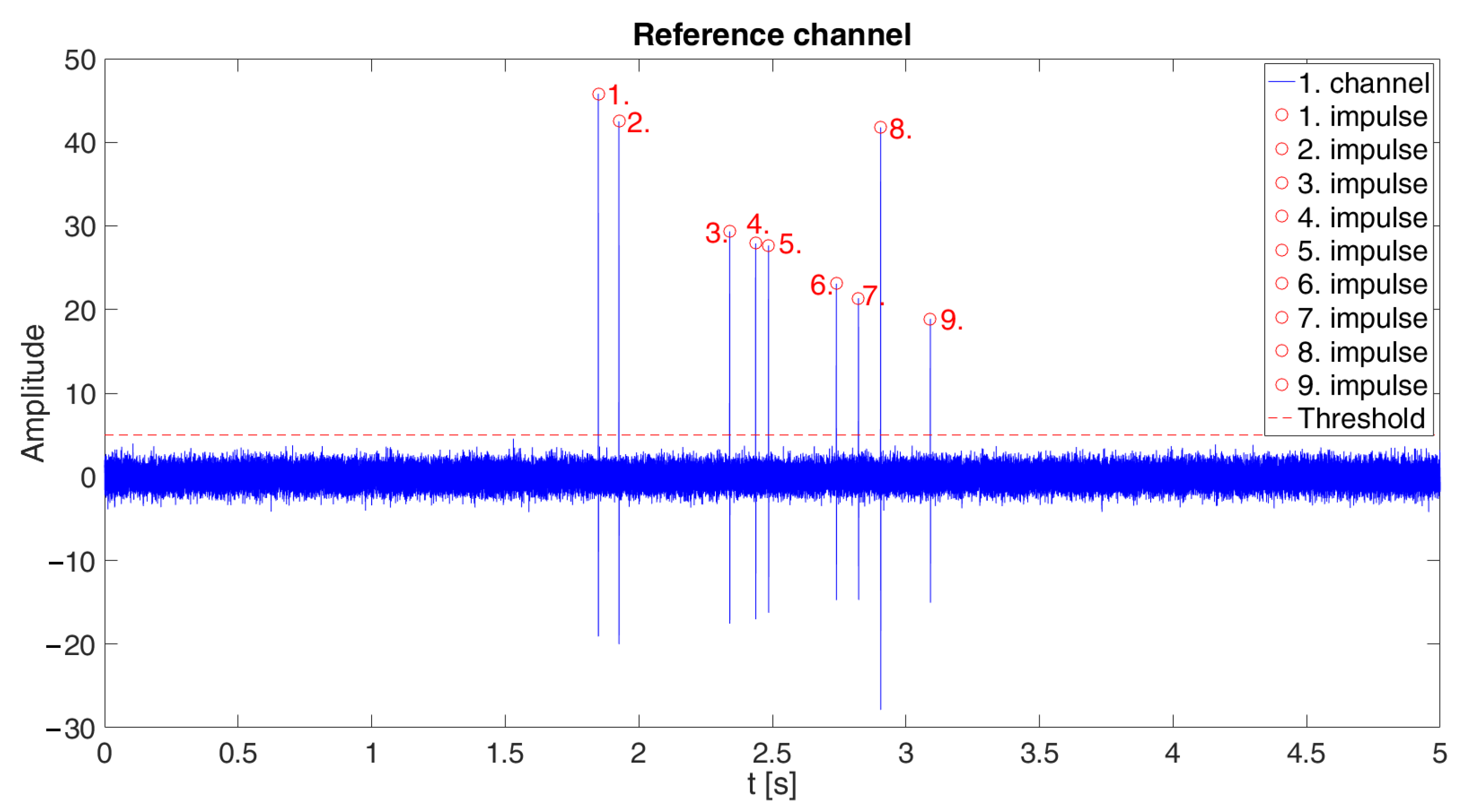
Simulated, simultaneous and time-synchronized signal acquisition is performed from a microphone array. The channel with number one was selected to be the reference, i.e., $p_{\mathrm{ref}}=1$, so the detection of received signal is performed on it, as shown in Figure 3.

The generated acoustic source impulse lasts 1 ms.

The simulations use the following meteorological parameters for modeling the propagation of the acoustic signal: air temperature $T=26{}^{\circ }\mathrm{C}$, relative humidity $h_r=20\%$ and ambient atmospheric pressure $p_a=101.13\mathrm{kPa}$.

Apart from the attenuation, additive white Gaussian noise (AWGN) of variance ${\sigma }_{\mathrm{n}}^2=1$ was added to the signal. Since useful signals are single impulses, their average power is not well defined because, by simply setting a longer observation interval, we would obtain a lower average signal power, even though it is the same signal. So, we used (as a parameter) the total energy of the impulse instead. Conversely, the energy of the noise is not well defined because, by simply setting a longer interval, we would obtain a higher noise energy. Therefore, we used the power spectral density (PSD) of the noise instead. So, the SNR is defined as $E_{\mathrm{I}}/P_{\mathrm{N}}$, the ratio of the impulse energy in the reference receiving channel, and the noise PSD in the same point. The noise variance (${\sigma }_{\mathrm{n}}^2=1$), the shape of the impulse (the waveform), and the chosen value of $E_{\mathrm{I}}/P_{\mathrm{N}}$ determine the amplitude of the impulse in Figure 3. The ratio value $E_{\mathrm{I}}/P_{\mathrm{N}}=70,000\left(48.45\mathrm{dB}\right)$ was set. 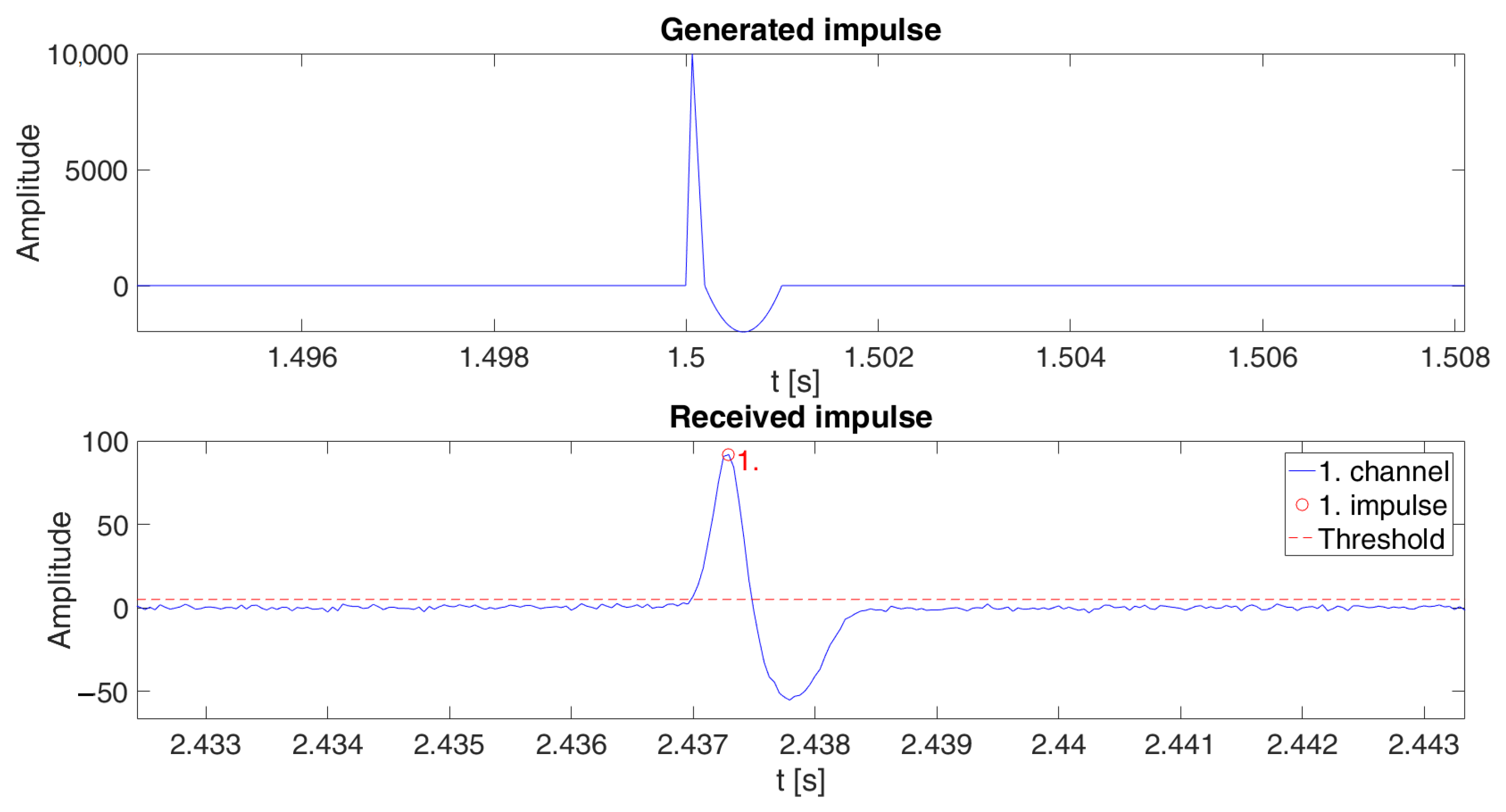Figure 4 shows the shape of the generated and received impulse of the acoustic signal. The influence of the attenuation on the impulse’s amplitude and shape is obvious.

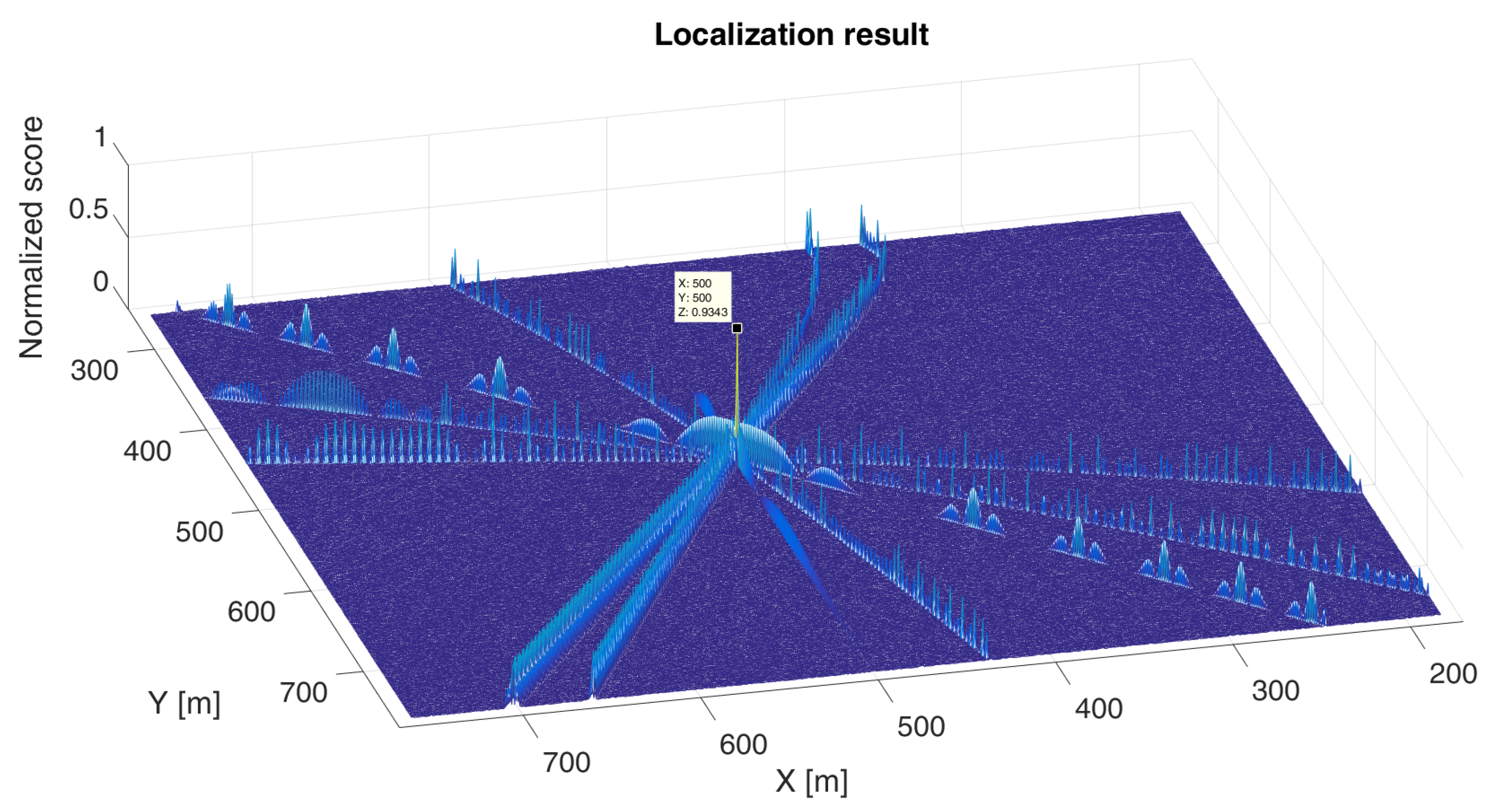
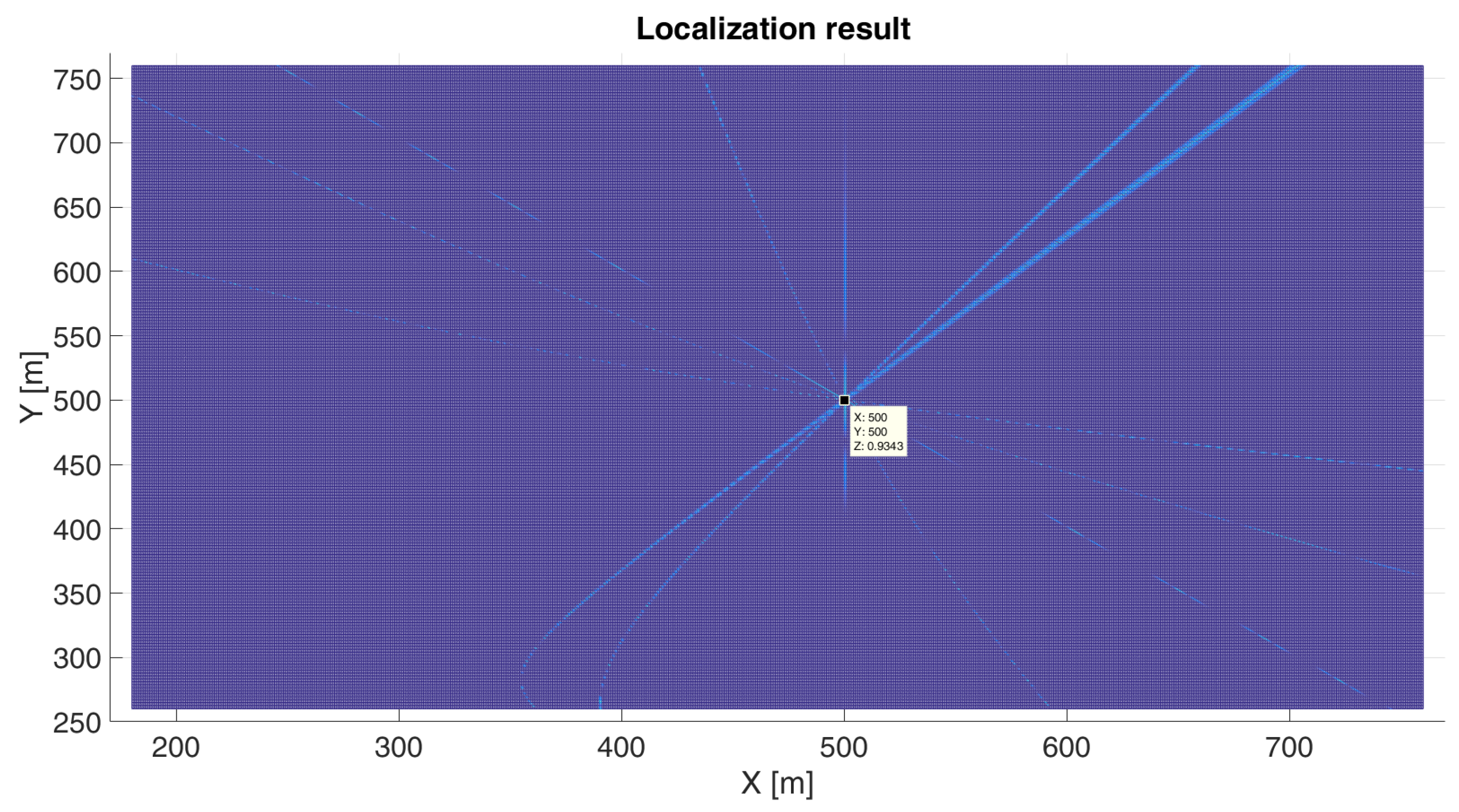
The results of localization and the normalized values of the criterion function are given in Figure 5 and Figure 6. The search resolution is 1 m on both axes. Figure 7 shows the localization results for the narrower spatial sector $1\times 1$ m around the actual location of the source in order to show the shape of the criterion function. The search resolution is 1 cm on both axes.

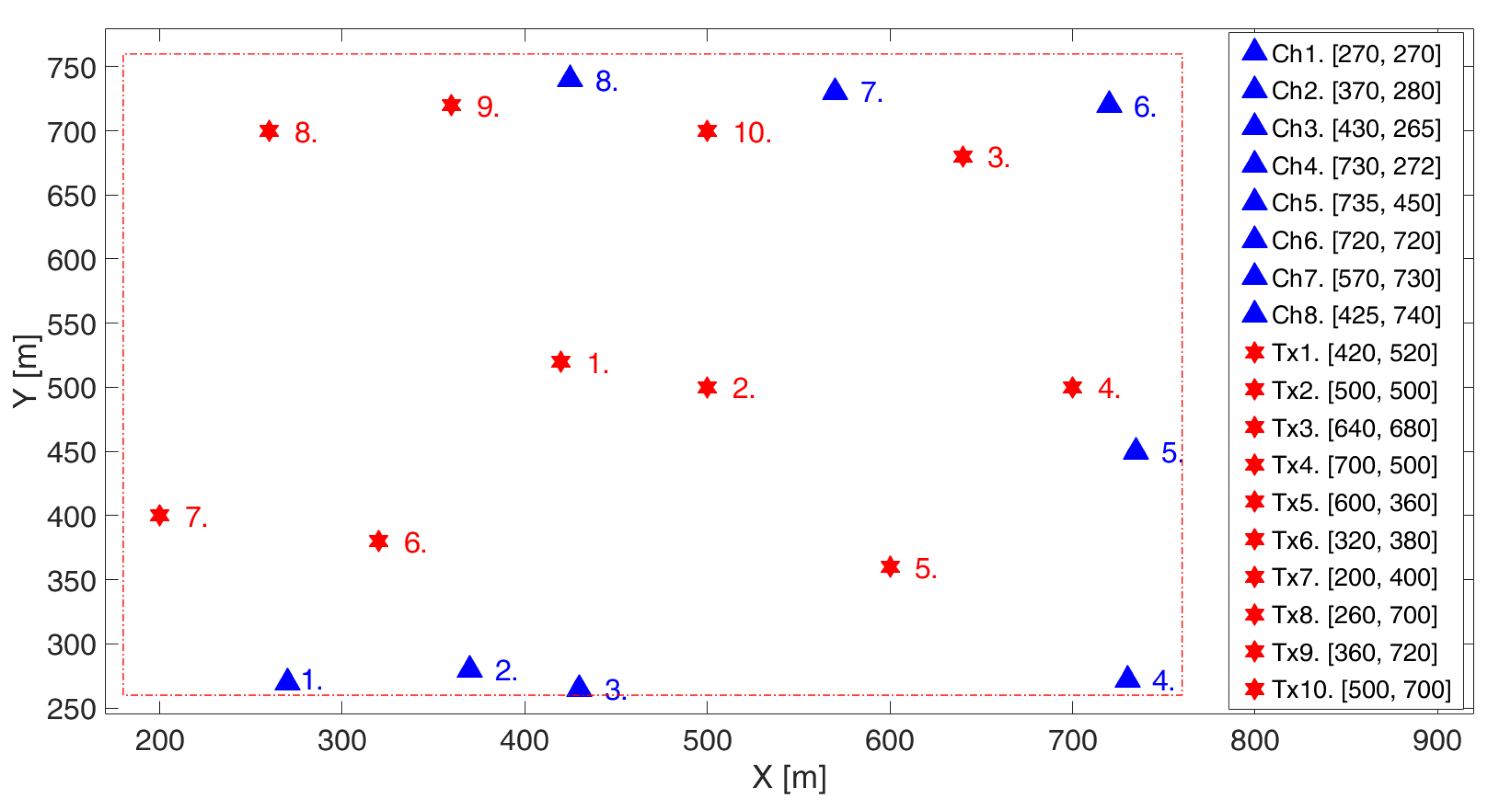
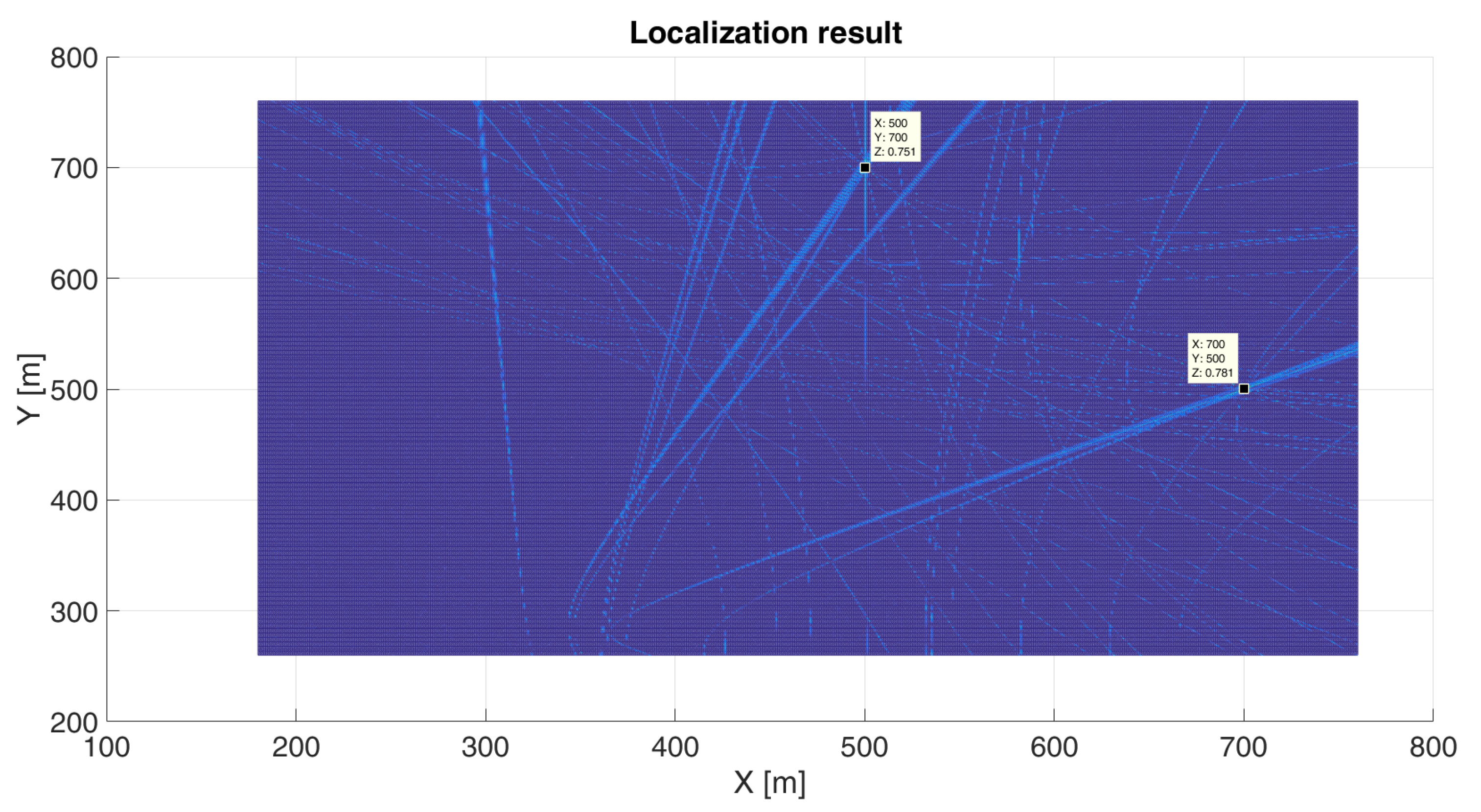
The constellation of the microphone array and 10 acoustic signal sources are given in Figure 8. This spatial arrangement of microphones in the microphone array and signal sources (simultaneously active sources) leads to an order permutation of the impulses on microphones. The first microphone is declared the reference channel. Acoustic sources that are localized are detected and selected in the reference channel. The order of the acoustic signals (given by the indices of their sources) arriving in the reference channel is as follows: 6, 7, 1, 2, 5, 8, 9. Then, the impulses from Tx10 and Tx4 arrive simultaneously, and, finally, the impulse from Tx3 arrives last. These correspond to the detected impulses from the first to the 9-th respectively (Figure 9). In addition to the signals order permutation on the microphones, the acoustic signals of the 10-th and 4-th sources completely overlap and superimpose in the reference channel. Because of that, 9 impulse acoustic signal sources were detected in the reference channel instead of the generated 10.

All of the acoustic sources are of the impulse type and have identical parameters. Other parameters in the simulation are identical as above.

Figure 10 shows the normalized values of the criterion function. These values are the localization results in a scenario with multiple impulse acoustic sources. The algorithm successfully localized all 10 sources, despite detecting only 9 impulses in the reference channel, and overcame the problems of the permutation of the order of signal arrivals on the microphone array. Additionally, the algorithm successfully separated two time-overlapping impulses of acoustic sources, 4-th (500,700) and 10-th (700,500). The search grid resolution is 1 m on both axes.

Figure 11 and Figure 12 depict the localization result of the 8-th impulse. The result shows that the two acoustic sources overlapping in time were successfully separated.

The RMS deviation of the estimated acoustic impulse source location from the true location is obtained by simulations and quantitatively describes the performance of the algorithm.

For the purpose of presenting the quantitative results, the scenario with one acoustic impulse source (already described above) with the same meteorological parameters was used. Additionally, the spatial sector was reduced to $1\times 1$ m with an initial resolution of 10 cm along the x- and y axes. The number of points is 11 along each of the axes (x and y). At the beginning of each localization in the region of interest, a grid displacement is performed so that the actual location of the acoustic source is not on the grid (to make the simulations more realistic). After a location estimate is obtained, the span of the grid is reduced by a factor of two along the x and y axis. The number of grid points remains the same, $11\times 11$. The new grid is centered at the estimate obtained with the previous (larger) grid. After that, the localization process is restarted. This grid size reduction was performed three times, so the estimate after the third reduction is considered the final estimate of the impulse acoustic source location. This is considered a single localization cycle. At the beginning of the cycle, the noise is added according to the selected value of the ratio $E_{\mathrm{I}}/P_{\mathrm{N}}$.

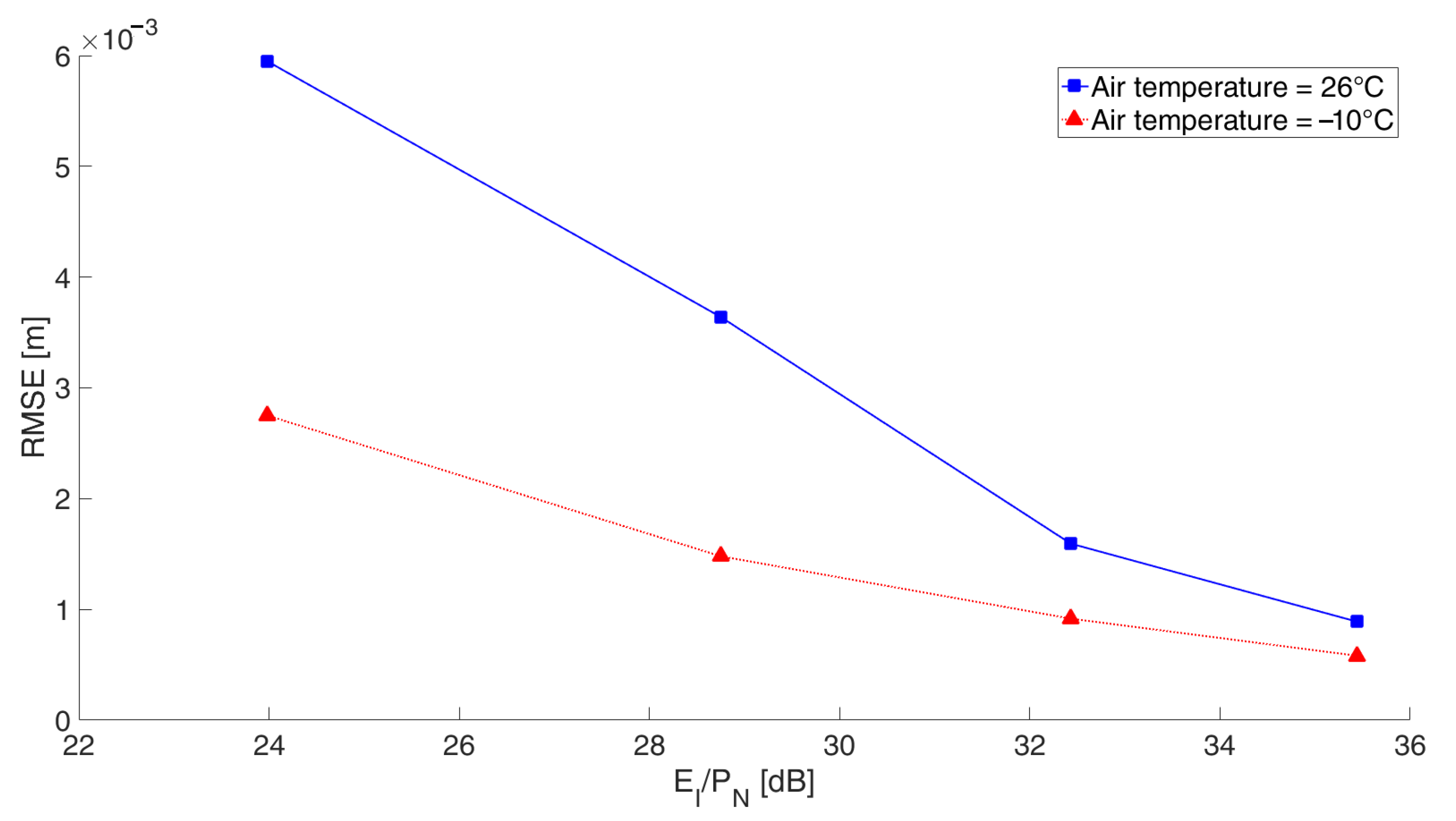
Figure 13 shows the value of the Root Mean Square Error (RMSE) depending on the value of the ratio $E_{\mathrm{I}}/P_{\mathrm{N}}$ for different temperatures ($26{}^{\circ }\mathrm{C}$ and $-10{}^{\circ }\mathrm{C}$) in order to see the influence of temperature as the dominant effect. For each set value $E_{\mathrm{I}}/P_{\mathrm{N}}$ from Figure 13, 100 localization cycles were performed. Note that, in the scenario in Figure 2, for ratios $E_{\mathrm{I}}/P_{\mathrm{N}}$ lower than 23 dB, the impulse in the referent channel is no longer detectable. The numerical results confirm the theoretical predictions according to [35].

Simulation results show that for the same values of $E_{\mathrm{I}}/P_{\mathrm{N}}$ on the reference microphone, there are differences in the RMSE values at different temperatures. This is due to the fact that at different temperatures, the propagation speed of the acoustic signal changes, and the attenuation during the propagation changes, which affects the shape, the duration and the attenuation of the signal on other microphones in the distributed microphone array.

5. Conclusions

The proposed method provides direct (i.e., one-step) localization of multiple impulse acoustic sources in an outdoor environment, so the association problem, which is typical for two-step localization methods, does not exist. The solution to this problem is inherently included in the proposed direct localization method. Meteorological factors (such as air temperature, relative humidity, and ambient atmospheric pressure), which affect impulse duration, shape, and amplitude, are included in the signal model of the multiple impulse acoustic scenario. Furthermore, in the proposed method, direct localization is performed impulse by impulse, so the observation intervals used for localization are limited by the duration of impulses used for localization. In a typical multiple impulse acoustic scenario, observation intervals may or may not overlap in time and, due to the meteorological effects, they are not of the same duration.

The criterion function of the proposed direct localization method is formulated as a normalized measure of collinearity between the vector with chained impulses in the observation intervals at different microphones and a feature vector constructed by mathematical modeling. This function is calculated at given grid points in the space. The maximum of the criterion function corresponds to the impulse source locations.

The performance of the proposed method is illustrated by the simulations for single and multiple impulse sources.

The results provided by a single source scenario with nonuniform eight-microphone array distributed in the area of approximately $580\times 500$ m prove that the localization accuracy of the order of 1 cm can be achieved for a signal-to-noise ratio of 48.45 dB defined as the ratio of the impulse energy in the reference receiving channel and the noise power spectral density (PSD) in the same point. Furthermore, in the criterion function, some sidelobes are visible, which are specific for the microphone array geometry.

The multiple impulse acoustic scenario with 10 sources is simulated. In this scenario, the impulses of 2 sources fully overlap in time on the referent microphone, but in spite of that, all 10 sources are localized. One of the significant advantages of the new method is the possibility of localization of two impulse acoustic sources at different positions, which completely overlap in time at the reference (or other) microphone.

The results of quantitative analysis show that a RMS of localization errors for the above single signal scenario that is better than 6 mm can be achieved for $E_{\mathrm{I}}/P_{\mathrm{N}}$ smaller than 24 dB.

Presented results show that centimeter localization accuracy can be achieved.

In the proposed signal model, it is assumed that receiving microphone channels are perfectly time synchronized and the microphone positions are known. In real situations, there are many factors which degrade the localization performance of the proposed method, such as imperfect time synchronization, uncertainty in the microphone positions, meteo factors, multipath, non-line of sight propagation, etc. The wind is also an important factor, and taking it into account will be the focus of future research.

The subject of the future research will be the analysis of theoretical localization limitations for the given system and signal model, and the experimental verification of the proposed method in order to see what is the gap between the theoretical and the experimental performance metrics.

The proposed algorithm for the localization implicitly starts from the assumption that microphones should have a linear phase characteristic in the frequency range used for the localization (12 kHz in the specific case) and have omnidirectional characteristics. Additionally, for the acquisition of acoustic signals, 24 bit A/D converters with a sampling frequency above 24 kHz are commercially available. So, the microphone choice and A/D conversion do not represent a technological barrier.

From the practical point of view, time synchronization of distributed microphones can be provided by the use of PPS signal (one pulse per second) of the GPS. By using the GPS technology, it is possible to ensure that the time differences of the front edges of the PPS signal at different locations are of the order of 20 ns. By using GPS synchronized oscillators, it is possible to ensure the stability of local oscillators (from which clocks for A/D conversion are generated) of order ${10}^{-8}$. So, the time synchronization of A/D conversion in distributed microphones does not represent a technological barrier for the implementation of the proposed localization method. All this indicates that we could verify it experimentally in the future.

Feature vector used in the criterion function of the proposed localization algorithm is constructed by mathematical modeling for a given class of impulse sources, so it may be possible to develop a system for the joint localization and identification of acoustic impulse sources. That will be a subject of the authors’ future research.