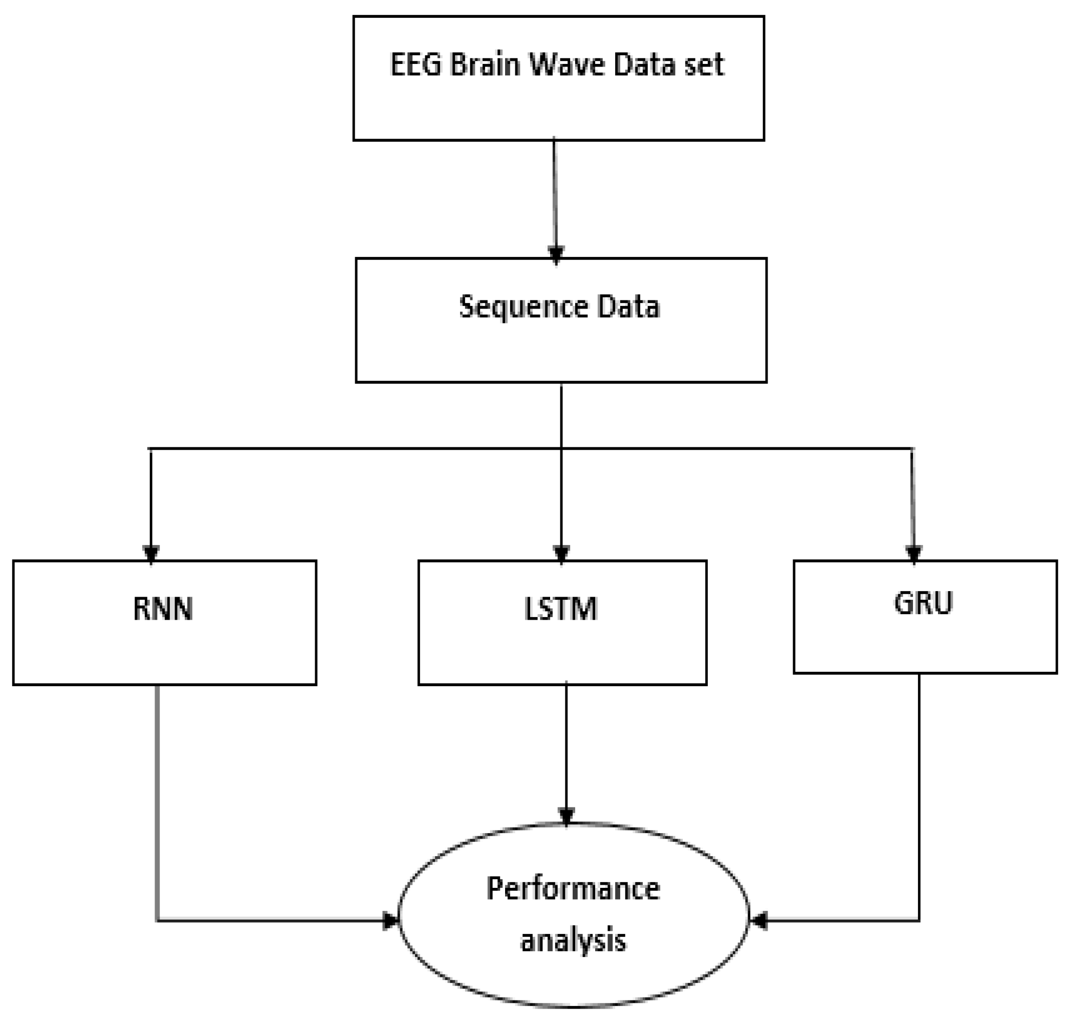
Figure 1.
EEG-based emotion recognition.
Figure 1.
EEG-based emotion recognition.
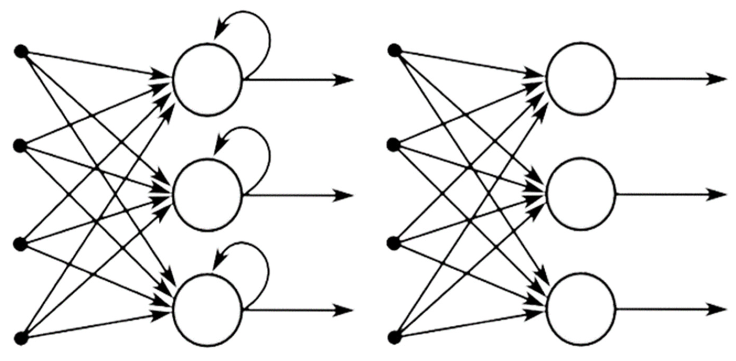
Figure 2.
Recurrent neural network and feed-forward neural network.
Figure 2.
Recurrent neural network and feed-forward neural network.
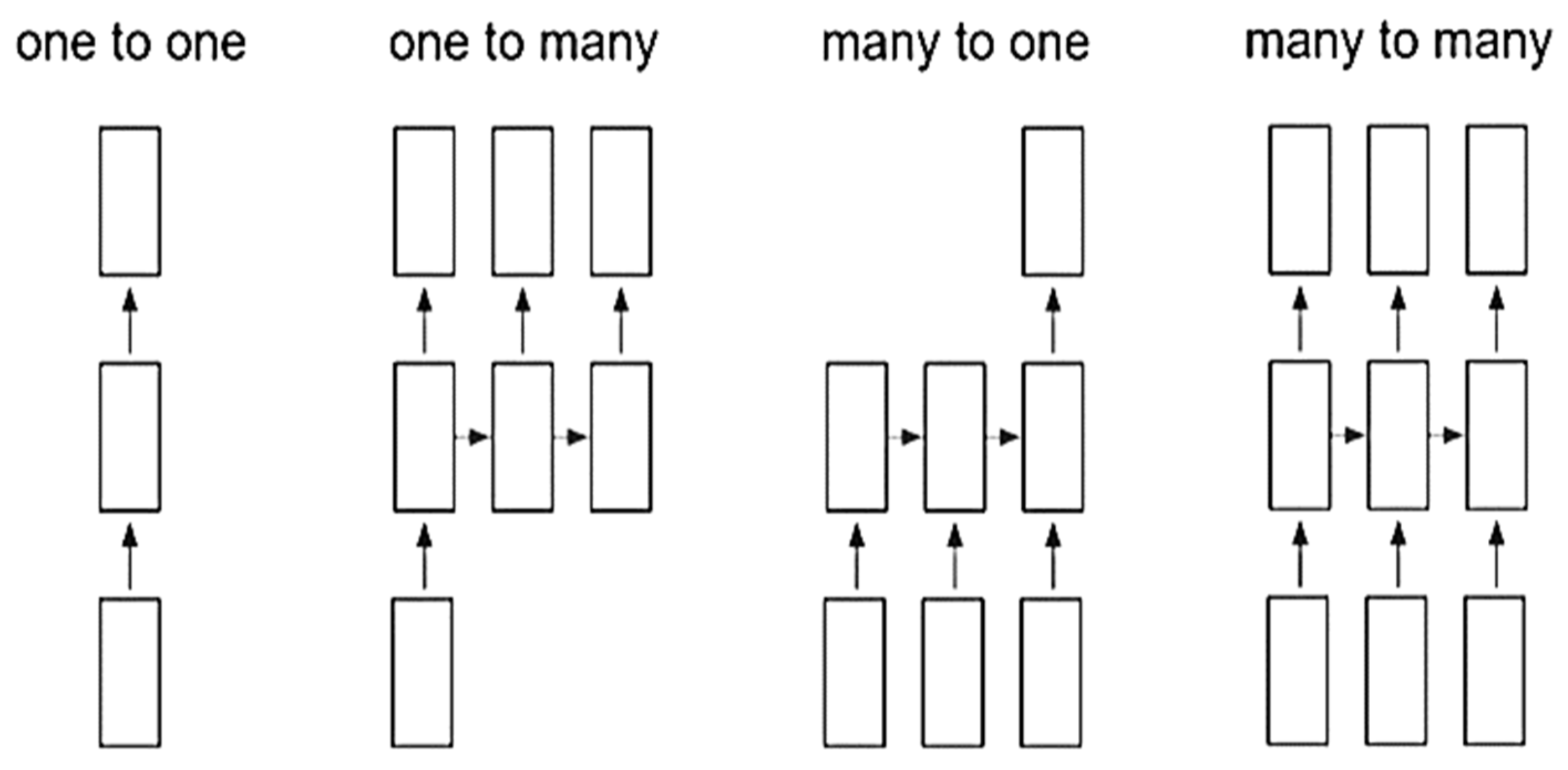
Figure 3.
Different types of RNN.
Figure 3.
Different types of RNN.
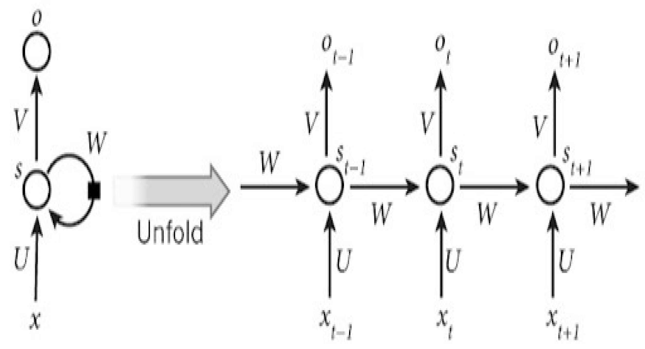
Figure 4.
The simple RNN (recurrent neural network) model.
Figure 4.
The simple RNN (recurrent neural network) model.
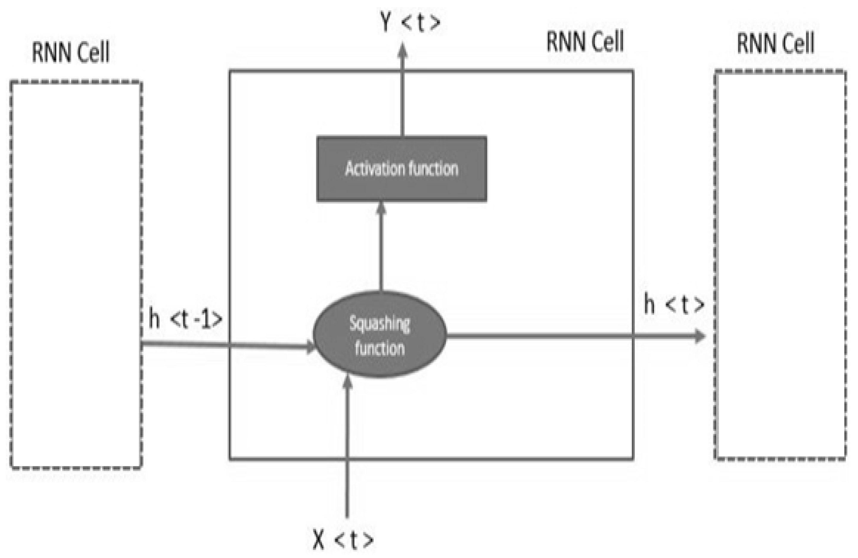
Figure 5.
Working of the recurrent neural network.
Figure 5.
Working of the recurrent neural network.
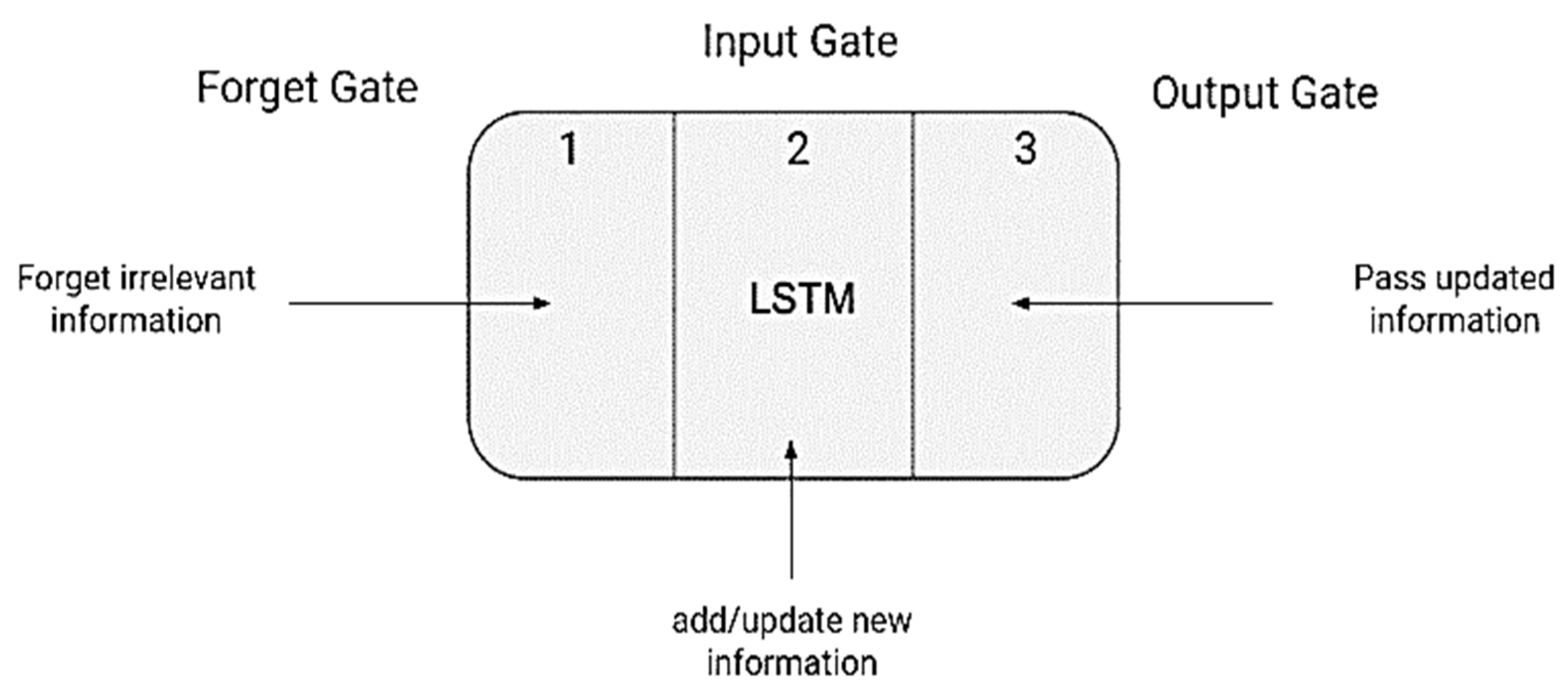
Figure 6.
LSTM cell with gates.
Figure 6.
LSTM cell with gates.
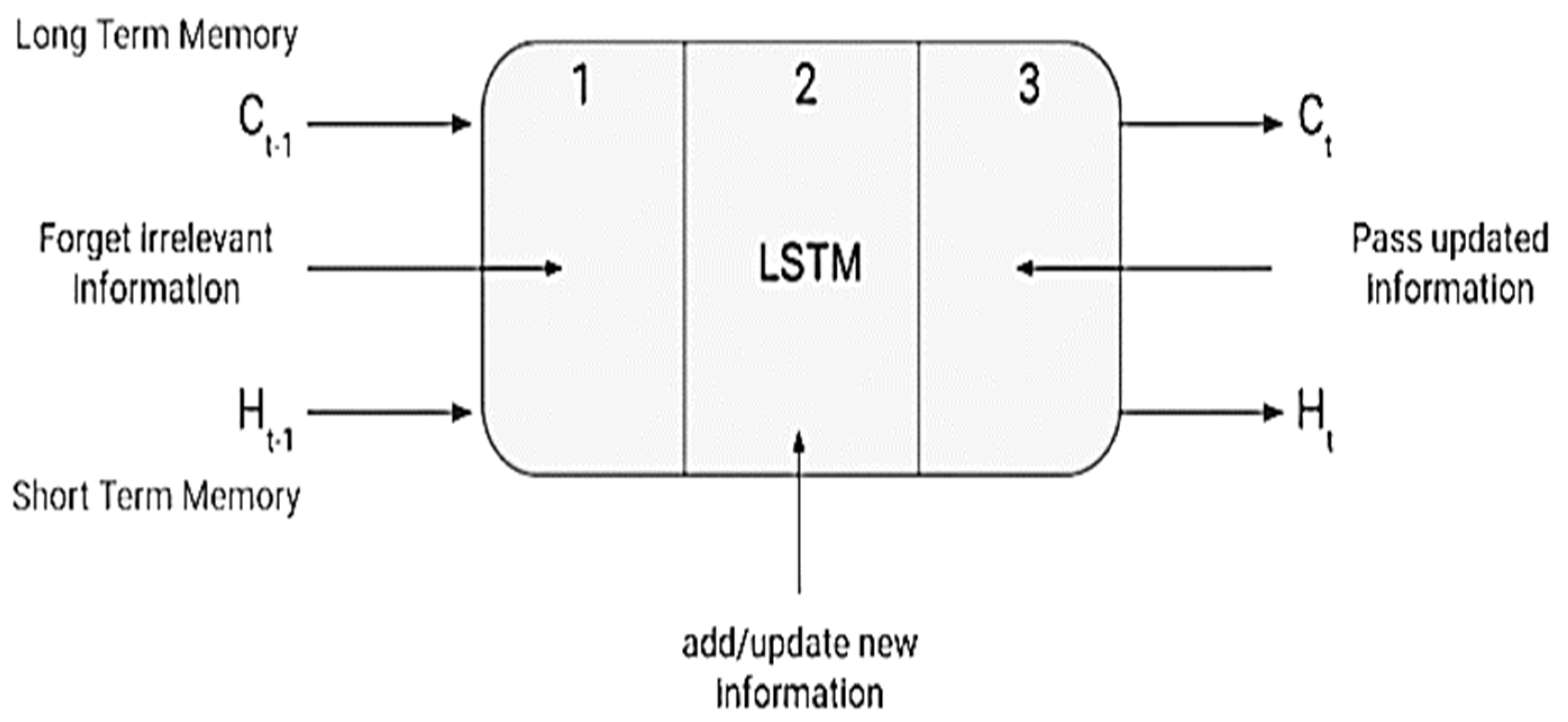
Figure 7.
LSTM cell with hidden and cell states.
Figure 7.
LSTM cell with hidden and cell states.
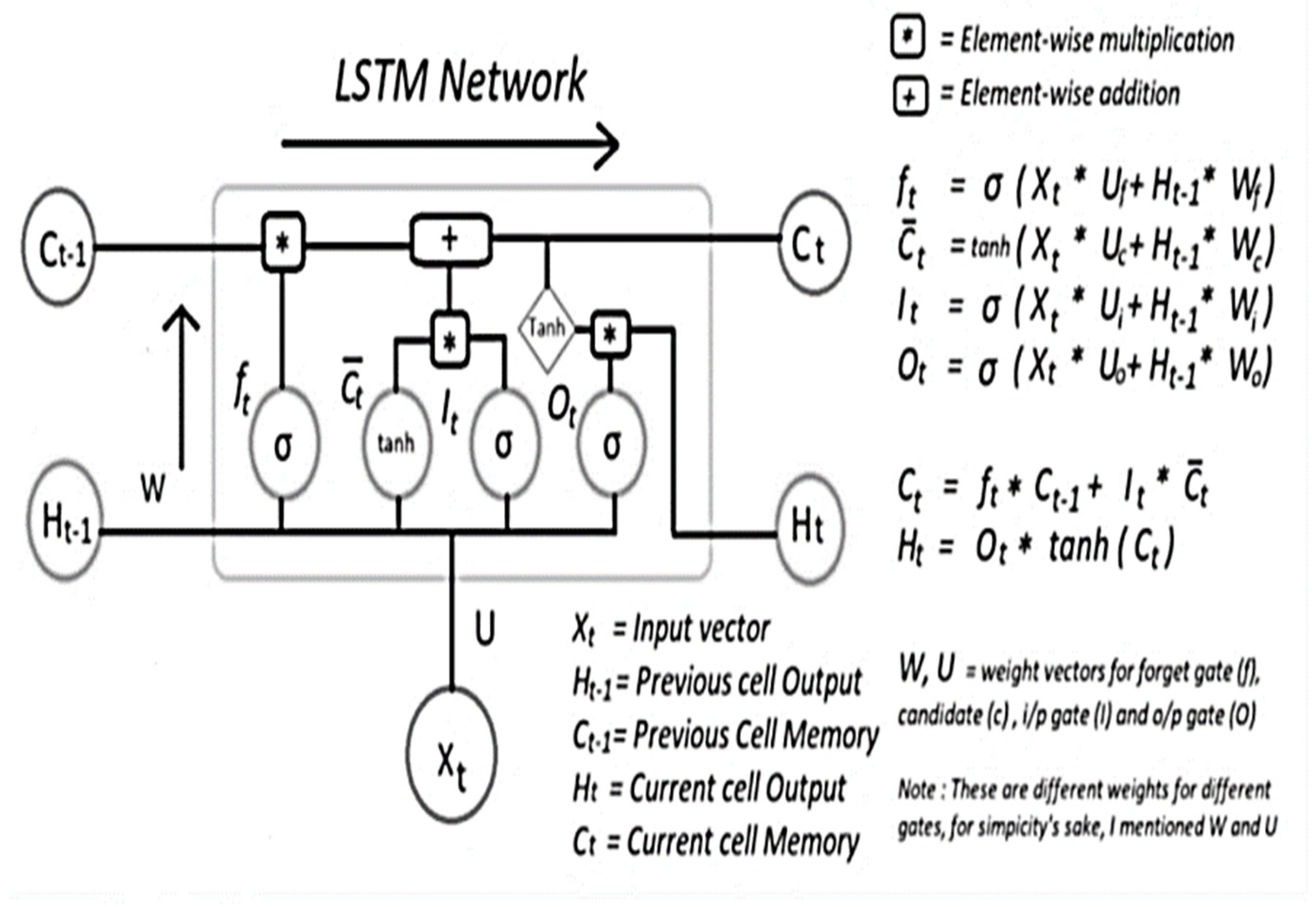
Figure 8.
Internal Working of LSTM cell.
Figure 8.
Internal Working of LSTM cell.
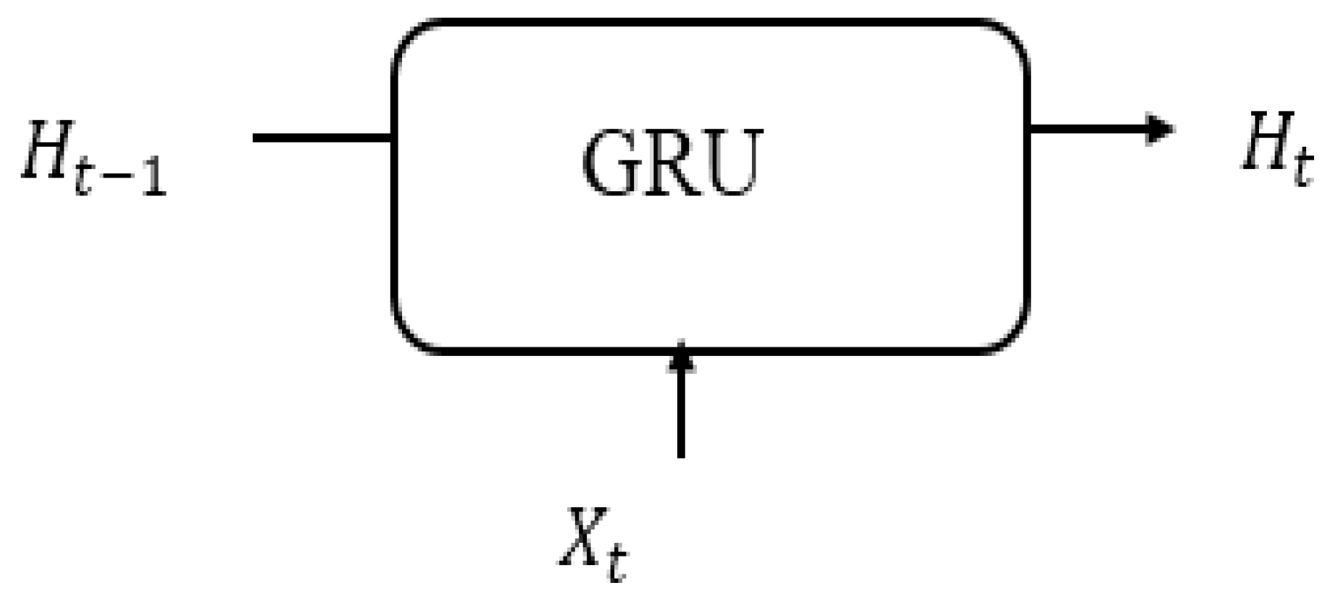
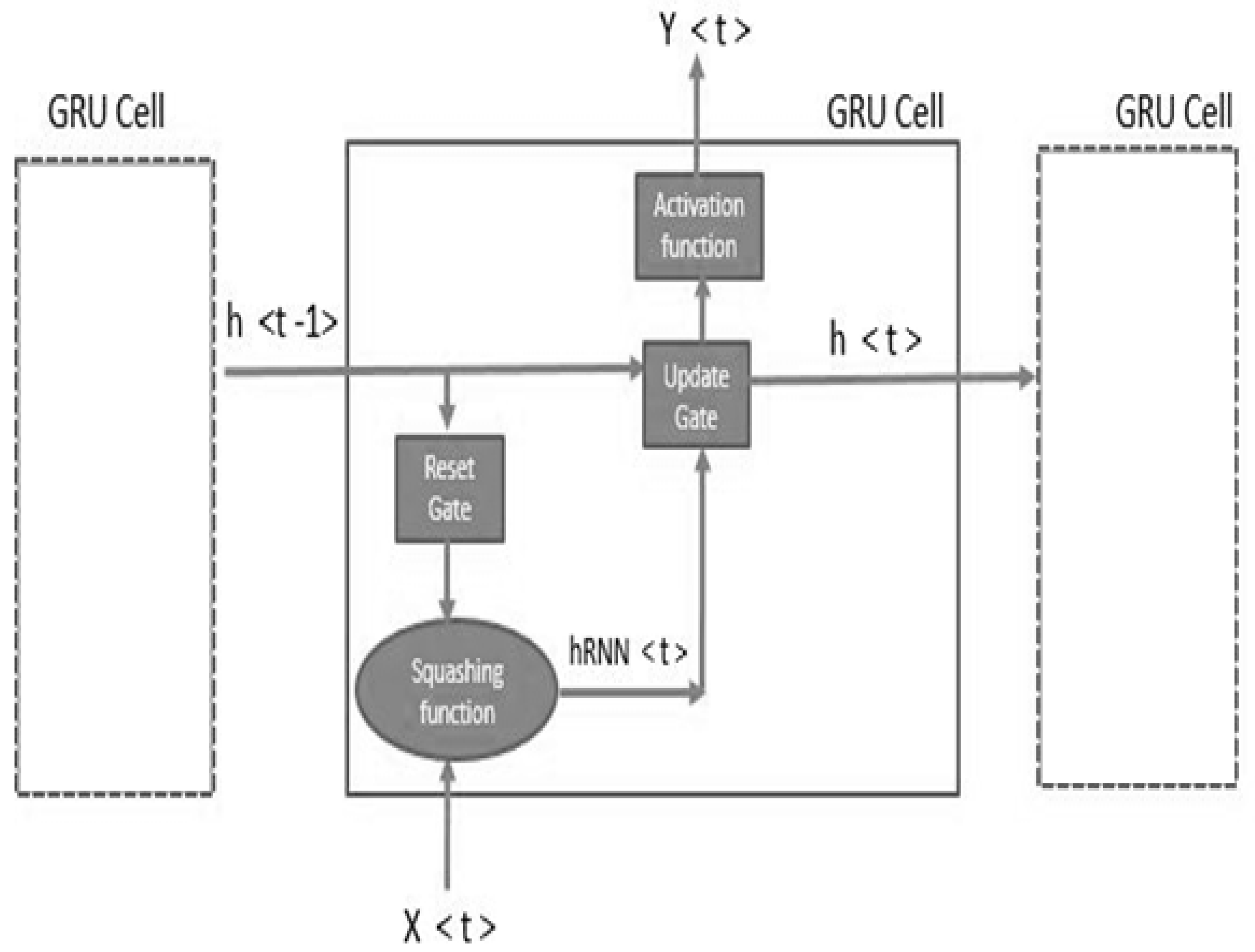
Figure 10.
Function of gated recurrent network.
Figure 10.
Function of gated recurrent network.
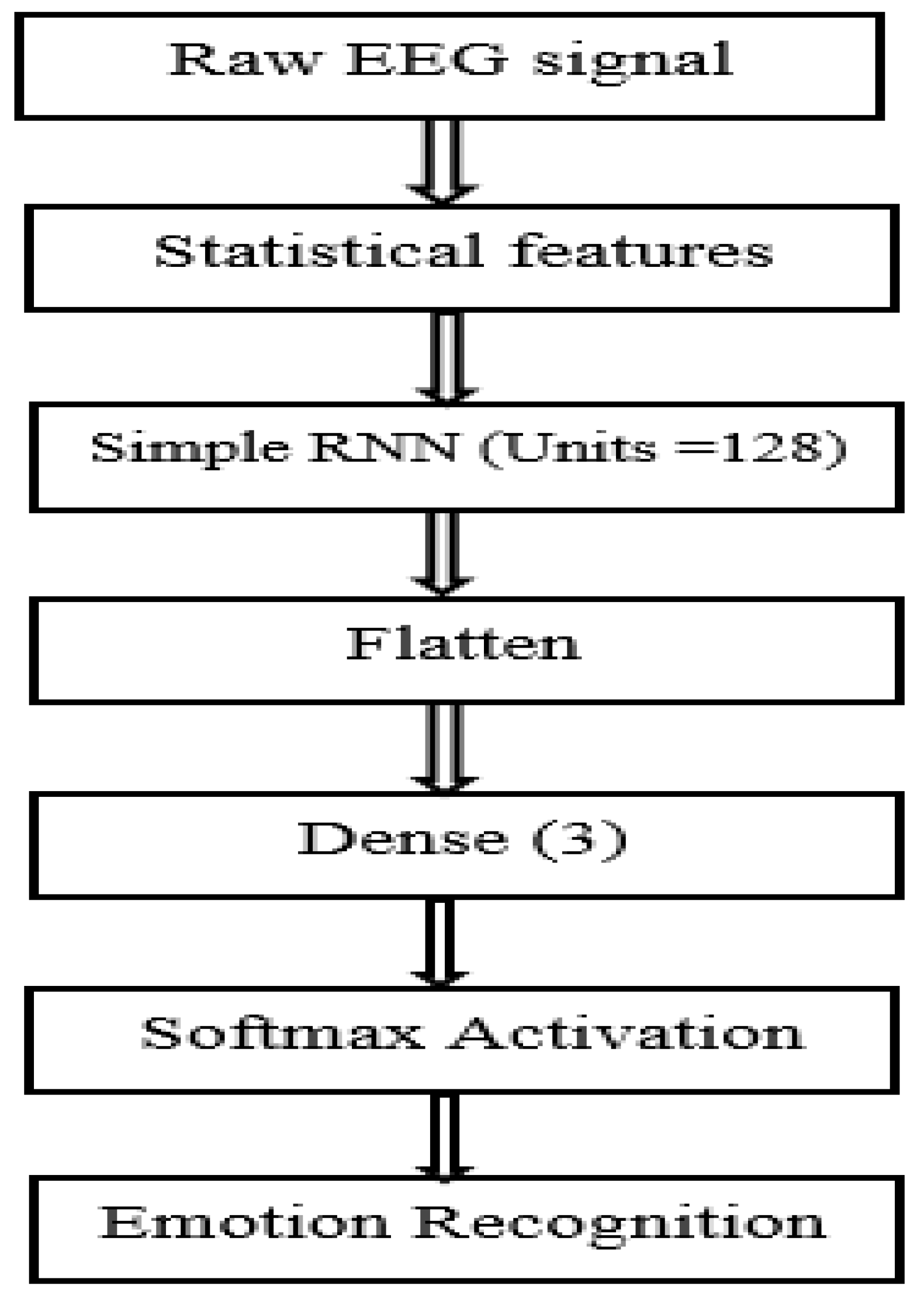
Figure 11.
Detailed RNN model.
Figure 11.
Detailed RNN model.
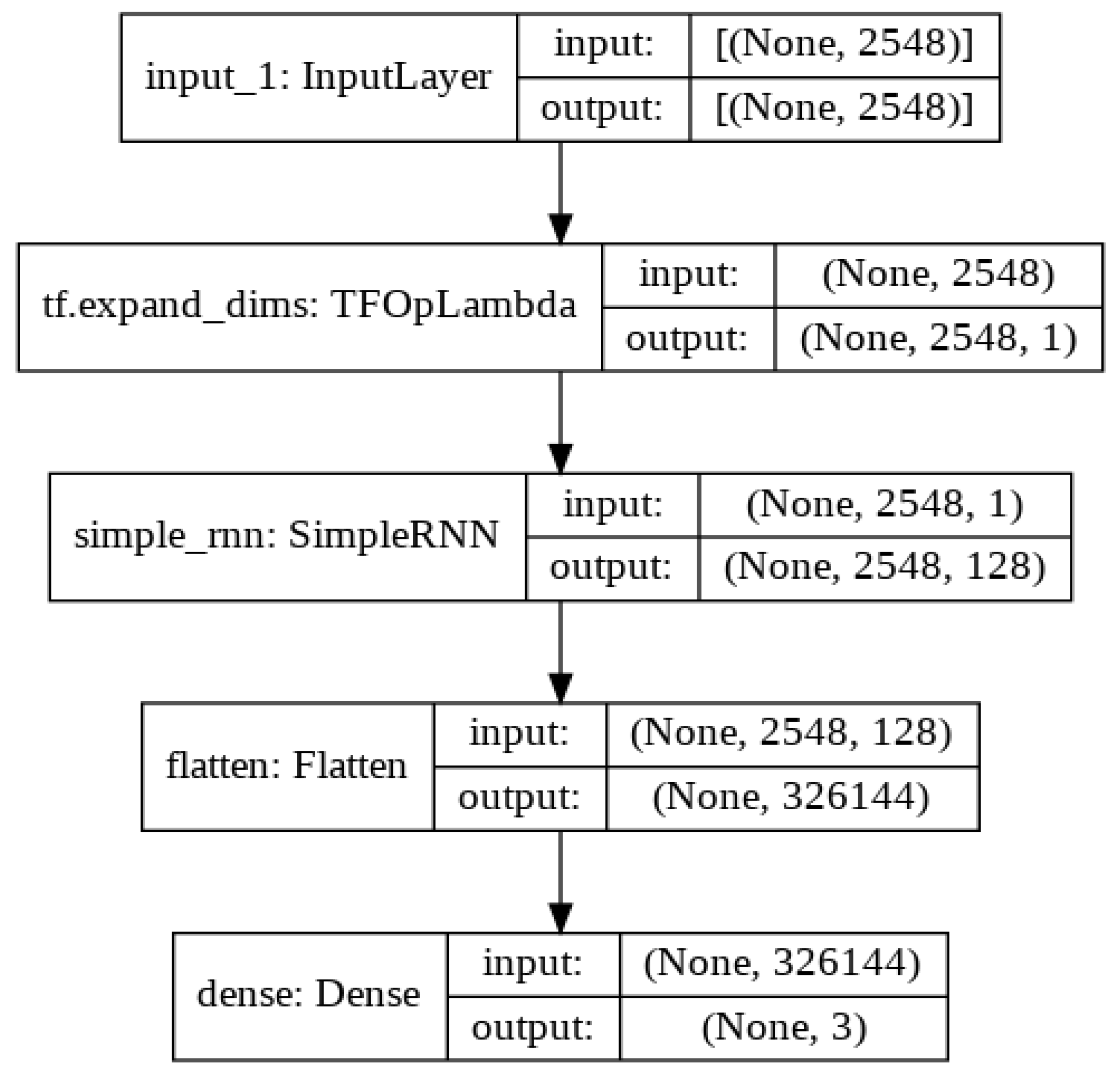
Figure 12.
Detailed RNN architecture with input and output vector shapes.
Figure 12.
Detailed RNN architecture with input and output vector shapes.
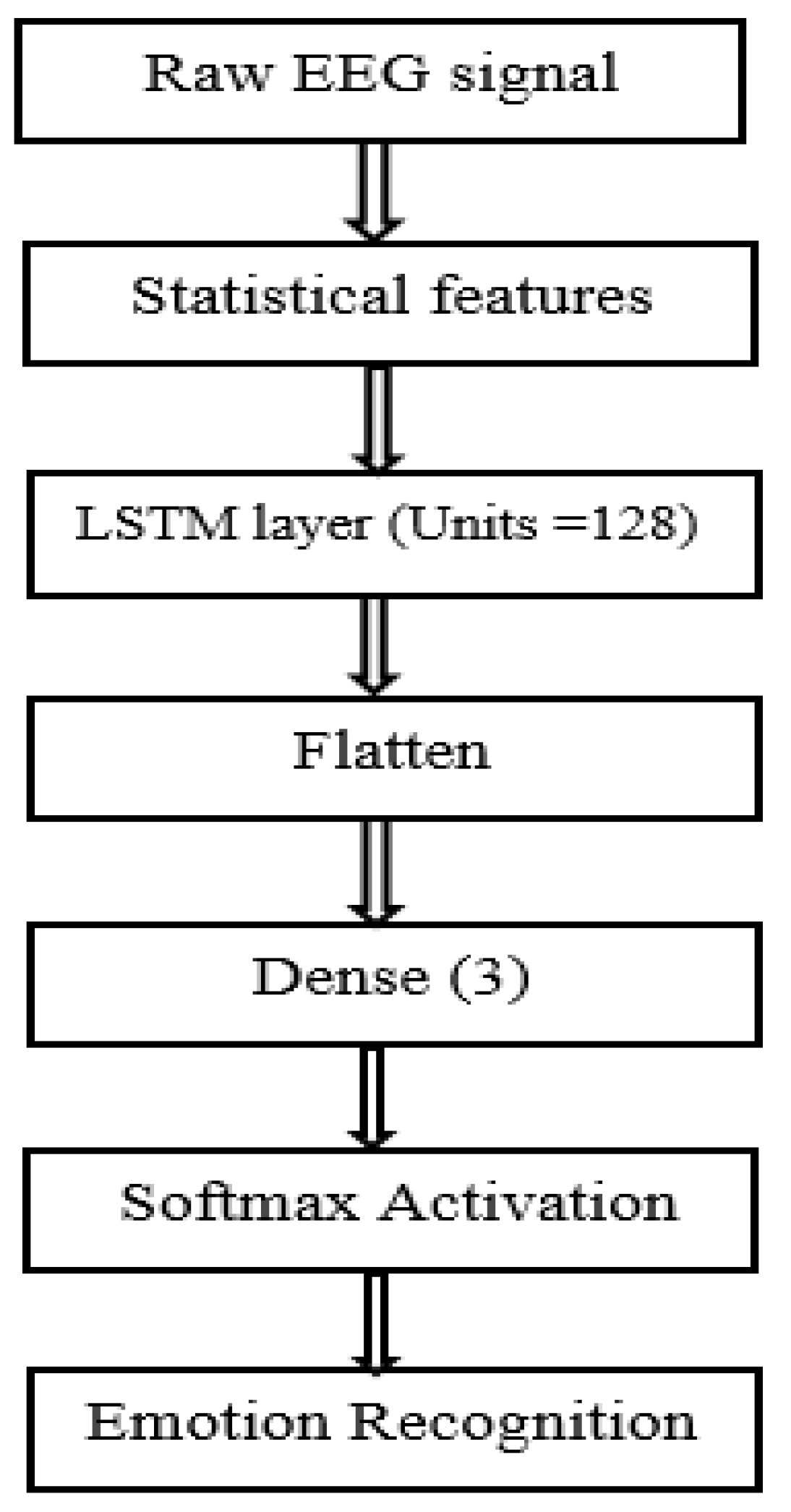
Figure 13.
Detailed LSTM model.
Figure 13.
Detailed LSTM model.
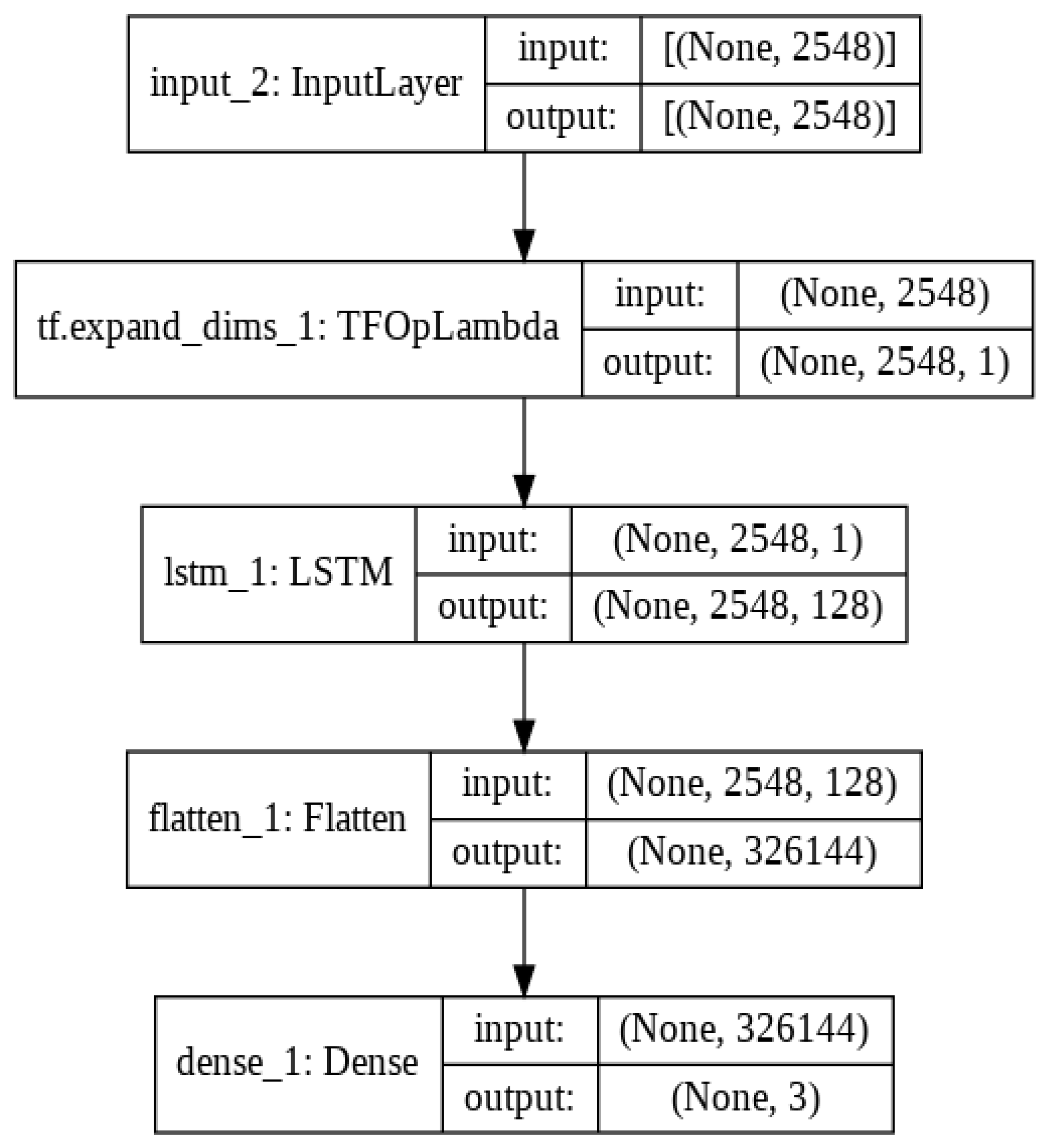
Figure 14.
Detailed LSTM architecture with input and output vector shapes.
Figure 14.
Detailed LSTM architecture with input and output vector shapes.
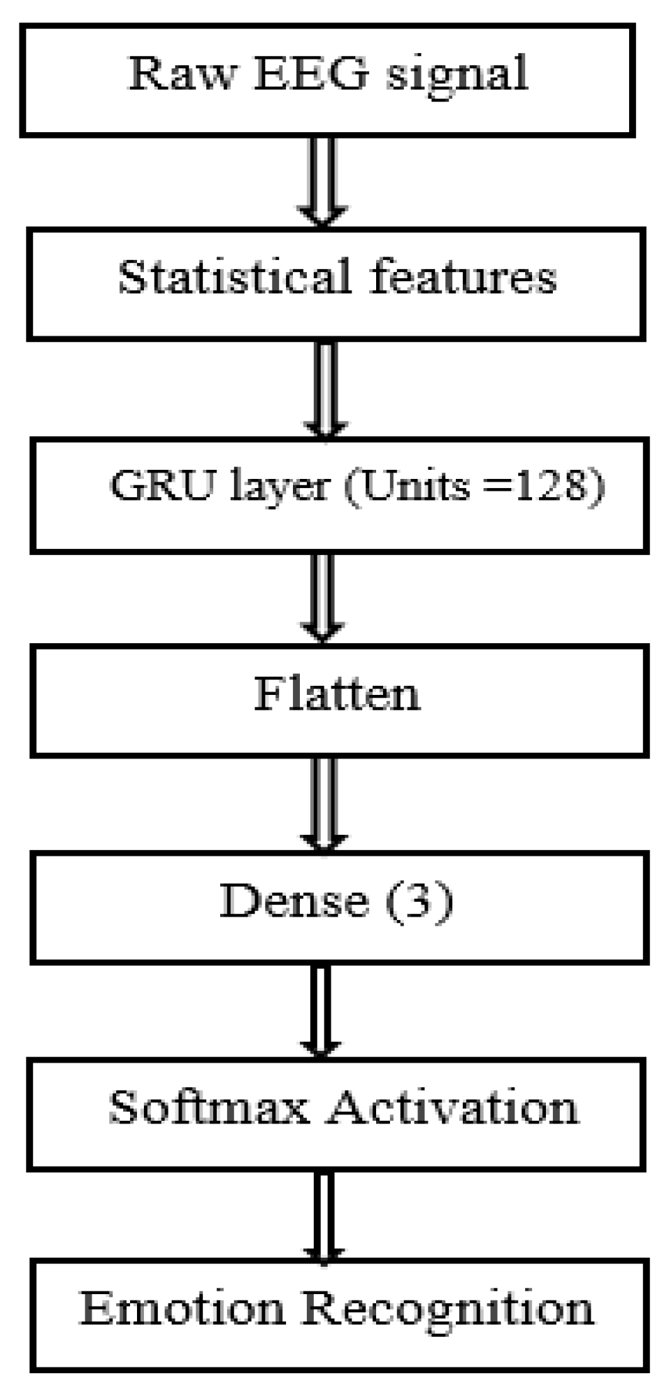
Figure 15.
Detailed GRU model.
Figure 15.
Detailed GRU model.
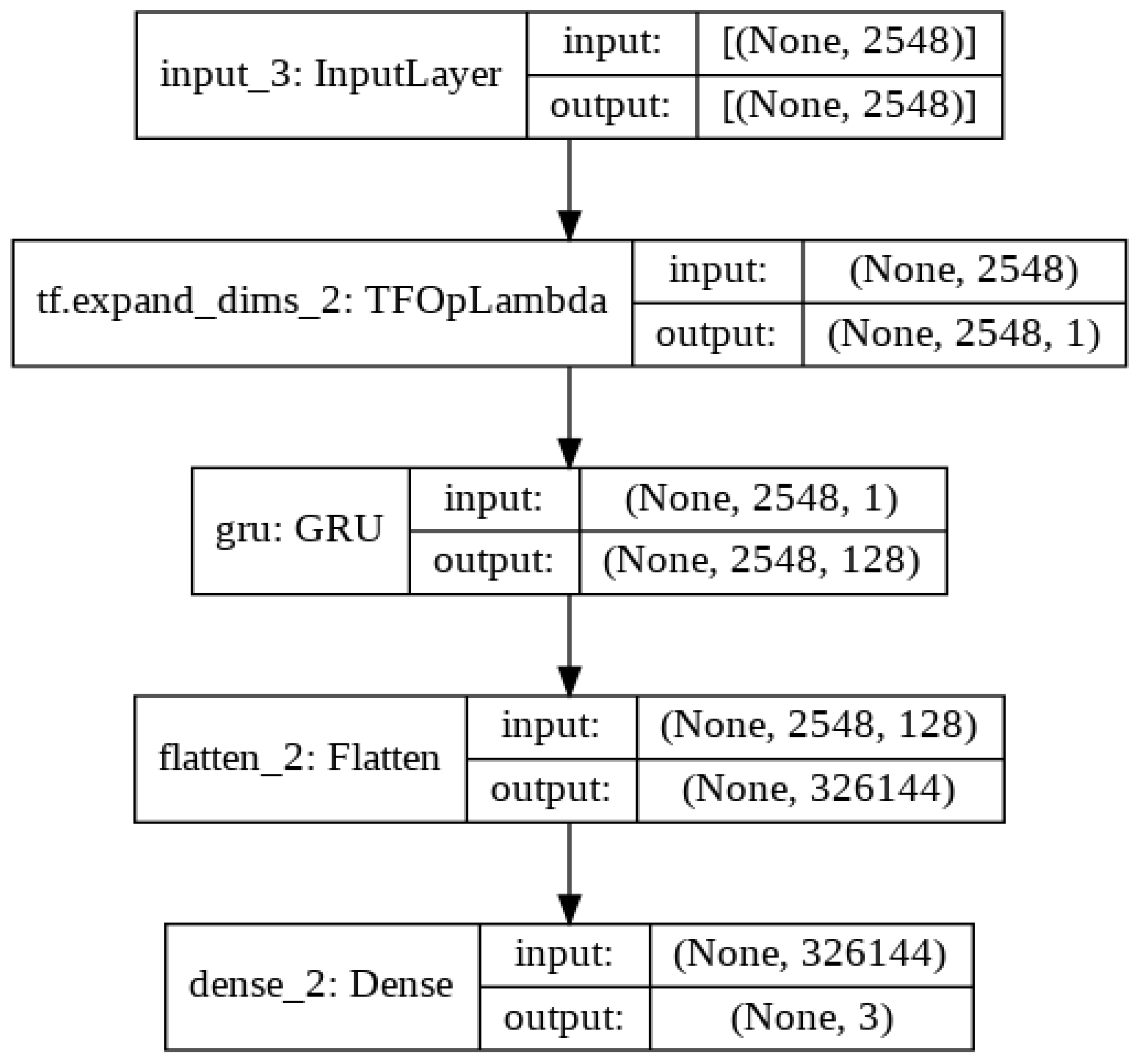
Figure 16.
Detailed GRU architecture with input and output vector shapes.
Figure 16.
Detailed GRU architecture with input and output vector shapes.
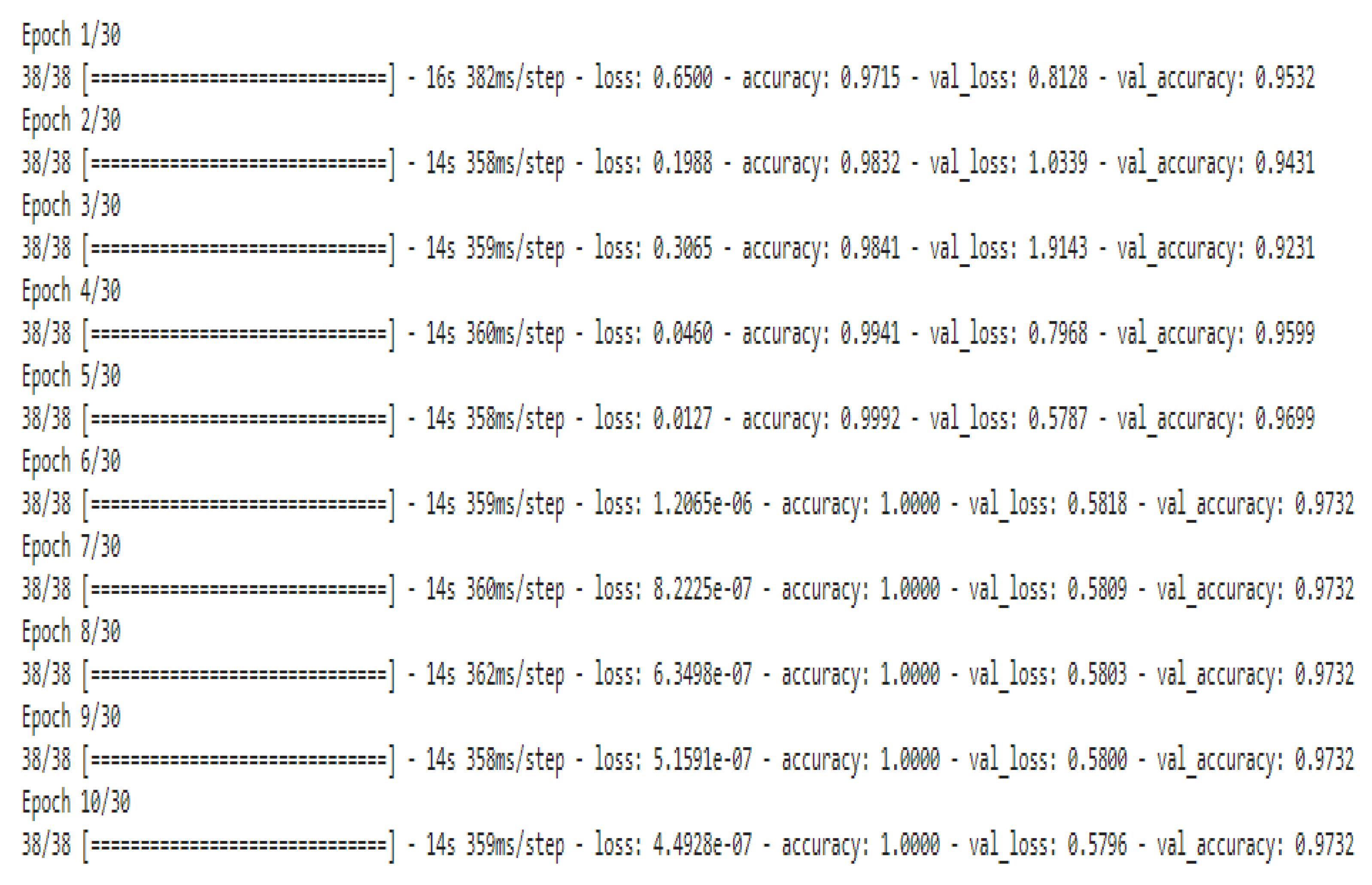
Figure 17.
Fitting results by using the RNN architecture.
Figure 17.
Fitting results by using the RNN architecture.
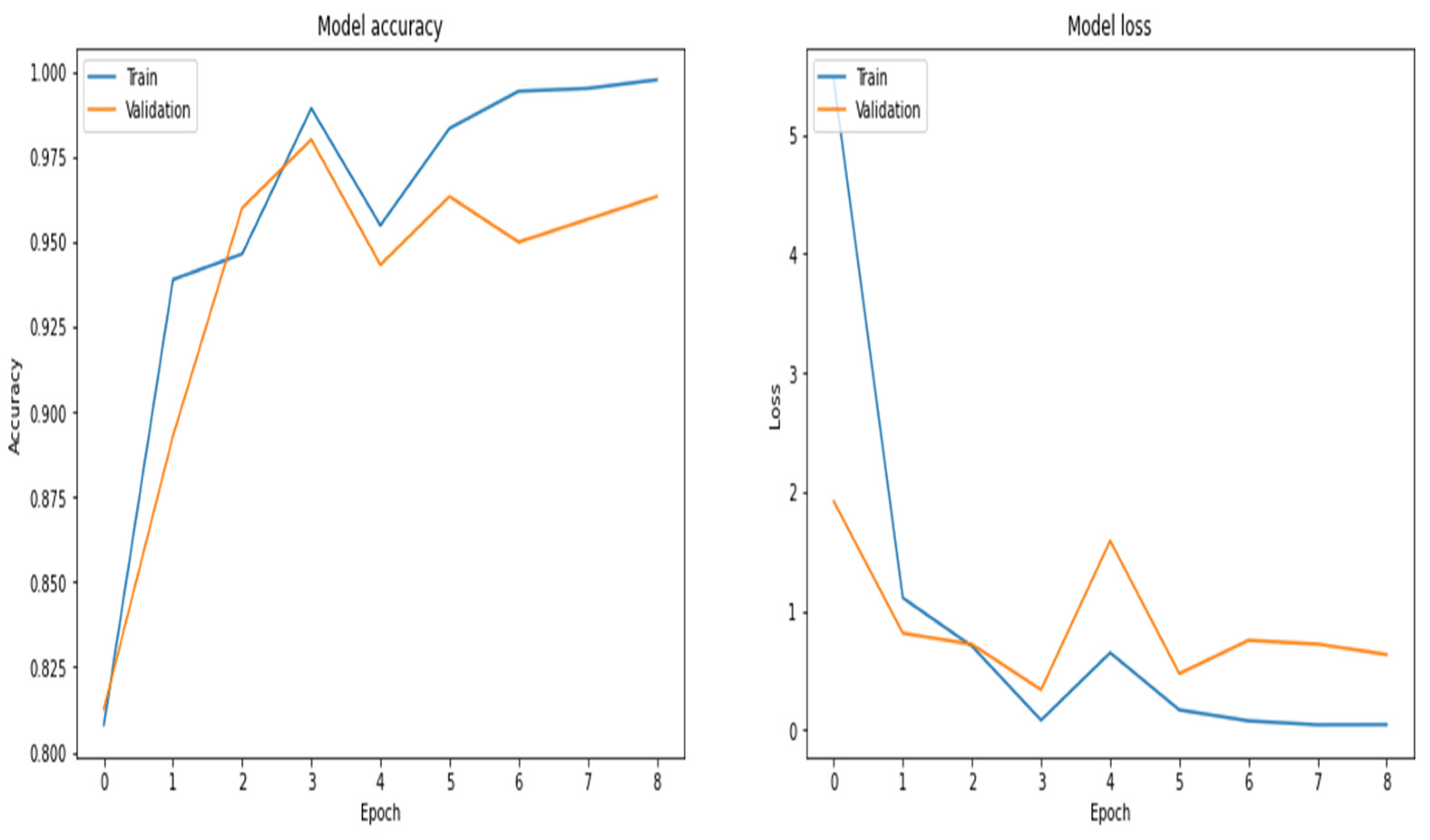
Figure 18.
Accuracy and loss curves by using RNN.
Figure 18.
Accuracy and loss curves by using RNN.
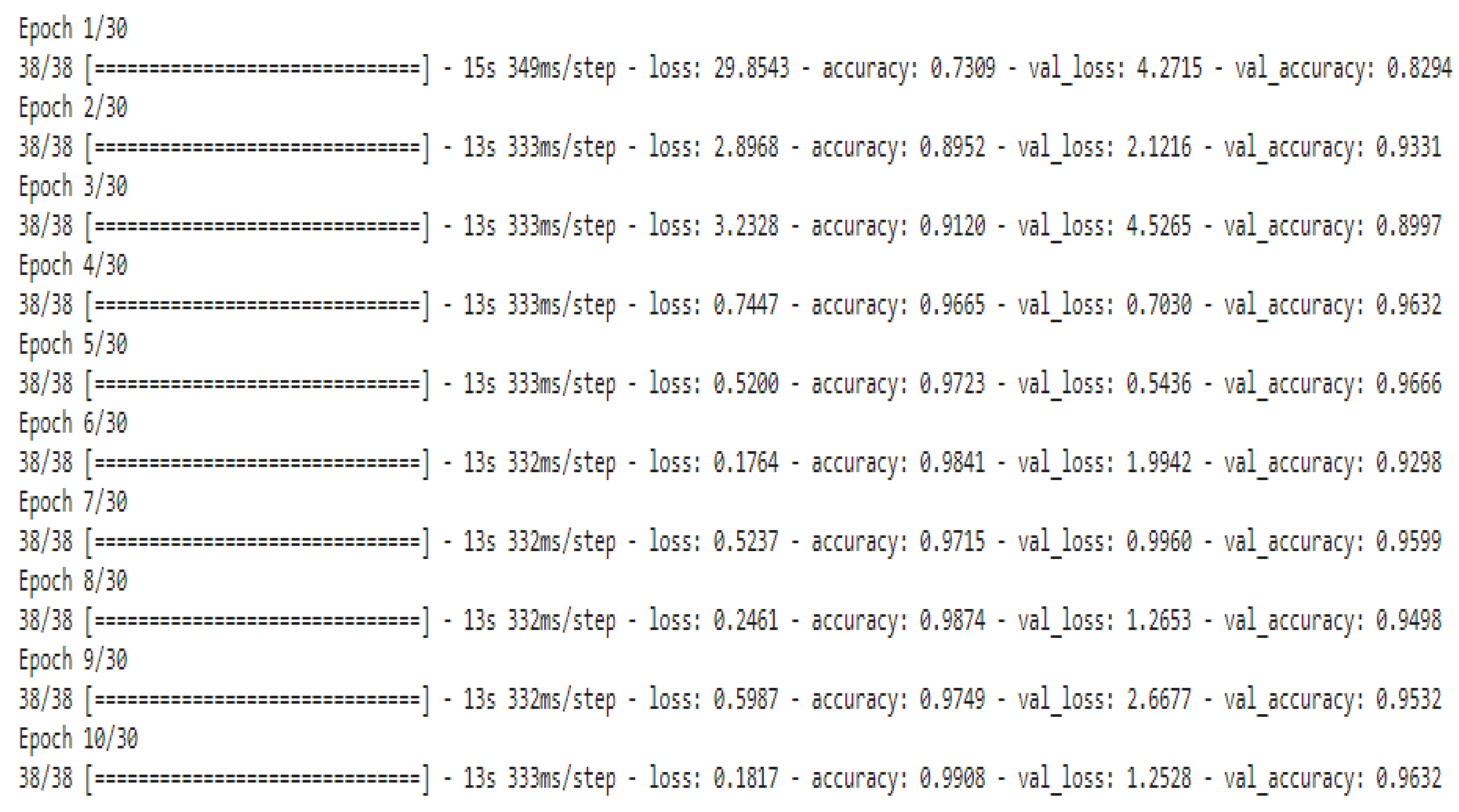
Figure 19.
Fitting results of the LSTM architecture.
Figure 19.
Fitting results of the LSTM architecture.
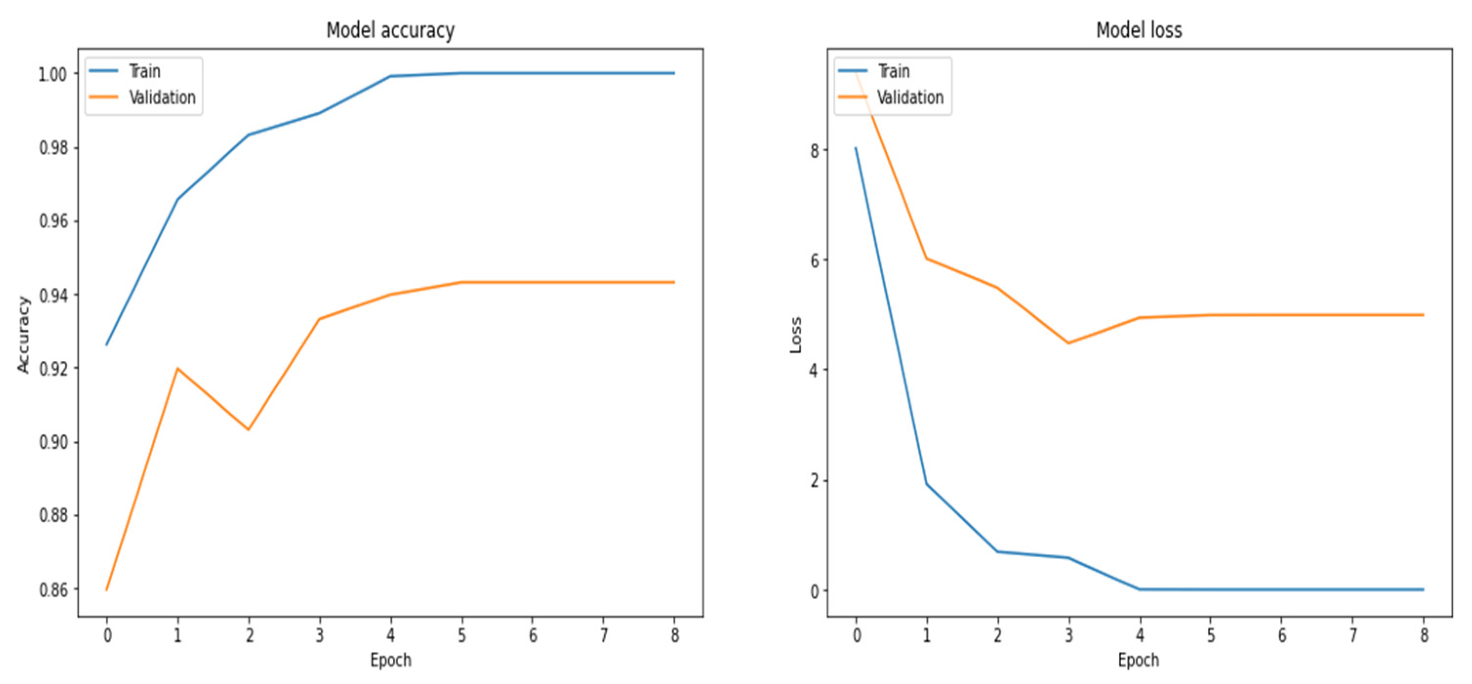
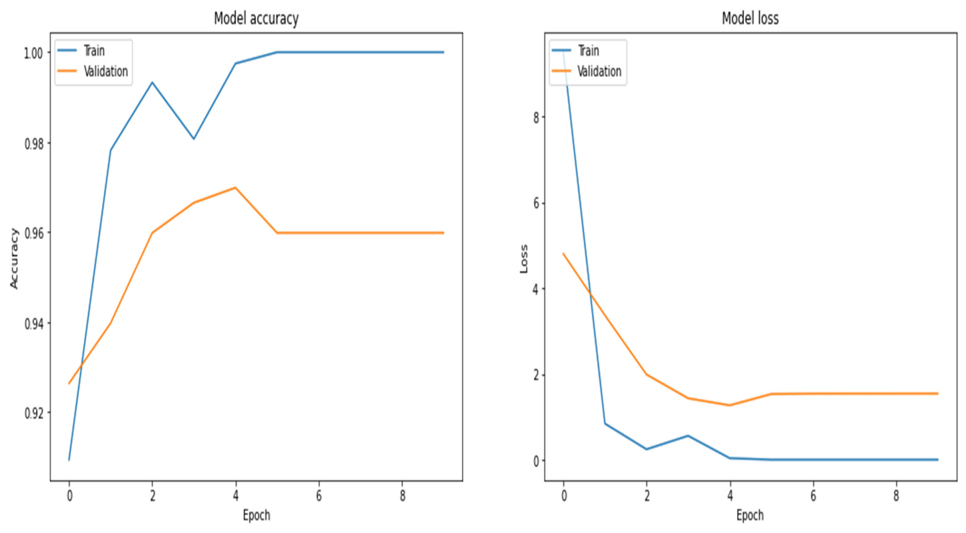
Figure 20.
Accuracy and loss curves using the LSTM model.
Figure 20.
Accuracy and loss curves using the LSTM model.
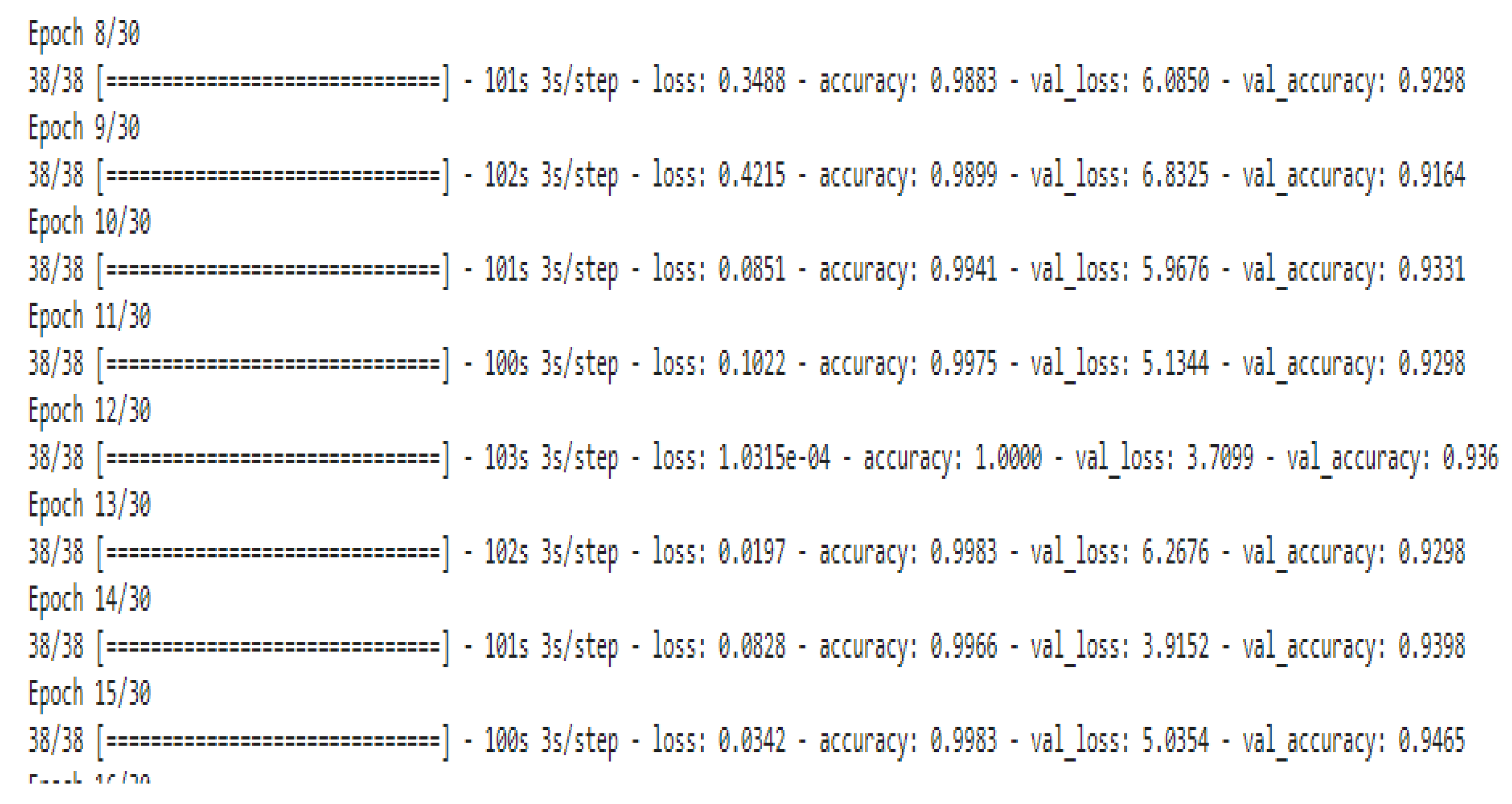
Figure 21.
Fitting results by using the GRU architecture.
Figure 21.
Fitting results by using the GRU architecture.
Figure 22.
Accuracy and loss curves by using the GRU model.
Figure 22.
Accuracy and loss curves by using the GRU model.
Table 1.
List of nomenclature used in this paper.
Table 1.
List of nomenclature used in this paper.
| Nomenclature | Referred to |
|---|
| EEG | Electroencephalogram |
| BCI | Brain–Computer Interface |
| CNN | Convolutional Neural Network |
| RNN | Recurrent Neural Network |
| LSTM | Long Short-term Memory Network |
| GRU | Gated Recurrent Unit |
| DL | Deep Learning |
| ML | Machine Learning |
| FFNN | Feed Forward Neural Network |
| NLP | Natural Language Processing |
| TP | True Positive |
| TN | True Negative |
| FP | False Positive |
| FN | False Negative |
Table 2.
Keras implementation of the RNN model.
Table 2.
Keras implementation of the RNN model.
| Model: “model” | | |
| Layer (type) | Output Shape | Param # |
| input_1 (InputLayer) | (None, 2548) | 0 |
| tf.expand dims (TFOpLambda) | (None, 2548, 1) | 0 |
| simple rnn (SimpleRNN) | (None, 2548, 128) | 16,640 |
| flatten (Flatten) | (None, 326144) | 0 |
| dense (Dense) | (None, 3) | 978,435 |
| Total params: 995,075 | | |
| Trainable param: 995,075 | | |
| Non-trainable params: 0 | | |
Table 3.
Keras implementation of the LSTM model.
Table 3.
Keras implementation of the LSTM model.
| Model: “model_1” | | |
| Layer (type) | Output Shape | Param # |
| input_2 (InputLayer) | (None, 2548) | 0 |
| tf.expand_dims_1 (TFOpLambda) | (None, 2548, 1) | 0 |
| lstm_1 (LSTM) | (None, 2548, 128) | 66,560 |
| flatten 1 (Flatten) | (None, 326144) | 0 |
| dense_1 (Dense) | (None, 3) | 978,435 |
| Total params: 1,044,995 | | |
| Trainable param: 1,044,995 | | |
| Non-trainable params: 0 | | |
Table 4.
Keras implementation of the GRU model.
Table 4.
Keras implementation of the GRU model.
| Model: “model_3” | | |
| Layer (type) | Output Shape | Param # |
| input_4 (InputLayer) | (None, 2548) | 0 |
| tf.expand_dims_3 (TFOpLambda) | (None, 2548, 1) | 0 |
| gru_1 (GRU) | (None, 2548, 128) | 50,304 |
| flatten 3 (Flatten) | (None, 326144) | 0 |
| dense_3 (Dense) | (None, 3) | 978,435 |
| Total params: 1,028,739 | | |
| Trainable param: 1,028,739 | | |
| Non-trainable params: 0 | | |
Table 5.
Confusion matrix by using RNN model.
Table 5.
Confusion matrix by using RNN model.
| | Negative | Neutral | Positive |
|---|
| Negative | 181 | 1 | 19 |
| Neutral | 0 | 222 | 9 |
| Positive | 9 | 2 | 197 |
Table 6.
Performance measures by using the RNN model.
Table 6.
Performance measures by using the RNN model.
| | TP | TN | FP | FN | Sensitivity/Recall | Specificity | Precision | F1 Score | Accuracy |
|---|
| Negative | 181 | 430 | 9 | 20 | 0.90 | 0.97 | 0.95 | 0.92 | 0.95 |
| Neutral | 222 | 406 | 3 | 9 | 0.96 | 0.97 | 0.98 | 0.96 | 0.98 |
| Positive | 197 | 404 | 28 | 11 | 0.94 | 0.97 | 0.87 | 0.89 | 0.93 |
| Average results | 0.93 | 0.97 | 0.93 | 0.92 | 0.95 |
Table 7.
Confusion matrix of LSTM model.
Table 7.
Confusion matrix of LSTM model.
| | Negative | Neutral | Positive |
|---|
| Negative | 194 | 0 | 7 |
| Neutral | 0 | 227 | 4 |
| Positive | 8 | 2 | 198 |
Table 8.
Performance measures of the LSTM model.
Table 8.
Performance measures of the LSTM model.
| | TP | TN | FP | FN | Sensitivity/Recall | Specificity | Precision | F1 Score | Accuracy |
|---|
| Negative | 194 | 431 | 8 | 7 | 0.96 | 0.98 | 0.96 | 0.95 | 0.97 |
| Neutral | 227 | 407 | 2 | 4 | 0.98 | 0.99 | 0.99 | 0.98 | 0.99 |
| Positive | 198 | 421 | 11 | 10 | 0.95 | 0.97 | 0.94 | 0.94 | 0.96 |
| Average results | 0.96 | 0.98 | 0.96 | 0.95 | 0.97 |
Table 9.
Confusion matrix of the GRU model.
Table 9.
Confusion matrix of the GRU model.
| | Negative | Neutral | Positive |
|---|
| Negative | 194 | 0 | 7 |
| Neutral | 0 | 228 | 3 |
| Positive | 12 | 4 | 192 |
Table 10.
Performance measures of the GRU model.
Table 10.
Performance measures of the GRU model.
| | TP | TN | FP | FN | Sensitivity/Recall | Specificity | Precision | F1 Score | Accuracy |
|---|
| Negative | 194 | 427 | 12 | 7 | 0.96 | 0.97 | 0.94 | 0.94 | 0.97 |
| Neutral | 228 | 405 | 4 | 3 | 0.98 | 0.99 | 0.98 | 0.98 | 0.98 |
| Positive | 192 | 422 | 10 | 16 | 0.92 | 0.97 | 0.95 | 0.93 | 0.95 |
| Average results | 0.95 | 0.97 | 0.95 | 0.95 | 0.96 |
Table 11.
Performance metrics of RNN, LSTM and GRU models.
Table 11.
Performance metrics of RNN, LSTM and GRU models.
| S. No. | Network | Sensitivity | Specificity | Precision | F1 Score | Accuracy |
|---|
| 1 | RNN | 0.93 | 0.97 | 0.93 | 0.92 | 0.95 |
| 2 | LSTM | 0.96 | 0.98 | 0.96 | 0.95 | 0.97 |
| 3 | GRU | 0.95 | 0.97 | 0.95 | 0.95 | 0.96 |
Table 12.
Comparative analysis with other existing works for EEG emotion detection.
Table 12.
Comparative analysis with other existing works for EEG emotion detection.
| Method/Author | Average Accuracy Rate (%) |
|---|
| DNN+ Sparse Auto encoder/[23] | 96 |
| DCNN/[24] | 85 |
| Multi column CNN/[25] | 90 |
| 3D CNN/[26] | 88 |


