Abstract
The inspection of gray matter (GM) tissue of the human spinal cord is a valuable tool for the diagnosis of a wide range of neurological disorders. Thus, the detection and segmentation of GM regions in magnetic resonance images (MRIs) is an important task when studying the spinal cord and its related medical conditions. This work proposes a new method for the segmentation of GM tissue in spinal cord MRIs based on deep convolutional neural network (CNN) techniques. Our proposed method, called MobileUNetV3, has a UNet-like architecture, with the MobileNetV3 model being used as a pre-trained encoder. MobileNetV3 is light-weight and yields high accuracy compared with many other CNN architectures of similar size. It is composed of a series of blocks, which produce feature maps optimized using residual connections and squeeze-and-excitation modules. We carefully added a set of upsampling layers and skip connections to MobileNetV3 in order to build an effective UNet-like model for image segmentation. To illustrate the capabilities of the proposed method, we tested it on the spinal cord gray matter segmentation challenge dataset and compared it to a number of recent state-of-the-art methods. We obtained results that outperformed seven methods with respect to five evaluation metrics comprising the dice similarity coefficient (0.87), Jaccard index (0.78), sensitivity (87.20%), specificity (99.90%), and precision (87.96%). Based on these highly competitive results, MobileUNetV3 is an effective deep-learning model for the segmentation of GM MRIs in the spinal cord.
1. Introduction
The presented research work deals with spinal cord (SC) gray matter (GM) segmentation, which plays an important role in human diagnoses and assessments of the SC. The spinal cord is a column of nerve tissue that runs from the skull base down the back’s center. Spinal cord nerves carry messages between the brain and the rest of the body [1]. Identifying the part of the small butterfly or H-shaped structure of the spinal cord is broadly known as gray matter segmentation. GM is challenging to image and delineate from its surrounding white matter (WM) due to its small and intricate shape [2]. Magnetic Resonance Imaging (MRI) of the spinal cord gray matter at the cervical and lumbar regions may be particularly informative in lower motor neuron disorders [3]. Standardized datasets in this area continue to be a significant problem due to the variability in equipment from different vendors, acquisition protocols, parameters used, and generated image contrasts. Furthermore, data availability is limited due to concerns around ethics and regulations on patient data privacy [4].
The spinal cord is thus an indispensable, yet sensitive part of the central nervous system. The ability to differentiate and identify the structure of the spinal cord, such as gray matter vs. white matter, is paramount for the evaluation of therapeutic interventions and the prognosis of relevant neurological medical conditions. The availability of new magnetic resonance imaging (MRI) sequences has enabled the clinical study of the spinal cord’s internal structure in vivo. Nonetheless, the presence of artifacts, image distortions, and the low contrast-to-noise ratio have substantially limited the use of tissue segmentation techniques previously developed for the central nervous system. Furthermore, because of the inter-subject variability displayed in cervical magnetic resonance images (MRIs), typical deformable volumetric registration techniques have performed poorly [5], thus reducing the adoption of multi-atlas segmentation methods. Until recently, this has prevented the development of automated segmentation algorithms for the spinal cord’s internal structure. An integral part of digital image processing when using spinal cord magnetic resonance imaging (MRI) is the ability to segment gray and white matter accurately and reliably, in order to perform tissue specific analysis. Image segmentation methods can be divided into two broad categories: semi-automated and fully automated. There are various semi- or fully automated segmentation techniques for cervical cord cross-sectional area measurements that give a good performance that is near or equal to manual segmentation, which is the gold standard in this case. However, in gray matter segmentation, the challenge is in dealing with a cross-sectional area whose size and shape are small. Ongoing research is being undertaken by a number of teams around the world to find a solution to this problem [3,6,7,8,9,10,11].
The work in [3] describes a framework for the segmentation of cervical spinal cord MRI using a slice-based approach. In particular, a technique is presented for pre-alignment of the slice-based atlases into a space comprised of consistent groups. In addition to modeling of spinal cord variability, the method generated segmentations while using atlas information that is suitably geodesical. Results obtained from a cross-validation experiment using 67 MR volumes of the cervical spinal cord showed high accuracy at the sub-millimetric level [3]. Recently, a spinal cord gray matter (SCGM) segmentation challenge was organized to evaluate the performance of several methods using the same dataset obtained from multiple research centers and vendors, while generated using different three-dimensional gradient-echo sequences [6]. The goals of this challenge were to present the advancements in the field and to determine new opportunities for future work. In this competition, a number of distinct spinal cord gray matter segmentation techniques were compared to the results obtained by manual segmentation. Each of these techniques was independently developed by a different research team throughout the world. Overall, the included methods yielded good results for gray matter butterfly detection with some variations in the performance of a few metrics. For the many researchers working in this area throughout the world, a beneficial outcome of this challenge competition has been the public availability of a standardized medical dataset [7].
Another medical condition of pertinent importance is the irreversible clinical disability in multiple sclerosis (MS) patients that can be caused by axonal loss. The assessment of in-vivo axonal loss may be indirectly performed by estimating the reduction over time in the cervical cross-sectional area (CSA) of the spinal cord. Such a measure is crucial in indicating the level of spinal cord atrophy. Applying segmentation of images obtained via MRI may yield an accurate estimation of said measure. In [7], the authors present an automated spinal cord segmentation technique that includes the Optimized PatchMatch Label (OPAL) fusion algorithm for determining the location and providing an approximate segmentation of the spinal cord, as well as the Similarity and Truth Estimation for Propagated Segmentations (STEPS) for the simultaneous segmentation of white and gray matter. In analyzing MRI data of a case-control study, the described method resulted in obtaining CSA measurements that have an identical accuracy to the inter-rater variability, with a high value of the dice similarity coefficient (DSC) at the C2/C3 level [8]. In addition, a Gray Matter Segmentation Based on Maximum Entropy (GSBME) algorithm, comprising three stages, using semi-automatic supervised segmentation is further elaborated on in [7]. The first stage involves pre-processing of the image undertaken for the detection of the spinal cord followed by signal normalization. The second stage deals with thresholding of the entropies of gray and white matter signal intensity. The third step handles the detection of outliers. The segmented hyperintensities are discarded based on their morphological features, such as perimeter and eccentricity, using a data description toolbox, known as DDTools [7].
A publicly available implementation of the Morphological Geodesic Active Contour (MGAC) algorithm coupled with the software package Jim from Xinapse Systems, as the tool for spinal cord segmentation, were used to estimate the initial boundary of the spinal cord in [8]. Two-dimensional phase-sensitive inversion recovery (PSIR) images of the C2/C3 level with two different resolutions, two-dimensional T2 weighted images of the C2/C3 level, and a three-dimensional PSIR image were employed to show the workings of the MGAC algorithm. To evaluate the accuracy of the segmentations, visual assessment along with two measures—the Hausdorff distance and the dice similarity coefficient—were utilized [8].
In the work presented in [9], the Spinal Cord Toolbox (SCT) method used for segmentation, rooted in an atlas-based approach, was developed with information at the vertebral level and the normalization of linear intensity in order to handle data from multiple sites. After building a dictionary of images using WM/GM segmentations by experts, the selected image is pre-processed, normalized, and treated using Principal Component Analysis (PCA). Segmentation is applied using label fusing on the selected dictionary images. SCT is made available as an open-source software for free [9]. The work in [6] also proposes a Variational Bayes Expectation-Maximization (VBEM) algorithm. This is a probabilistic method used for segmentation to learn tissue intensity distributions in MRI scans in a semi-supervised fashion. The image intensities are modeled as random variables taken from a Gaussian mixture distribution, including nonlinearly warped tissue priors. The parameters are estimated using the Expectation-Maximization (EM) method and the algorithm can be employed in an unsupervised manner, or by adopting training data with manually generated labels [6].
DEEPSEG is a development of the deep 3D convolutional encoder network enhanced with shortcut connections [10]. The employed CNN possesses a contracting path to aggregate information. It also has an expanding path to upsample the feature maps to yield a dense output used for prediction. Instead of using upsampling layers as in UNet, they utilize an unpooling and deconvolution strategy. This architecture has eleven layers, and the network is pre-trained thanks to three convolutional restricted Boltzmann Machines. In order to achieve balance between specificity and sensitivity, a special loss function is utilized incorporating a weighted sum of two terms that express the mean square differences of the gray matter and non-GM voxels in the image. Two different models were trained independently for GM segmentation and for full spinal cord segmentation [10].
The project known as Joint Collaboration for Spinal Cord gray matter Segmentation (JCSCS) involves the combination of two existing label fusion segmentation methods [1]. This approach is based on multi-atlas segmentation propagation of 2D sliced images using registration and segmentation. Here, the OPAL method is used to detect and localize the spinal cord with the aid of an external dataset whose images of spinal cord volumes are manually segmented. Then, the STEPS methodology is applied to segment the gray matter using a segmentation propagation step followed by consensus segmentation. The latter step is realized based on locally normalized cross-correlation applied to deformed templates before they are fused [1]. Further, work using Atrous Spatial Pyramid Pooling (ASPP) employs dilated convolutions [11]. In this segmentation architecture, the authors dealt with imbalanced data by using a different loss function, called the Dice Loss, which proved to be insensitive to such unbalancing. Other modifications employed to improve the performance of GM segmentation include the removal of decimation operations from the network and parameter reduction. This allowed for the trading of depth to improve the network’s equivariance. In addition, by using dilated convolutions, it was convenient to substantially enlarge the effective receptive field without grossly increasing the number of parameters, thereby preserving the quality of the input resolution in the entire network. Data augmentation strategies in the form of adding noise, elastic deformation, scaling, shifting, and rotation were also applied to enrich the dataset and achieve good results in a binarized detection of GM and non-GM [11].
It follows that image segmentation is a key part in many image processing and computer vision systems. It is used in a wide range of applications that include, among others, the analysis of medical images, video surveillance, augmented reality, as well as autonomous vehicles [12]. Over the past few years, deep learning (DL) has attracted a lot of attention from the research community in the medical domain to solve image segmentation problems due to its impressive performance in other computer vision fields [3]. The use of DL models in image segmentation has ushered a new era, where performance improvements in accuracy rates are expected to outpace those obtained from earlier image segmentation algorithms such as region growing, watersheds, or active contours to name a few [13]. It is safe to say that the use of DL models in image segmentation tasks has brought about a paradigm shift in this area [14]. In this regard, DL-based semantic segmentation has witnessed an increasing level of interest over the last few years. In particular, UNet, which is one of the deep-learning networks with an encoder-decoder architecture, is widely used in the segmentation of medical images [12]. Moreover, the UNet architecture is better designed, when compared with other algorithms of spinal cord image segmentation, as it learns with fewer training images and produces more accurate segmentation results [5].
In this article, we propose a deep learning UNet-like architecture for the segmentation of gray matter regions in MRIs of the spinal cord based on the pre-trained MobileNetV3 model (large version) [15]. The proposed method is beneficial for objects that appear at varying scales. In addition to accuracy improvements, the proposed model, having been combined with the lightweight MobileNetV3, may reduce the network parameters to improve the computation efficiency and make it less prone to overfitting when handling small datasets. To the best of our knowledge, there are no similar methods in the literature that combines MobileNetV3 with UNet to yield a deep-learning model that is employed in image segmentation. Its effectiveness is demonstrated on the SCGM segmentation challenge dataset. The results of the segmentation performance are highly competitive when compared with recent state-of-the-art models. Our main contributions in this work can be summarized as follows:
- A solution for the segmentation of GM tissue in spinal cord MRIs is presented, based on deep convolutional neural network (CNN) techniques.
- A deep UNet-like architecture for image segmentation, called MobileUNetV3, using MobileNetV3 as a backbone is described.
MobileNetV3 is based on bneck blocks that produce feature maps. These blocks are optimized using residual connections and squeeze-excitation (SE) modules. This has motivated us to adopt it as a base backbone model for a UNet-like architecture. As a result, we anticipate that the combined model would perform well for the planned segmentation task.
- The proposed model was validated with different optimizers and batch sizes for a high number of epochs to enhance its accuracy. It was then evaluated with various performance parameters, such as the dice similarity coefficient, Jaccard index, sensitivity, specificity, and precision. Finally, its performance was compared to seven state-of-the-art machine learning models and found to yield excellent results.
2. Materials and Methods
The proposed model combines the UNet architecture with the MobileNetV3 model for spinal cord gray matter segmentation. We begin this section by elaborating on the employed dataset. Then, we briefly review the UNet architecture for image segmentation. We follow this by presenting the MobileNetV3 model and its main properties. We explain how we combined them together to build our unique segmentation model, called MobileUNetV3, and highlight its major differences with UNet.
2.1. Dataset Description and Pre-Processing
The used dataset was first presented during the Spinal Cord Gray Matter Segmentation (SCGMS) Challenge [7]. The dataset was a collaboration between four internationally recognized spinal cord imaging research groups. These groups were from: (1) University College London, (2) Polytechnique Montreal, (3) University of Zurich, and (4) Vanderbilt University. The dataset consists of 80 healthy subjects, with 20 subjects contributed from each center. The demographics range from a mean age of 28.3 up to 44.3 years old. Three different MRI systems were used (Philips Achieva, Philips, Inc., Florida, USA; Siemens Trio andSiemens Skyra, Siemens, Inc., Erlangen, Germany) with different acquisition parameters based on a multi-echo gradient echo sequence. The voxel size ranges from 0.25 mm × 0.25 mm × 2.5 mm up to 0.5 mm × 0.5 mm × 5.0 mm.
The MR image captured from each subject is a 3D volume with size R × C × S, which stands for rows, columns, and slices, respectively. Figure 1 shows the MRI volume captured for subject 1 of site 1, which is composed of three slices. These slices represent views at certain cut locations from the spinal cord, as indicated by the colored horizontal lines on the left part of the figure.
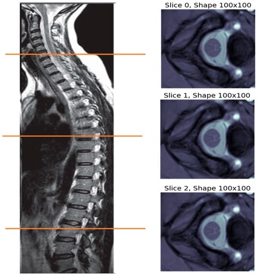
Figure 1.
MRI volume for subject 1 of site 1, which is made up of three MRI slices captured at certain locations in the subject’s spine, as indicated by the colored horizontal lines.
The dataset is split between training (40 images) and testing (40 images). Subjects 1 to 10 from all four sites are used for training while the remaining subjects from 11 to 20 are used for testing. Furthermore, one segmentation mask was produced by an expert for each image. The image sizes as well as the number of slices taken from each subjects vary. Table 1, Table 2 and Table 3 show the range and distribution of the volume shapes in the dataset. The shapes range from (100 × 100 × 3) to (655 × 776 × 28) voxels. Subjects 1 to 10, used for training, as well as subjects 11 to 20, used for testing, are all different from one site to another, respectively.

Table 1.
Distribution of MRI slices, used for training, by different subjects and sites.
Table 2.
Distribution of MRI slices, used for testing, by different subjects and sites.
Table 3.
Distribution of volume shapes in the dataset. All 80 images are considered. The first three digits from the bottom represent the first dimension followed by another set of three digits for the second dimension. The two rows before the top one give the value of the third dimension.
Some methods in the literature, such as DEEPSEG in [10], use the whole 3D MRI volume as an input to their segmentation method. However, most other approaches use the slices as separate images. We follow this latter approach because it enables us to exploit the wealth of pre-trained CNN models, which are trained on separate RGB images. In any case, 2D convolutional operations are more computationally efficient compared with 3D ones. Furthermore, it is well known that deep-learning models prefer large image datasets, with thousands or millions of images, for better training. For example, the well-known ImageNet dataset contains more than 14 million images [16,17]. Hence, working on separate slices is more effective because it provides us with a larger dataset. For the dataset at hand, the total number of slices used for training was 551 while 541 slices were used for testing. On the other hand, a dataset with about 1000 images would still be considered modest, and the larger the deep-learning model is, the more it is in need of larger image datasets. Thus, our proposed solution based on a light CNN model, such as MobileUNetV3, is well justified considering the rather modest and limited dataset size of 1092 available SCGM magnetic resonance images [18].
In Figure 2, we present a sample of the MRI slices and its true segmentation mask. We highlight in this figure the so-called white and gray matter regions in the spinal cord. It is important to note here that the MRI slice is not a typical RGB image with pixel values ranging from 0 (darkest) to 255 (brightest). The type of pixel values in the MRI slices are real valued and have a wide magnitude range. The varied green color in the figure is used only for visualization and does not have any medical meaning.
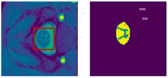
Figure 2.
(left) Image slice of the spinal cord’s white matter (WM) and gray matter (GM). (right) WM and GM true-mask segmentation. The red rectangle shows the area of interest in the spinal cord displaying both gray matter and white matter.
The variability in the sizes of the MRI slices also creates a challenge for deep CNN models, because they require all input images to have a fixed size. Thus, fixing the size of the slices in the dataset is an important first step. One standard solution employed by many methods in the literature is to simply resize the images to a fixed size. However, we believe that this will introduce unnecessary aspect ratio distortions. This is especially true upon inspection of sample slices in Figure 3, Figure 4, Figure 5 and Figure 6 below, where we observed that the targeted GM region of interest was always at the center of the slice. Thus, we opted for another solution, where we simply crop a window of size 224 × 224 at the center of each slice. We selected the size of 224 × 224 because it is a standard size used in machine learning. Figure 3, Figure 4, Figure 5 and Figure 6 display slices of SCGM MRIs from subject 10 of each site, followed by the resulting cropped images. For site 1, the slice sizes are 100 × 100, which is less than the target size. Thus, instead of cropping the slices, they are padded with zeros.
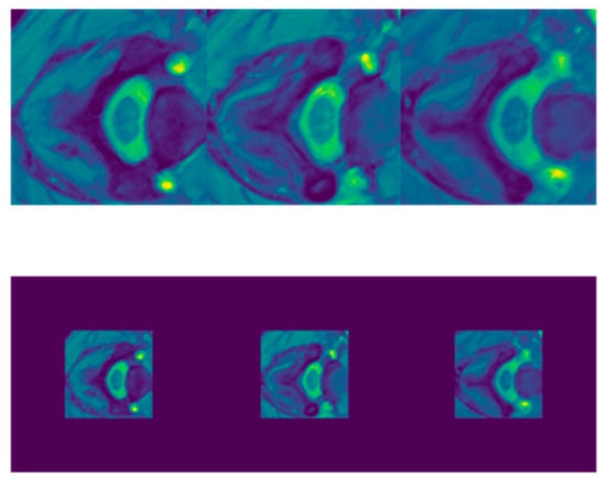
Figure 3.
Slices of SCGM MRIs of subject 10 from site 1. Original image size is 100 × 100. Top row displays original images while the bottom one shows the corresponding padded slices.
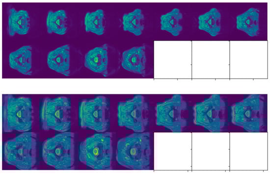
Figure 4.
Slices of SCGM MRIs of subject 10 from site 2. Original image size is 320 × 320. A white square indicates the absence of an MRI slice. Original slices are displayed in the top row while cropped ones are exhibited in the bottom one.
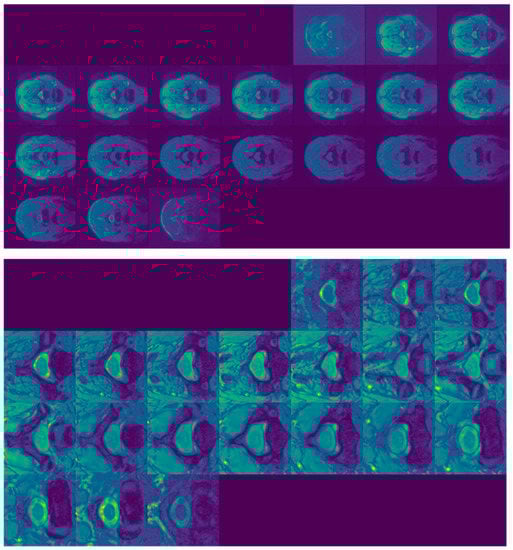
Figure 5.
Slices of SCGM MRIs of subject 10 from site 3. Original image size is 654 × 774. A dark square indicates that the slice does not contain any gray or white matter. Original slices are displayed in the top row while cropped ones are exhibited in the bottom one.
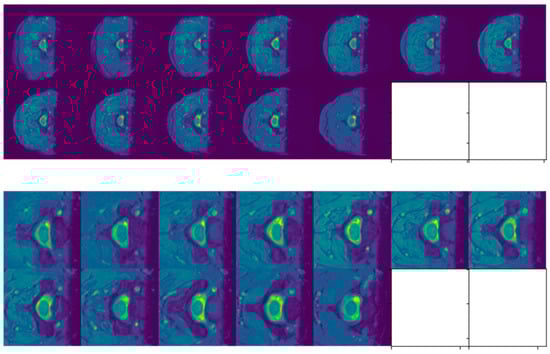
Figure 6.
Slices of SCGM MRIs of subject 10 from site 4. Original image size is 512 × 512. Original slices are displayed in the top row while cropped ones are exhibited in the bottom one.
As far as we know, no previous work that we have reviewed has made a similar detailed presentation about the dataset. This includes the original research paper [7], which introduced the SCGM Challenge. We have emphasized in our coverage of the SCGM Challenge dataset the pre-processing steps that we had to go through to prepare the data for training and eventual testing of the model. The SCGM Challenge dataset used and analyzed during the current study is publicly available on the SCGM Challenge repository at http://rebrand.ly/scgmchallenge (accessed on 24 January 2021).
2.2. UNet Model
UNet is a deep-learning neural network model that was introduced for biomedical image segmentation in [12]. An illustration of UNet architecture is shown in Figure 7, where we can see that it contains two segments. The left segment is called the contraction path (also known as the encoder) and is used to extract multi-scale features from the image. The contraction path is just a sequence of convolutional and max-pooling layers. The right segment is the symmetric expanding path (also known as the decoder) and is used to enable precise localization of the image regions using transposed convolutions. Thus, UNet is an end-to-end Fully Convolutional Network (FCN), i.e., it only contains convolutional layers and does not contain any fully connected layers.
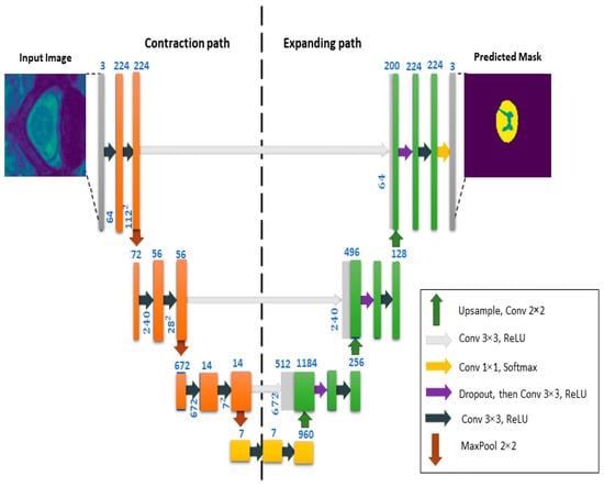
Figure 7.
General overview of the architecture of the UNet model.
2.3. MobileNetV3
MobileNet is a family of Convolutional Neural Networks (CNN) for image classification proposed by a team researchers at Google, Inc. [19]. Through its different versions, MobileNet introduced many novel ideas aimed at reducing the number of parameters to make it more efficient for mobile devices, yet at the same time achieving high classification accuracy. These novel ideas include the depth-wise convolution, Squeeze-Excitation (SE) modules, Inverted Residual Block (IRB), and a new activation function, called h-swish. According to [20], MobileNet yields high performance in terms of accuracy as a function of MADDS (multiply-add operations), when compared with many other CNN architectures of similar size. In particular, MobileNetV3 has the highest top-1 accuracy amongst the different models considered by the authors in [20]. This is the main reason that has motivated us to investigate the MobileNetV3 model for this segmentation task.
MobileNet is composed of several blocks called bneck blocks. Figure 8a shows the overall MobileNet architecture, while Figure 8b shows the details inside a bneck block. MobileNetV1 replaced regular convolutional operations by the depth-wise convolutional operations in every block to reduce the number of parameters. A residual connection between the input and output tensors was also added, as illustrated in Figure 8b. Then, in MobileNetV2 [20], the authors added an expansion and compression steps at the beginning and end of each bneck block, as shown in Figure 8. This setup is called Inverted Residual Block (IRB), because the residual connections connect narrow (i.e., low number of channels) input and output tensors, as opposed to the expanded tensors present in the original ResNet CNN model [21].
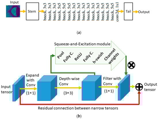
Figure 8.
MobileNet models are composed of a concatenated set of bneck blocks. (a) High level overview. (b) Illustration of a bneck block.
The IRB idea contributed to more reduction in the computation cost of the model. To reduce computations further, the authors also used linear activations after filtering the input and output tensors as opposed to non-linear activation functions (such as ReLU). Finally, the authors added an SE module [22] to the MobileNetV3 model. The SE module and its layers are shown in Figure 8b. However, unlike the other models which add the SE module as a separate block of ResNet [23] or Inception [17,24] CNN models, MobileNetV3 adds it in parallel with the IRB connection as shown in Figure 8b. The addition of the SE module increased the size of the model slightly but improved the accuracy and latency of the model.
The authors also introduced an activation function called h-swish [20] within the SE module. The Swish activation function is defined as follows:
where is the sigmoid function and is a trainable parameter. When , this is known as the sigmoid-weighted linear unit function. However, the computation of this function is computationally expensive, so they introduced the h-swish function, which is given by:
where is a modification of the rectified linear unit, whereby the activation is limited to a maximum size of 6. From the above discussion, we observe that a bneck block produces a feature map that is optimized using residual connections and SE modules. This motivated us to utilize it as a base backbone model for a UNet-like architecture.
2.4. Proposed MobileUNetV3 Architecture
The proposed model combines the UNet architecture with MobileNetV3 for spinal cord GM segmentation in order to exploit its strong feature extraction capabilities, thus the name: MobileUNetV3. The question is how best to combine these two models, which is the main contribution of our research work herein. In Figure 9, we show the architecture of the proposed MobileUNetV3 model, including its different blocks together with the input feature maps. In the encoder part, the selected MobileNetV3 layers are applied with downsampling to reduce the image size. In the decoder part, the upsampling and transposed convolution are applied to generate a segmentation mask for each input image.
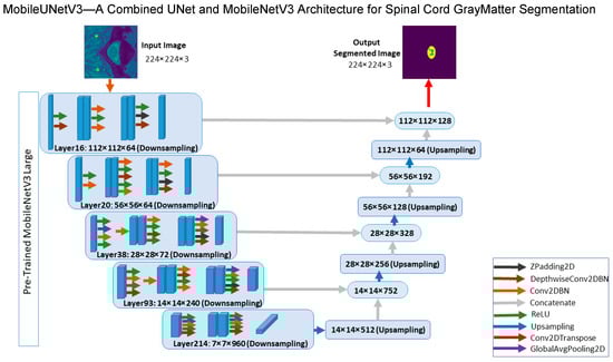
Figure 9.
Architecture of the proposed MobileUNetV3 deep learning model.
The input image of the model is an MRI slice of size 244 × 244. The model takes the input image to MobileNetV3 as a backbone encoder of UNet architecture with the layers (16, 20, 38, 93, 214). We selected these layers because they are activation layers (ReLU) and they have the highest number of convolutional filter bands within their feature map size category (112 × 112, 56 × 56, 28 × 28, and so on). For instance, Layer 16 changes the image size to 112 × 112 with 64 bands. Layer 20 changes the image size to 56 × 56 with 64 bands. Layer 38 changes the image size to 28 × 28 with 78 bands. Layer 93 changes the image size to 14 × 14 with 240 bands. Finally, Layer 214 changes the image size to 7 × 7 with 960 bands. Afterwards, the UNet decoder is used for upsampling and concatenation with the previous output layer and each layer of MobileNetV3. The first upsampling is of Layer 214 with an image size of 14 × 14 with 512 bands, which is then concatenated with output Layer 93. This is clearly depicted in Figure 9 above. Lastly, a deconvolution layer, also called transposed convolution layer, plus a Softmax activation function is used to get the output. The input and output images share the same size. The output of the proposed model is an image mask segmentation of size 244 × 244 with 3 bands, allowing our model to detect three separate classes, for instance GM, WM, and other components in the input image slice (background). We provide a detailed listing of layers and the number of parameters in each decoding layer of our proposed model in Table 4 below. The total number of parameters, both trainable and non-trainable, are also given. Our lightweight model, with 8,045,347 total number of parameters, is easy to train and less prone to overfitting when dealing with small datasets [25].
Table 4.
Details of layers and number of parameters in the proposed model.
The proposed architecture localizes and distinguishes the three channels (GM, WM, Background) by assigning every pixel to the class with the highest output probability. In Figure 10, we illustrate the proposed model, MobileUNetV3, in the form of a concept map.
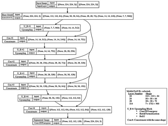
Figure 10.
Illustration of the proposed MobileUNetV3 deep-learning model in the form of a concept map.
To effectively train the MobileUNetV3 model, we optimized a loss function based on cross-entropy (CE) loss, denoted by . The loss is computed over the training set as follows:
where N is the number of training samples and is the number of classes. In addition, is the prediction probability of class k for element x. The term is the true label of sample x and 1() is an indicator function that returns one if the included statement is true, otherwise, it returns zero.
2.5. Differences between MobileUNetV3 and UNet Models
MobileUNetV3 has a UNet-like architecture [12], thus they share a lot of similarities. However, there are some differences. Notably, the contracting path in the UNet model is simpler. It is composed of a series of convolutional layers followed by maxpooling layers, which replace fixed-size patches with the maximum value in that patch resulting in contraction of the feature maps size. The expanding or upsampling part of the UNet model uses deconvolution which reduces the number of feature maps while increasing their dimensions. Feature maps from the contracting part of the network are copied to the expanding part to avoid losing pattern structure in the image.
MobileUNetV3, on the other hand, uses a more sophisticated contracting part based on the MobileNetV3 architecture, which is optimized using an automatic search algorithm to find the best architecture [20]. It contains advanced CNN concepts such as Squeeze-Excitation (SE) modules, Inverted Residual Block (IRB), and a new activation function, called h-swish. Furthermore, the MobileNetV3 is pre-trained on a huge image dataset called ImageNet which has more than 14 million samples, while the original UNet model is trained from scratch on the given dataset. These differences make the contracting part of our proposed model an effective tool for extracting highly descriptive feature maps compared to the original UNet model.
In medical imaging applications, the number of images in available datasets is quite limited compared to datasets in other fields, such as ImageNet. This leads to difficulty in training deep models from scratch because that can easily lead to the over-fitting problem. Over-fitting means that the model learns the labeled training samples perfectly, while at the same time not generalizing well to new unseen samples. Our proposed model avoids the problem of over-fitting, by using a pre-trained contracting part. Fine-tuning a pre-trained model is known as transfer learning in the machine learning field and usually produces better results than the training from scratch approach, especially for small datasets.
2.6. Experimental Setup and Evaluation Metrics
In this experimental study, we first took the SCGM challenge dataset and divided each 3D MRI image into slices, then we performed cropping of these slices to get images of sizes equal to 224 × 244 × 3. We also applied the same cropping operations to the corresponding annotated segmentation masks. The actual mask was produced by an expert that segments the gray matter and white matter from a specific image. In order to study the model training behavior, we split the training set into 80% of the images for training and the remaining 20% for validation. In this regard, forty participant images in the training dataset were divided into 551 slices, where we trained the model on 440 of them and validated the model on the remaining 111 slices. Afterwards, we tested the model on the 541 slices of the remaining 10 subjects (subject 11 to 20) of each site. Our experiments were conducted using the open-source library TensorFlow for machine learning. The corresponding Python programs were run using Google’s Colab environment.
To evaluate the proposed method, we followed the trend in the literature and selected useful metrics as in [7]. These metrics include the dice similarity coefficient (DSC), which is a measure of the spatial overlap between two masks. The second metric is the sensitivity (also known as recall, hit rate, or TPR for True Positive Rate). It represents a method’s ability to segment GM as a proportion of all correctly labeled voxels. The third metric is the specificity (also known as selectivity or TNR for True Negative Rate). It measures the ratio of correctly segmented background (non-GM) voxels. The fourth metric is the precision (also known as Positive Predictive Value or PPV), which measures the degree of compromise between true and false positives. Finally, a fifth metric called the Jaccard index (JI) was included. It is a similarity index between two masks and is known to be related to the DSC. These five metrics are defined by the following five equations, where parameters GT and PM refer to ground truth and provided mask, respectively. In addition, a voxel is classified as true positive (TP) if it was a GM voxel in GT mask and it was segmented as GM. A voxel is classified as true negative (TN) if it was a non-GM voxel in GT mask and it was segmented as non-GM. A voxel is classified as false positive (FP) if it was a non-GM voxel in GT mask and it was segmented as GM. Finally, a voxel is classified as false negative (FN) if it was a GM voxel in GT mask and it was segmented as non-GM. We note here that these metrics are computed over the 3D MRI volume and not the individual slices. Then, the overall metric is computed as an average over all subjects in the training or testing set.
3. Results and Discussion
We discuss in this section the results obtained by using the proposed MobileUNetV3 deep-learning model in the segmentation task of SCGM MRIs. We present an experimental analysis of the results that includes the provision of accuracy and loss curves for training and validation, a description of performed visual analysis of segmented test images of SCGM, and an analysis of the obtained segmentation metrics. These metrics are tabulated using the notational format of mean (standard deviation) values, where the corresponding statistics were obtained after averaging over five runs and across all 40 subjects (10 subjects from each of the four sites used for testing).
3.1. Analysis of Results Based on Different Optimizers
We describe herein the segmentation results generated by using the following three optimizers: stochastic gradient descent (SGD), adaptive moment estimation (Adam), and root mean-squared propagation (RMSProp) with a batch size of 8 and up to 400 epochs. We used these optimizers with a varying learning rate, that starts at 0.001 for the first 200 epochs and 0.0001 for the remaining 200 epochs.
In CNN and other neural network-based algorithms, gradient descent is used to minimize the error function during the training process and then updating the internal parameters. In general, an optimization technique is categorized as first-order optimization algorithm and second-order optimization algorithm. For SGD, the modification is made to the amount of the data being used to update the internal parameters. Rather than including the entire training data, SGD uses a subset of training data in a gradual fashion. It calculates one parameter update based on one small subset of the training data. Then, it re-computes the gradients for other subsets and performs the next parameter update. Each subset is chosen randomly, hence the name. Therefore, SGD usually runs faster. The frequent updates in SGD can provide the possibility to discover new and better local minima [26].
RMSProp was developed to resolve the Adagrad problem, just like Adadelta does. It divides the learning rate by using a running average of squared gradients, which is exponentially decaying [27]. On the other hand, the Adam optimizer computes adaptive learning rates for each parameter. Just like Adadelta and RMSProp, Adam stores squared gradients from the bias-corrected past epoch. In addition, Adam also stores the bias-corrected past average gradient. Both of these values estimate the decaying first moment and second moment of the gradients [28]. For more details about optimizers, we refer the reader to [26,27,28].
3.1.1. Accuracy and Loss Results after Model Training and Validation
The purpose of these results is to exhibit epoch-based evolutions of the obtained loss and accuracy values of the model as it learns. The displayed results are obtained using different optimizers with a batch size of 8 and running up to 400 epochs. Figure 11, Figure 12 and Figure 13 display the curves of training and validation accuracy, as well as the curves of training and validation loss for the three optimizers: SGD, Adam, and RMSProp, respectively. A blue color is used for training and orange for validation. We observe that as the number of epochs increases, the accuracy increases while the loss function decreases for all three optimizers. Overall, the model is learning well and is stable even as the number of epochs is increased. From these results, we notice that the two optimizers, Adam and RMSProp, produce higher accuracy results and lower loss values than SGD.
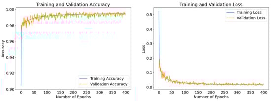
Figure 11.
Accuracy and loss curves generated by SGD optimizer after model training (blue) and validation (orange). A batch size of 8 and 400 epochs are employed.
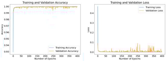
Figure 12.
Accuracy and loss curves generated by Adam optimizer after model training (blue) and validation (orange). A batch size of 8 and 400 epochs are used.
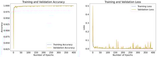
Figure 13.
Accuracy and loss curves generated by RMSProp optimizer after model training (blue) and validation (orange). A batch size of 8 and 400 epochs are utilized.
3.1.2. Visual Analysis of Segmented Images
Figure 14 shows the results of segmentation of a test input image using SGD, Adam, and RMSProp optimizers with a batch size of 8 and using up to 400 epochs. The top row in the figure depicts the input image of SCGM followed by its ground truth mask to the right. The bottom row in the figure shows, from left to right, the three predicted masks of the segmented image for SGD, Adam, and RMSProp optimizers, respectively. From the visual analysis of these predicted masks, we can clearly see that both Adam and RMSProp produce nearly the same result. However, the predicted mask generated by SGD lacks in clarity, where the butterfly profile of the GM in the original image is not fully shown, in addition to the presence of jagged contours in the WM area. Therefore, we can conclude that the SGD optimizer should not be recommended for SCGM segmentation. To select the best performing optimizer among the remaining two, an analysis of their segmentation results in the form of performance metrics will be needed next to differentiate between them.
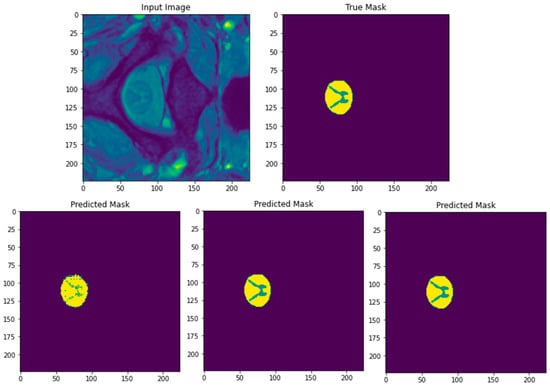
Figure 14.
Original input test image of SCGM and its corresponding ground truth mask (top row). Predicted masks after segmentation with the three used optimizers (bottom row from left to right: SGD, Adam, and RMSProp). A batch size of 8 and 400 epochs are applied.
3.1.3. Analysis Using Performance Metrics
We report the results of segmentation using the five metrics described previously. Although we are mainly interested in the values obtained via only the Adam and RMSProp optimizers in order to compare between them, we provide all three sets of results for the sake of completeness. The comparison between the two optimizers Adam and RMSProp shall allow us to select the optimizer of choice for the rest of this study. Table 5 shows the values of the dice similarity coefficient (DSC), sensitivity, specificity, precision, and Jaccard index (JI) obtained from using the validation dataset by each of the three optimizers: SGD, Adam, and RMSProp. By comparing the values of these five metrics between Adam and RMSProp, we observed that RMSProp provides higher values for DSC, sensitivity, and JI, while Adam yields a slightly higher precision metric. Both optimizers produce similar values in specificity. Therefore, from these results, we can state that the RMSProp optimizer has provided the best results in the segmentation of SCGM. Hence, we will solely be using RMSProp for the remainder of this study.
Table 5.
Obtained values of five segmentation metrics using the three optimizers: SGD, Adam, and RMSProp. For each optimizer, a batch size of 8 samples and 400 epochs are utilized.
3.2. Impact of Different Batch Sizes
In this section, the segmentation results are generated using the RMSProp optimizer on different batch sizes. The batch size is one of the important hyper-parameters in training deep-learning models. Intuitively, training the model on more data should make it learn better. However, there are some practical hardware limitations in terms of the size of random access memory (RAM) available in the employed computing platform. In addition, having a small batch size may be beneficial in training the model, because we will have more update steps, which in turn may improve its learning.
Another motivation is to avoid the well-known “generalization gap” that manifests in the training of deep-neural networks when using large batch sizes [29]. This phenomenon may induce a degradation in the generalization performance of the network and thus, a deterioration of the model’s performance in terms of accuracy, time of convergence, and possibly more, as indicated in [29,30]. One explanation of this situation is the high likelihood of the network, when trained with large batch sizes, converging to sharp minima compared with when trained with small batch sizes [29]. Hence, providing an analysis based on batch size variation is needed to find the corresponding size for which the model learns best, and to mitigate the potential issue related to the model’s generalization performance.
It is important to note that it is perfectly possible that the SGD and Adam optimizers may provide better results on different combinations of batch size and number of epochs. We trained the model for 400 epochs while monitoring the loss and accuracy for the training and validation data. We used the RMSProp optimizer with a varying learning rate, that starts at 0.001 for the first 200 epochs and 0.0001 for the remaining 200 epochs.
3.2.1. Accuracy and Loss Results after Model Training and Validation
The disclosed results are computed using different batch sizes with the RMSProp optimizer running for 400 epochs. Figure 15, Figure 16 and Figure 17 exhibit the curves of training and validation accuracy as well as the curves of training and validation loss for the following three batch sizes: 8, 16, and 32, respectively. A blue color is used for training and orange for validation. We note that larger batch sizes were not possible due to the limited memory capacity exhibited by the employed computing platform. By inspecting these results, we note that as the number of epochs increase, accuracy increases while the loss function decreases for all three considered batch sizes. Additionally, from these results—and because the number of epochs is quite large for our proposed model—it appears that all three batch sizes produce similar results in terms of accuracy and loss values. We expect that the next set of experiments, concerned with the visual analysis of segmented images, will produce more discernable outcomes.
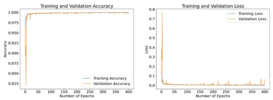
Figure 15.
Accuracy and loss curves generated by RMSProp optimizer after model training (blue) and validation (orange) using a batch size of 8 samples and up to 400 epochs.
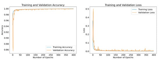
Figure 16.
Accuracy and loss curves generated by RMSProp optimizer after model training (blue) and validation (orange) using a batch size of 16 samples and up to 400 epochs.
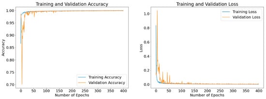
Figure 17.
Accuracy and loss curves generated by RMSProp optimizer after model training (blue) and validation (orange) using a batch size of 32 samples and up to 400 epochs.
3.2.2. Visual Analysis of Segmented Images
Figure 18 displays the results of segmentation of the input image achieved by our model using the RMSProp optimizer, running for 400 epochs with batch sizes of 8, 16, and 32. The top row in the figure depicts the input image of SCGM followed by its ground truth mask to the right. The bottom row in the figure shows, from right to left, the three predicted masks of the segmented image for batch sizes of 8, 16, and 32, respectively. From the visual analysis of these predicted masks, we can clearly see that both batch sizes of 8 and 16 generate nearly the same result, whereas the predicted mask generated by using a batch of 32 samples (leftmost image in bottom row) lacks in clarity where the butterfly profile of the GM in the original image is not as completely shown, in addition to the presence of jagged contours at the border with the WM area. Therefore, we can conclude that using a batch size of 32 samples should not be recommended for SCGM segmentation. To select the best performing batch size among the remaining two, an analysis of their segmentation results in the form of performance metrics will be needed next to make a distinction between them.
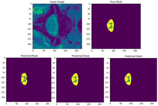
Figure 18.
Original input image of SCGM and its corresponding ground truth mask (top row). Predicted masks after segmentation with the three employed batch sizes (bottom row from right to left: batch size = 8, 16, and 32, respectively). The RMSProp optimizer along with 400 epochs are adopted in these experiments.
3.2.3. Analysis Using Performance Metrics
Although the batch size of 32 has been omitted from further consideration in our study, we present herein all three sets of results for the sake of completeness. The comparison between the two remaining batch sizes of 8 and 16 shall help us select the one to be included for the rest of this study. Table 6 shows the values of the dice similarity coefficient (DSC), sensitivity, specificity, precision, and Jaccard index (JI) obtained by each of the three batch sizes: 8, 16, and 32. By comparing the values of these five metrics delivered by utilizing just the two considered batch sizes, we observed that employing a batch size of 8 samples yields higher values for DSC, sensitivity, and JI, whereas a batch size of 16 samples provides a higher precision metric after applying MobileUNetV3. Both of these batch sizes produce similar values in specificity. Therefore, from these results, we can state that the batch size of 8 has provided the best outcomes in the segmentation of SCGM images. It is nonetheless sensible to mention that it is quite possible that batch sizes 16 and 32 could provide better results on different combinations of epoch values.
Table 6.
Obtained values of five segmentation metrics using three batch sizes of 8, 16, and 32 with the RMSProp optimizer after 400 epochs of running MobileUNetV3.
3.3. Visual Analysis of Segmented Images from Different Sites
We further show in Figure 19 the results of SCGM segmentation of four different MRI slices, each taken from a different site after testing the learning achieved by our proposed deep-learning model with optimizer RMSProp, with a batch size of 8 and up to 400 epochs. The figure exhibits the predicted and true mask of each segmented MRI slice. We observed that, regardless of the location and size of the GM in these input images, our model achieves good segmentation outcomes. These results enhance the usefulness of the model and demonstrate its robustness. Consequently, we shall select this batch size, along with the RMSProp optimizer, when we next compare our model with state-of-the-art methods.
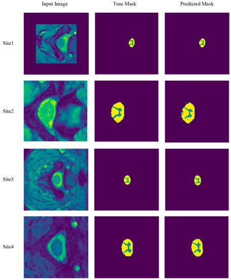
Figure 19.
Segmentation results of four MRI slices from the four previously mentioned sites. The following slices are selected from sites 1, 2, 3, and 4, respectively: Slice 1 from subject 15, slice 13 from subject 11, slice 6 from subject 15, and slice 1 from subject 11. The RMSProp optimizer, a batch size of 8, and 400 epochs are employed with MobileUNetV3 in this set of experiments.
3.4. Comparison with State-of-the-Art Methods
A comparison of our proposed model, MobileUNetV3, with other current state-of-the-art methods using MRIs from the SCGM Challenge dataset was undertaken based on the five metrics: DSC, JI, sensitivity, specificity, and precision. Table 7 provides a list of the seven methods included in this comparison, as well as the achieved scores in each of the five metrics, as obtained from the literature in [11]. We have briefly reviewed each one these seven methods in Section 1. The tabulated results show the following outcomes:
Table 7.
Comparison of MobileUNetV3 with seven state-of-the-art methods on the basis of five segmentation metrics. All eight methods were applied in the segmentation of spinal cord gray matter using the same dataset from the SCGM segmentation challenge. The RMSProp optimizer, 400 epochs, and a batch size of 8 were adopted in the experimental runs of our proposed model. DSC and JI stands for dice similarity coefficient and Jaccard index, respectively. Values are displayed in the same format as in [11] to ease comparison.
- Our proposed model delivers the best segmentation performance in three of the five metrics when compared with all seven methods. These three metrics are dice similarity coefficient, precision, and Jaccard index. Our model achieved corresponding scores of 0.87, 87.96%, and 0.78 on these three metrics, respectively.
- In terms of specificity, our model achieved a score of 99.90%, which is slightly lower than the other state-of-the-art methods. Nonetheless, it can still be considered a reasonably high score.
- As for the sensitivity metric, our model comes in third place out of eight, with a score of 87.20%, after ASPP at 94.97% and closely behind MGAC at 87.51%.
Although the ASPP method [11] and MGAC [8] achieved better sensitivity scores compared with the one obtained by our model, our proposed solution outperformed them in the remaining four metrics. Furthermore, these competitive results were achieved despite the fact that our model performed the segmentation task using three classes (gray matter, white matter, background) whereas, for instance, the ASPP method in [11] used a binarized prediction mask (gray matter, background).
We should note that the segmentation results reported by the DEEPSEG method in [10], using the same dataset from the SCGM Segmentation Challenge, employs a model close to UNet. As shown in Table 7 below, the results obtained by our proposed model outperform those generated by a UNet-based model, like DEEPSEG, in all five metrics considered in the evaluation.
4. Conclusions and Future Work
In this paper, we presented a novel CNN architecture for the automated spinal cord gray matter (SCGM) segmentation, called MobileUNetV3. The proposed deep model is based on the pre-trained MobileNetV3 model and the UNet architecture. We elucidated the ways to modify the MobileNetV3 model and extend it with UNet to build the proposed model in order to perform image segmentation. We then undertook a systematic study to evaluate the segmentation results of our proposed model on the SCGM Challenge dataset. In this regard, we assessed the impact of using different optimizers and batch sizes on the quality of segmentation results.
The proposed model performs best using the RMSProp optimizer with a batch size of 8 samples. The model achieved highest scores in dice similarity coefficient, precision, and Jaccard index after conducting a comparison with seven other state-of-the-art techniques used for the same SCGM segmentation task, while employing the same dataset. The proposed model has delivered very successful results, showing a strong capability to undertake the segmentation task of MRIs effectively. Overall, it has outperformed a number of recent methods for SCGM segmentation, namely, SCT, VBEM, MGAC, DEEPSEG, GSBME, JCSCS, and ASPP.
As part of our future work, we plan to use data augmentation techniques to further enrich the current dataset as well as utilize a different loss function, other than cross-entropy, to further improve the results. An example of an alternative loss function is the dice loss, which has been employed in different works in medical imaging and has shown to be insensitive to available unbalancing in the dataset. We posit that using one or a combination of these approaches could potentially deliver, for example, the desired improvement in the sensitivity metric. In addition, we plan to apply our proposed model to other segmentation tasks of related medical imaging datasets, as in [31,32].
Author Contributions
Conceptualization, B.B.Y. and H.A.; methodology, A.A., B.B.Y. and H.A.; software, A.A.; validation, A.A., B.B.Y. and H.A.; formal analysis, A.A., B.B.Y. and H.A.; investigation, A.A., B.B.Y. and H.A.; writing—original draft preparation, A.A., B.B.Y. and H.A.; writing—review and editing, B.B.Y. and H.A.; visualization, A.A., B.B.Y. and H.A.; supervision, B.B.Y. and H.A. All authors have read and agreed to the published version of the manuscript.
Funding
This research project was supported by a grant from the “Research Center of College of Computer and Information Sciences”, Deanship of Scientific Research, King Saud University.
Acknowledgments
This research project was supported by a grant from the “Research Center of College of Computer and Information Sciences”, Deanship of Scientific Research, King Saud University.
Conflicts of Interest
The authors declare no conflict of interest.
References
- Prados, F.; Cardoso, M.J.; Yiannakas, M.C.; Hoy, L.R.; Tebaldi, E.; Kearney, H.; Liechti, M.D.; Miller, D.H.; Ciccarelli, O.; Wheeler-Kingshott, C.A.M.G.; et al. Fully Automated Grey and White Matter Spinal Cord Segmentation. Sci. Rep. 2016, 6, 36151. [Google Scholar] [CrossRef] [PubMed] [Green Version]
- Henmar, S.; Simonsen, E.B.; Berg, R.W. What Are the Gray and White Matter Volumes of the Human Spinal Cord? J. Neurophysiol. 2020, 124, 1792–1797. [Google Scholar] [CrossRef] [PubMed]
- Litjens, G.; Kooi, T.; Bejnordi, B.E.; Setio, A.A.A.; Ciompi, F.; Ghafoorian, M.; van der Laak, J.A.W.M.; van Ginneken, B.; Sánchez, C.I. A Survey on Deep Learning in Medical Image Analysis. Med. Image Anal. 2017, 42, 60–88. [Google Scholar] [CrossRef] [PubMed] [Green Version]
- Asman, A.J.; Bryan, F.W.; Smith, S.A.; Reich, D.S.; Landman, B.A. Groupwise Multi-Atlas Segmentation of the Spinal Cord’s Internal Structure. Med. Image Anal. 2014, 18, 460–471. [Google Scholar] [CrossRef] [PubMed] [Green Version]
- Andrew, J.; DivyaVarshini, M.; Barjo, P.; Tigga, I. Spine Magnetic Resonance Image Segmentation Using Deep Learning Techniques. In Proceedings of the IEEE 2020 6th International Conference on Advanced Computing and Communication Systems (ICACCS), Coimbatore, India, 6–7 March 2020; pp. 945–950. [Google Scholar]
- Blaiotta, C.; Freund, P.; Curt, A.; Cardoso, M.J.; Ashburner, J. A Probabilistic Framework to Learn Average Shaped Tissue Templates and Its Application to Spinal Cord Image Segmentation. In Proceedings of the 24th Annual Meeting of ISMRM, Singapore, 7–13 May 2016; Volume 1449. [Google Scholar]
- Prados, F.; Ashburner, J.; Blaiotta, C.; Brosch, T.; Carballido-Gamio, J.; Cardoso, M.J.; Conrad, B.N.; Datta, E.; Dávid, G.; De Leener, B. Spinal Cord Grey Matter Segmentation Challenge. Neuroimage 2017, 152, 312–329. [Google Scholar] [CrossRef] [PubMed] [Green Version]
- Datta, E.; Papinutto, N.; Schlaeger, R.; Zhu, A.; Carballido-Gamio, J.; Henry, R.G. Gray Matter Segmentation of the Spinal Cord with Active Contours in MR Images. NeuroImage 2017, 147, 788–799. [Google Scholar] [CrossRef] [PubMed]
- Dupont, S.M.; De Leener, B.; Taso, M.; Le Troter, A.; Nadeau, S.; Stikov, N.; Callot, V.; Cohen-Adad, J. Fully-Integrated Framework for the Segmentation and Registration of the Spinal Cord White and Gray Matter. Neuroimage 2017, 150, 358–372. [Google Scholar] [CrossRef] [PubMed]
- Brosch, T.; Tang, L.Y.W.; Yoo, Y.; Li, D.K.B.; Traboulsee, A.; Tam, R. Deep 3D Convolutional Encoder Networks with Shortcuts for Multiscale Feature Integration Applied to Multiple Sclerosis Lesion Segmentation. IEEE Trans. Med. Imaging 2016, 35, 1229–1239. [Google Scholar] [CrossRef] [PubMed]
- Perone, C.S.; Calabrese, E.; Cohen-Adad, J. Spinal Cord Gray Matter Segmentation Using Deep Dilated Convolutions. Sci. Rep. 2018, 8, 5966. [Google Scholar] [CrossRef] [PubMed]
- Ronneberger, O.; Fischer, P.; Brox, T. U-Net: Convolutional Networks for Biomedical Image Segmentation. In Proceedings of the Medical Image Computing and Computer-Assisted Intervention—MICCAI 2015, Munich, Germany, 5–9 October 2015; Navab, N., Hornegger, J., Wells, W.M., Frangi, A.F., Eds.; Springer International Publishing: Cham, Switzerland, 2015; pp. 234–241. [Google Scholar]
- Vrtovec, T.; Ibragimov, B. Spinopelvic Measurements of Sagittal Balance with Deep Learning: Systematic Review and Critical Evaluation. Eur. Spine J. 2022. [Google Scholar] [CrossRef] [PubMed]
- Minaee, S.; Boykov, Y.Y.; Porikli, F.; Plaza, A.J.; Kehtarnavaz, N.; Terzopoulos, D. Image Segmentation Using Deep Learning: A Survey. IEEE Trans. Pattern Anal. Mach. Intell. 2021, 44, 3523–3542. [Google Scholar] [CrossRef]
- Alsenan, A.; Youssef, B.B.; Alhichri, H. A Deep Learning Model Based on MobileNetV3 and UNet for Spinal Cord Gray Matter Segmentation. In Proceedings of the 2021 44th International Conference on Telecommunications and Signal Processing (TSP), Brno, Czech Republic, 26–28 July 2021; pp. 244–248. [Google Scholar]
- Russakovsky, O.; Deng, J.; Su, H.; Krause, J.; Satheesh, S.; Ma, S.; Huang, Z.; Karpathy, A.; Khosla, A.; Bernstein, M.; et al. ImageNet Large Scale Visual Recognition Challenge. Int. J. Comput. Vis. 2015, 115, 211–252. [Google Scholar] [CrossRef] [Green Version]
- Ioffe, S.; Szegedy, C. Batch Normalization: Accelerating Deep Network Training by Reducing Internal Covariate Shift. In Proceedings of the 32nd International Conference on Machine Learning, ICML, Lille, France, 6–11 July 2015; Volume 37, pp. 448–456. [Google Scholar]
- Garg, S.; Bhagyashree, S.R. Spinal Cord MRI Segmentation Techniques and Algorithms: A Survey. SN Comput. Sci. 2021, 2, 229. [Google Scholar] [CrossRef]
- Howard, A.G.; Zhu, M. MobileNets: Open-Source Models for Efficient On-Device Vision. Google AI Blog. 2017. Available online: https://ai.googleblog.com/2017/06/mobilenets-open-source-models-for.html (accessed on 24 January 2021).
- Howard, A.; Sandler, M.; Chen, B.; Wang, W.; Chen, L.-C.; Tan, M.; Chu, G.; Vasudevan, V.; Zhu, Y.; Pang, R.; et al. Searching for MobileNetV3. In Proceedings of the 2019 IEEE/CVF International Conference on Computer Vision (ICCV), Seoul, Korea, 27 October–2 November 2019; pp. 1314–1324. [Google Scholar]
- Sandler, M.; Howard, A.; Zhu, M.; Zhmoginov, A.; Chen, L.-C. MobileNetV2: Inverted Residuals and Linear Bottlenecks. In Proceedings of the IEEE Conference on Computer Vision and Pattern Recognition (CVPR), Salt Lake City, UT, USA, 18–22 June 2018; pp. 4510–4520. [Google Scholar]
- Hu, J.; Shen, L.; Sun, G. Squeeze-and-Excitation Networks. In Proceedings of the 2018 IEEE/CVF Conference on Computer Vision and Pattern Recognition, Salt Lake City, UT, USA, 18 June 2018; pp. 7132–7141. [Google Scholar]
- He, K.; Zhang, X.; Ren, S.; Sun, J. Deep Residual Learning for Image Recognition. In Proceedings of the 2016 IEEE Conference on Computer Vision and Pattern Recognition (CVPR), Las Vegas, NV, USA, 26 June–1 July 2016; pp. 770–778. [Google Scholar]
- Szegedy, C.; Vanhoucke, V.; Ioffe, S.; Shlens, J.; Wojna, Z. Rethinking the Inception Architecture for Computer Vision. In Proceedings of the 2016 IEEE Conference on Computer Vision and Pattern Recognition (CVPR), Las Vegas, NV, USA, 26 June–1 July 2016; pp. 2818–2826. [Google Scholar]
- Zhang, L.; Shi, L.; Cheng, J.C.-Y.; Chu, W.C.-W.; Yu, S.C.-H. LPAQR-Net: Efficient Vertebra Segmentation from Biplanar Whole-Spine Radiographs. IEEE J. Biomed. Health Inform. 2021, 25, 2710–2721. [Google Scholar] [CrossRef] [PubMed]
- Mustapha, A.; Mohamed, L.; Ali, K. An Overview of Gradient Descent Algorithm Optimization in Machine Learning: Application in the Ophthalmology Field. In Proceedings of the Smart Applications and Data Analysis; Hamlich, M., Bellatreche, L., Mondal, A., Ordonez, C., Eds.; Springer International Publishing: Cham, Switzerland, 2020; pp. 349–359. [Google Scholar]
- Prilianti, K.R.; Brotosudarmo, T.H.P.; Anam, S.; Suryanto, A. Performance Comparison of the Convolutional Neural Network Optimizer for Photosynthetic Pigments Prediction on Plant Digital Image. AIP Conf. Proc. 2019, 2084, 020020. [Google Scholar]
- Kingma, D.P.; Ba, J. Adam: A Method for Stochastic Optimization. arXiv 2014, arXiv:1412.6980. [Google Scholar]
- Gao, F.; Zhong, H. Study on the Large Batch Size Training of Neural Networks Based on the Second Order Gradient. arXiv 2020, arXiv:2012.08795. [Google Scholar]
- Smith, S.L.; Kindermans, P.-J.; Ying, C.; Le, Q.V. Don’t Decay the Learning Rate, Increase the Batch Size. In Proceedings of the International Conference on Learning Representations (ICLR), Vancouver, BC, Canada, 30 April–3 May 2018. [Google Scholar]
- Yin, S.; Deng, H.; Xu, Z.; Zhu, Q.; Cheng, J. SD-UNet: A Novel Segmentation Framework for CT Images of Lung Infections. Electronics 2022, 11, 130. [Google Scholar] [CrossRef]
- Hwang, J.; Hwang, S. Exploiting Global Structure Information to Improve Medical Image Segmentation. Sensors 2021, 21, 3249. [Google Scholar] [CrossRef] [PubMed]
Publisher’s Note: MDPI stays neutral with regard to jurisdictional claims in published maps and institutional affiliations. |
© 2022 by the authors. Licensee MDPI, Basel, Switzerland. This article is an open access article distributed under the terms and conditions of the Creative Commons Attribution (CC BY) license (https://creativecommons.org/licenses/by/4.0/).