1. Introduction
The glioma represents the most common primary brain tumour [
1]. The histological subareas of glioma include Oedema/Invasion, Necrosis, Enhancing, and Non-Enhancing. In routine diagnosis, different tissue features can be highlighted by certain sequences (T1, T1CE, T2, Flair, etc.). For example, low-grade gliomas often show low T1 signals and high T2 signals on MRI. It is difficult to locate and segment the uneven shape and obscure scope of gliomas in MRI. Currently, clinical diagnosis mainly relies on the subjective judgments of medical experts, a process requiring their professional assessment and rich experience. Occasionally, it is difficult for the medical experts to reach a consensus on brain tumour image segmentation of the same patient. The traditional segmentation process is based on manual labelling and is a complex process with poor repeatability. To address the above problems, it is critical to develop an effective algorithm to segment tumour subregions, which can provide the basis for quantitative image analysis, assistant diagnoses and surgical planning, and even patient survival prediction.
High quality MR images are the first step to developing an effective algorithm. However, most MR images have problems such as inconsistent imaging protocols and image noise, which negatively impact data analysis and model inference. Thus, we need to preprocess the original MR images to obtain high quality ones. For imaging protocols, the same set of anatomical templates can be applied to achieve consistency. For image noise, wavelet denoising [
2,
3] and compressed sensing [
4,
5] are common solutions: the former approach can preserve edge information of the image during denoising; the latter can restore the image to the high dimension after denoising in the low-dimension space.
Currently, many studies focus on deep learning models to segment tumour subregions based on high quality MR images. The Convolutional Neural Network (CNN) has demonstrated good performance on image segmentation. Chen et al. [
6] propose a new semantic segmentation method with combined DCNN and CRF, which obtains relatively accurate results. Aiming at sparse feature maps, they also propose the DeepLab model [
7] to avoid insensitivity of the network to targets with various scales. Wang et al. [
8] propose pixel contrast learning, a fully supervised semantic segmentation training approach, to learn a structured feature space based on pixel–pixel correspondences across images in training, which outperforms traditional image-based training paradigms.
Many works have extended CNN’s application to transfer natural semantic segmentation to medical image segmentation. For example, Huang et al. [
9] propose UNet 3+ with improved skip connections and multiscale depth supervision to combine low-level detail with high-level semantics. Zeng et al. [
10] present RIC-Unet for nuclei segmentation, using residual blocks and channel attention mechanisms. They have made much progress on medical image segmentation. However, the accuracy remains insufficient to assist medical treatment due to two factors: first, some features of medical images may affect segmentation accuracy, such as blank background information, the small amount of training medical images but with large volume, and multimodality of the same lesion; second, pure CNN cannot effectively be applied to medical image segmentation because of limitations in the size of the perceptual field, slow processing of large data volumes, and insufficiency of long-range dependencies.
Transformer initially applied in NLP (Natural Language Processing) was introduced into computer vision by Dosovitskiy et al. [
11] for the first time. In the following research regarding medical image segmentation, Zhang et al. [
12] propose a novel method with the integration of multiscale attention and CNN to comprehend relations of different ranges without changing the overall complexity. Zhou et al. [
13] propose a simple yet powerful hybrid Transformer network for multi-label cardiac MR image segmentation. However, there are several challenges to medical image segmentation, such as larger volumes of 3D medical and deep layers of Transformer blocks with significant parameters, displaying two main reasons to increase GPU memory. To solve the problem, we usually slice 3D medical images into 2D, which reduces the amount of computation and the demand for GPU memory, but at the loss of 3D context information.
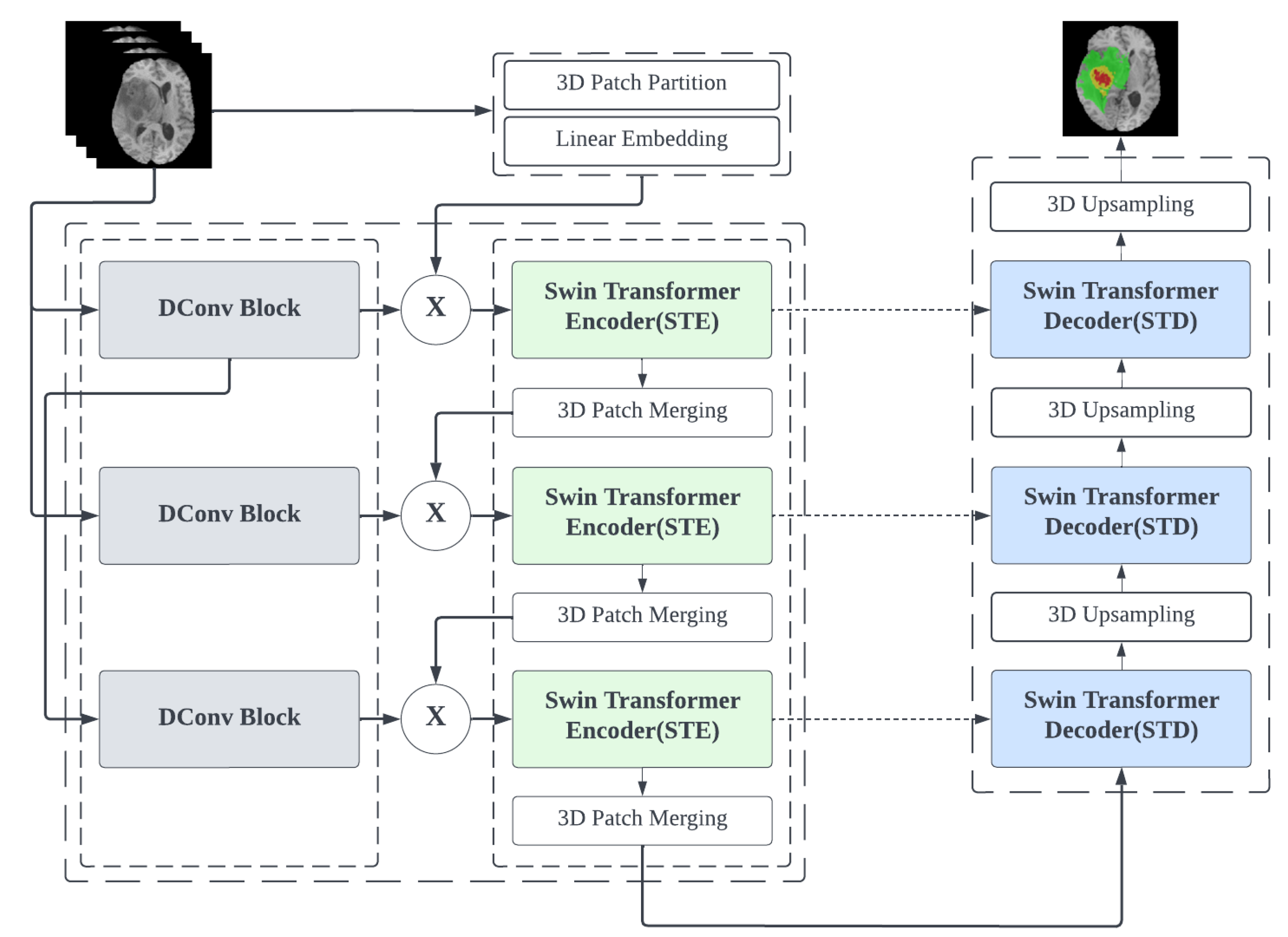
Aiming at solving the above defects relatively, we propose a novel segmentation network with an “encoder–decoder” architecture, namely CSU-Net. The encoder consists of two parallel feature extraction channels based on CNN and Transformer, respectively, in which the features of the same size are fused. The decoder has a dual Swin Transformer decoder block with two learnable parameters for feature upsampling. The features from multiple resolutions in the encoder and decoder are merged via skip connections.
Our main contributions to this work are as follows:
CSU-Net can directly process 3D dataset without slicing each voxel;
CSU-Net proposes a novel architecture in which (1) The encoder structure is based on improved CNN and Swin Transformer in parallel, which enables establishment of remote dependencies at a high level and retains the ability of local feature extraction; (2) The information extracted from the CNN branch is applied in guidance from the following information extraction in the Transformer branch, which can accelerate model convergence and reduce training time; and (3) The decoder structure is based on a dual Swin Transformer parallel structure and introduces two learnable parameters to enhance the capability of restoring information;
We validate the effectiveness of our method on 3D MRI dataset (BraTS). It exceeds the current advanced schemes on WT, ET and TC segmentation regions, to achieve a Dice score of 0.8927, 0.8188 and 0.8857, respectively.
2. Related Work
CNN-based Segmentation Networks: The introduction of CNN has a significant impact on medical segmentation tasks. For 2D segmentation, CE-Net [
14] captures high-level information and preserves spatial information by building a network of contextual encoders. For 3D segmentation, 3D U-Net [
15] is a simple extension of U-Net applied to 3D image segmentation. These networks aim at extracting different dimensions of information during the downsampling process. A deep encoding layer with a smaller receptive field can obtain more accurate edge information. However, these kinds of serial patterns increase the receptive field of the last network layers, leading to incomplete learning of high-level features and inaccurate segmentation of details.
Some networks use parallel structures in the encoder section to increase the information sources or break through the perceptual domain’s limitations. KiU-Net [
16] improves performance by fusing Ki-Net and U-Net to detect smaller perceptual regions. A two-stage multiscale framework proposed by Roth et al. [
17] achieves superior performance in the image segmentation of the pancreas. However, these may lead to inaccuracy of the segmentation due to their poor learning ability in establishing long-distance information transfer dependencies and handling contextual information.
Transformer-based Networks: Vision Transformer has dramatically advanced the performance of machine vision tasks. In ViT [
11], a long-range information model is constructed by transforming images into fixed-size patches and adding positional patch embedding before the sub-attentive mechanism module for more effective global contextual connectivity. Swin-Unet [
18] contains a symmetric encoder–decoder structure using a skip-connection of swin transformer modules, which implements local to global self-attention in the encoder. In its decoder, multiscale features are fused with the encoder using skip-connections. In contrast to Swin-Unet, nnFormer [
19] is computed mainly using a cross-backbone network and a local 3D image block-based self-attention mechanism. They are far less capable of information extraction compared to CNN.
Lin et al. [
20] propose a dual-scale semantic segmentation model based on Swin Transformer to construct long-distance feature relationships between different scales using the self-attention mechanism. It validates the model on several medical datasets, which gains better results. However, adding multiple parallel Swin Transformer channels may increase the amount of model data and computation.
CNN and Transformer Fusion Network: Aiming at the weaknesses of pure CNN networks and pure Transformer networks, the fusion of these two structures can compensate for each other. TransUnet [
21] is the first application of Transformer to CNN, while BiTr-Unet [
22] is also associated with fusing 3D CNN with Transformer. The Transformer block of the above work is performed after the CNN. The features are then recovered by upsampling layer by layer. To achieve accurate image segmentation, image processing requires a large stack of arithmetic power. The overall data volume and computational complexity rise dramatically when dealing with 3D data.
To solve the above problems, we propose a novel parallel network of CNN and Transformer to establish complete global dependencies and preserve the network’s feature extraction ability. The feature extracted by the improved CNN branch is fused with the features of the Swin Transformer and then fed into the next layer of the Swin Transformer module. Throughout the encoding process, the CNN branch uses its powerful feature extraction capabilities to establish guidance for the feature transfer of the Swin Transformer with the different dimensional features.
The key differences between our model and those of other works include the following. (1) CSU-Net is applied to 3D medical images where the network can directly process the volumetric data without needing low-dimensional transformations; (2) CSU-Net uses the improved CNN and Swin Transformer as encoders in parallel, rather than using these encoders in tandem. This parallel structure allows global–local information to be obtained and remains efficient in information processing rates compared to a single deep network.
3. Method
In this section, the overall framework structure of the network is shown first. Then each component, such as DConv, Swin Transformer Encoder and Swin Transformer Decoder, is described in detail.
3.1. Overall Architecture of CSU-Net
This section presents an overview of the proposed CSU-Net model, as shown in
Figure 1.
CSU-Net utilises a parallel architecture which combines CNN and Transformer as an encoder, interacting with the decoder via skip connections. In the parallel architecture, the CNN downsampling channel consists mainly of DConv modules containing large convolutional kernels and bottleneck structures. The Transformer downsampling channel is primarily constructed using Swin Transformer. Considering the possibility of effective parameter loss and inadequate restoration due to dropout in the decoding, we propose a decoder using a dual Swin Transformer block with learnable parameters. In addition, a classification layer is constructed at the end of the overall network to predict the segmentation results. For the BraTS 2020 dataset, three types of segmentation results will be predicted.
3.2. Encoder
3.2.1. Swin Transformer Encoder (STE) Block
The Embedding Block is responsible for converting each input image into non-overlapping patches and subsequently mapping to a tensor of a set dimension. In this design, the patch size is , the sequence length C is set as 96, and then transformed into a high-dimensional tensor .
Swin Transformer has creatively designed a shifted window operation.
Figure 2 shows the Swin Transformer block internal connections and component block.
Each STE (Swin Transformer Encoder) Block consists of a LayerNorm (LN) layer, a multi-head self-attention (MSA) module, a residual connection, and two layers of MLPs containing GELU activation functions. MSA has two kinds of modules: W-MSA (window-based multi-head self-attention) and SW-MSA (shifted window-based multi-head self-attention). In W-MSA, the volume is cut into non-overlapping blocks of a specified size. SW-MSA uses the shifted window mechanism to link unassociated adjacent blocks in W-MSA. The STE Block implements the functions as Equation (
1):
where
l denotes the block layer;
and
denote the output features of the W-MSA module and the MLP module, respectively.
The W-MSA module and SW-MSA module are mainly composed of self-attention mechanisms and trainable relative position encoding. The overall computation is shown in Equation (
2):
where
Q,
K,
V denote the query, key and value, respectively;
denotes the size of the query and key;
B denotes the relative position information deviation value.
To reduce the computational complexity of the attention in 3D images, we build the Sign Transformer Encoder layer by layer using the W-MSA and SW-MSA module and MLP while receiving feature information from the CNN to complement the local attention. The detailed parameters of the STE blocks are shown in
Table 1.
3.2.2. DConv Block
To supplement the information lost in the STE’s downsampling and compensate for the lack of attention to local features, we add a pure convolutional downsampling block, called DConv, to the existing backbone network.
We choose convolutional layers in the parallel network because they encode spatial information at the pixel level, which is more accurate than the patch-level position encoding used in Transformer. Moreover, the convolutional architecture is comparatively lighter while remaining efficient when the computation complexity is caused by shift window operations in existing backbone networks. The original image used three different sizes of 3D convolution kernels. The parameters are shown in
Table 2.
It is worth mentioning that for the third convolution kernel (1, 4, 4), the input does not directly use the original image but the output of the Conv3d_0. This is because the small kernel size helps to reduce the computation complexity compared to the larger kernels while providing the same size perceptual field.
The DConv module consists of the Depthwise Conv, Layer Norm, and GELU. The specific module connections can be found in
Figure 3.
3.2.3. Patch Merging
The primary function of this module is to downsample before moving on to the next STE module. This step can be used to reduce the resolution and, at the same time, adjust the number of channels between each layer, saving some arithmetic. To simplify this process, the patch merging process is conducted using a linear transformation. Elements are selected at regular intervals in multiple directions and expanded after the elements are stitched together to form a complete tensor.
3.3. Decoder
We add a skip connection between the encoder and decoder to transmit the feature representations, which can compensate for the loss of partial information, which is a common defect in a U-shaped network.
Referring to the idea of weighted feature fusion in BiFPN proposed by Tan et al. [
23], we propose the Swin Transformer Decoder(STD) Block. We design the STD block with a learnable parallel structure formed by the multi-head self-attention (MSA) model. The construction is shown in
Figure 4.
Each STD block consists of two identical parallel modules containing W-MSA and SW-MSA. The feature maps from the upper STD block layers are fed into the same two SA modules and subsequently output. When two identical modules fuse, the process is computed as shown in Equation (
3):
where
is the learnable covariate;
l denotes the block layer; F denotes the output of the STD block; X denotes the input of the STD block. In contrast to the single MSA architecture used in Swin-Unet [
18], the present parallel MSA architecture allows increasing self-supervision in the upsampling process. The source of features feeding into the decoder is increased. The possible bias caused by the random dropout in the upsampling process is corrected relatively by the learnable weight variates.
3.4. Classifier Layer
After the decoding session is completed, the classification layer is introduced, and the feature map of depth C is mapped into N categories using a 3D convolutional layer. Thus, the scale of the predicted output is .
3.5. Loss Function
The loss function is a combination of the Dice Loss [
24] and the Binary Cross Entropy Loss. Dice Loss is defined as Equation (
4):
Binary Cross Entropy Loss is defined as Equation (
5):
In Equations (4) and (5), M denotes the number of voxels; N is the number of classes; and denote the probability of output and one-hot-encoded ground truth for class n at voxel m, respectively.
The overall split loss can therefore be defined as Equation (
6):
In Equation (
6), set to a practical value of 0.7.
4. Experiments
In this section, the dataset, the evaluation metrics and other implementation details are described.
4.1. Data and Evaluation Metric
The 3D MRI dataset used in the experiments is provided by the Brain Tumour Segmentation (BraTS) 2020 Challenge [
25,
26,
27]. All samples contained gliomas. Different sequences (T1, T1CE, T2, and FLAIR) were typically generated by various influences on the MR signal, as shown in
Figure 5. These influences can highlight features at different tumour regions to localize the nidus and determine the size of the tumour. The size of each pattern is
. To reduce the effect of unnecessary background on experimental results, all data are cropped to a fixed size of
. Our data preprocessing involves cropping, random rotation and random flipping, which is consistent with baselines. In addition, this dataset consists of relatively high quality MR images. For these two reasons, we do not apply denoising to this dataset.
All four modalities for a sample share the same segmentation file. We aim to output three types of segmentation regions: the Enhancing Tumour (ET): label 1; the Tumour Core (TC): labels 1 and 4; the Whole Tumour (WT): labels 1, 2 and 4.
4.2. Implementation Details
The proposed network implements in PyTorch and trained using an NVIDIA RTX 3090 GPU (24 GB of video memory), using a batch size of 1 and executing 300 epochs from zero. We use the Adam optimizer, with the initial learning rate set to 0.0001. In preliminary tests, training the model directly requires a lot of time, so a pre-trained model is used in this experiment. Swin-T, a model pre-trained in ImageNet-1K by Liu et al. [
28], was used to accelerate the convergence rate of the experiments.
4.3. Evaluation Metrics
We use Dice score and sensitivity to measure the performance of our model.
The Dice score is calculated as Equation (
7):
Sensitivity is an important index in the medical imaging field that can be used to predict the true positive rate of sample images, which can assess the validity and stability of the algorithm model. It is defined as Equation (
8):
In Equations (7) and (8), TP, FP, and FN denote the number of true positives, false positives, and false negatives, respectively.
6. Conclusions
In this paper, we introduce a novel CNN-Transformer-based architecture, dubbed as CSU-Net. It presents a parallel hybrid segmentation framework that effectively fuses 3D Swin Transformer and CNN into the network framework for 3D multimodal brain tumour segmentation in MRI. We proposed to fuse the CNN and Transformer to increase the capability for capturing the global–local information and learning long-range spatial dependencies.
We validated the effectiveness of CSU-Net on the BraTS 2020 dataset. CSU-Net achieves 0.8927, 0.8857, and 0.8188 for the WT, TC, and ET, respectively, outperforming competing methodologies. Our method provides clinical assistance in brain tumour location and diagnosis. However, there exist some shortcomings in our proposed method. Firstly, our test was only performed on BraTS 2020, which lacks promotion in diverse medical images. Secondly, there is still further room to reduce our model’s parameters. We hope to propose a more lightweight Transformer network and work towards developing more efficient medical image segmentation models in future.


