Arc Grounding Fault Monitoring and Fire Prediction Method Based on EEMD and Reconstruction

Abstract

To solve the problem of the single-phase ground fault and occurrence of electrical fires due to the residual current in substation AC power systems, a residual current intelligent sensing technology is proposed based on ensemble empirical modal decomposition (EEMD), sample entropy (SE) reconstruction, and fire warning technology using a beetle antennae search algorithm. First, through the residual current monitoring device to collect residual current information, EEMD and SE reconstruction for arc-earth fault diagnosis and an analysis of the differences in the current characteristics of each line after reconstruction are used to determine the fault line. Second, residual current, temperature, and operating voltage as input parameters and fire probability are the output parameters. The input–output relationship is established by a back-propagation neural network (BPNN) and optimized by the beetle antennae search (BAS) algorithm to speed up the convergence and improve the prediction accuracy to establish a substation fire warning scheme. Through simulation experiments, this paper proposes the residual current as a monitoring object method can effectively diagnose ground faults and accurately predict the probability of fire occurrence to ensure the safe and stable operation of substations.

1. Introduction

A substation station power system is mainly composed of three parts: station AC power system, DC power system, and AC uninterruptible power system [1,2]. Among them, the station AC power system consists of transformers, an AC supply network, transformer power supply, and other parts, and is one of the significant links to ensure the safe and reliable operation of a substation. Station power systems can fail during operation due to mechanical damage, overcurrent, insulation aging, and many other factors that cause grid cables to malfunction [3,4] and cause electrical fires. Among them, the fire caused by insulation damages the creep age arc. Due to arc impedance, the arc fault current is small, cannot be protected by short circuit protection, and the residual current device is needed for electrical fire protection [5].

For the grounding fault of the substation transmission line caused by the fault current, the decomposition of the current signal can effectively extract fault characteristics and judge the fault line. Reference [6] proposes a grounding fault line selection method based on wavelet packet decomposition, which decomposes the zero-sequence current into multiple components through a wavelet packet to select the fault line. Reference [7] applies empirical mode decomposition (EMD) to the fault location of the offshore wind power system. Through the EMD decomposition and extraction of the inherent mode function (IMF) generated in the signal, the Hilbert transform is used to evaluate the fault location target, and the effectiveness of the proposed method is verified by comparison with the wavelet transform. However, WPD needs to set the decomposition parameters in advance, and EMD has the problem of modal aliasing in the decomposition process. Ensemble empirical mode decomposition (EEMD) can solve the above problems and has been widely used in time series prediction, fault feature extraction, distribution network fault location, and so on [8,9,10]. In this study, EEMD is used to analyze the residual current, extract the fault characteristics of the fault current, and judge the fault line. Combined with the residual current monitoring device, the AC power supply grounding fault monitoring can be realized.

An AC power system has a large number of cables, which are distributed in cable trays and cable shafts. If it is in the fault state for a long time, the high temperature generated by the fault current will lead to cable fire and cause severe losses. Therefore, it is necessary to predict the probability of fire. Reference [11] uses the back-propagation neural network (BPNN) to predict open flame probability, smoldering probability, and no fire probability and takes smoke concentration, CO concentration, and temperature as input variables. Reference [12] applies multi-information fusion and BPNN to building fire alarms, taking smoke concentration, CO concentration, and temperature as input signals. The actual fire probability is basically consistent with the expected fire probability, which is conducive to fire detection. However, BPNN randomly selects weights and thresholds in the prediction process, which will lead to slow convergence and fall into optimal local values. Reference [13] uses the genetic algorithm (GA) to optimize the weight and threshold of BPNN for predicting the fire risk index. The results show that GA-BP significantly improves prediction accuracy. Similar methods include particle swarm optimization (PSO) and other methods [14]. Although the above method optimizes the parameters of BPNN, GA has a high complexity, and the PSO algorithm has a slow convergence speed [15]. The beetle antennae search (BAS) algorithm is a heuristic search algorithm inspired by the beetle’s predatory behavior. The algorithm has good global search ability and convergence. According to the adaptive step size, it can effectively jump out of the optimal local value in the early exploration stage and quickly converge at the end of the search [16]. At present, it has been applied in a variety of industrial engineering applications. Reference [17] applies the BAS algorithm to a rolling bearing diagnosis and combines it with a deep learning method to improve fault diagnosis performance. Reference [18] proposed a multi-factor gas explosion pressure prediction model based on BAS-BP, which considers gas, ignition, and other factors and can predict more accurately than traditional methods. This study proposes to use BAS to optimize BPNN and apply the BAS-BP model to fire probability prediction.

Therefore, this study takes the residual current as the monitoring object, designs the residual current decomposition method of EEMD-SE, and solves the problem of parameter setting of WT and EMD mode aliasing. The entropy value of the IMF component is calculated by SE and reconstructed to reduce the number of components and better extract the characteristics of the fault current signal to diagnose the fault line. For a fire caused by fault current, the residual current and temperature are taken as the research objects, and a prediction model based on BPNN is proposed. The weight and threshold of BPNN are optimized by the BAS algorithm, which improves the speed of fire probability prediction and the accuracy of the results. The main innovations of this study are as follows:

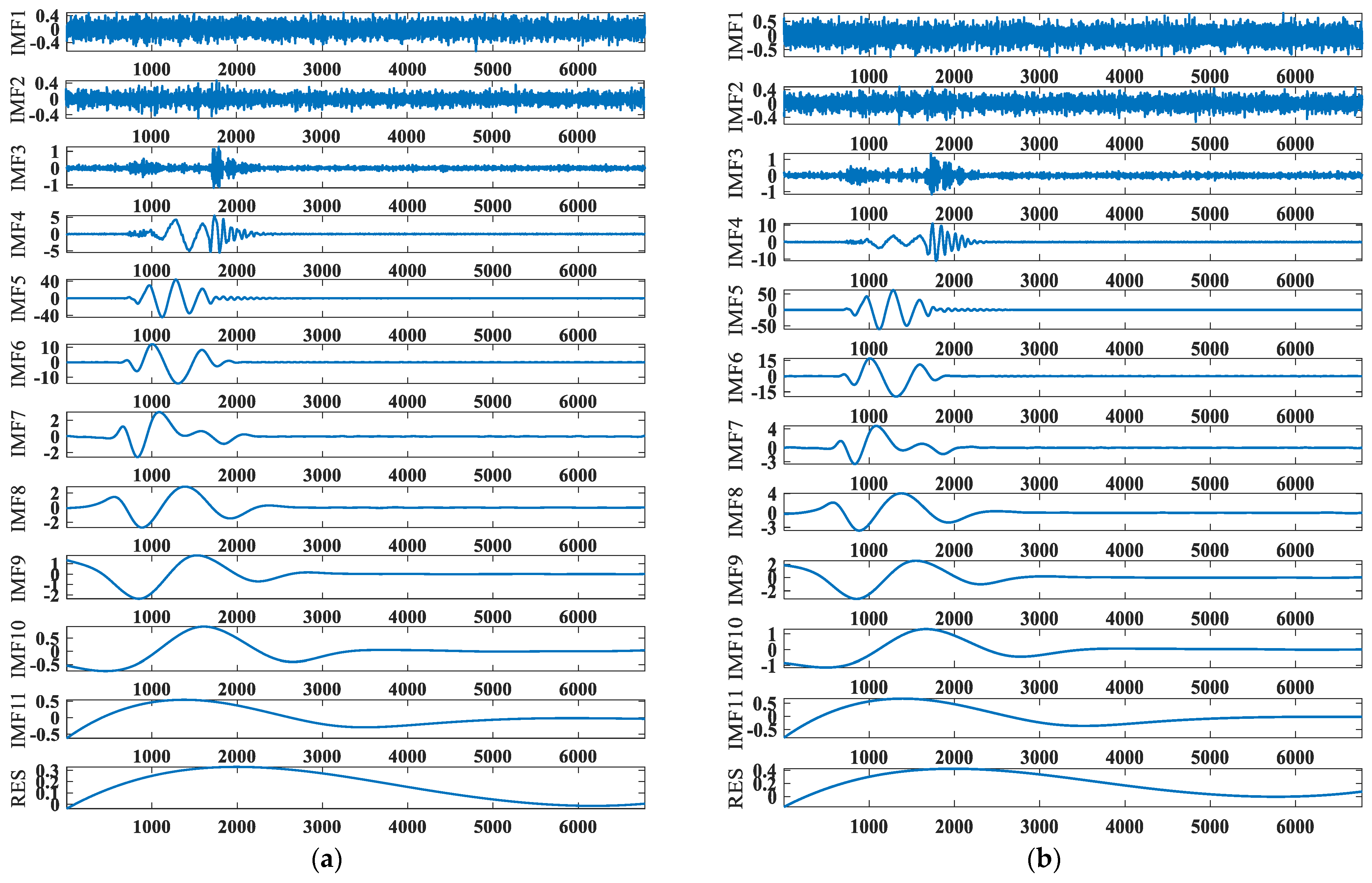
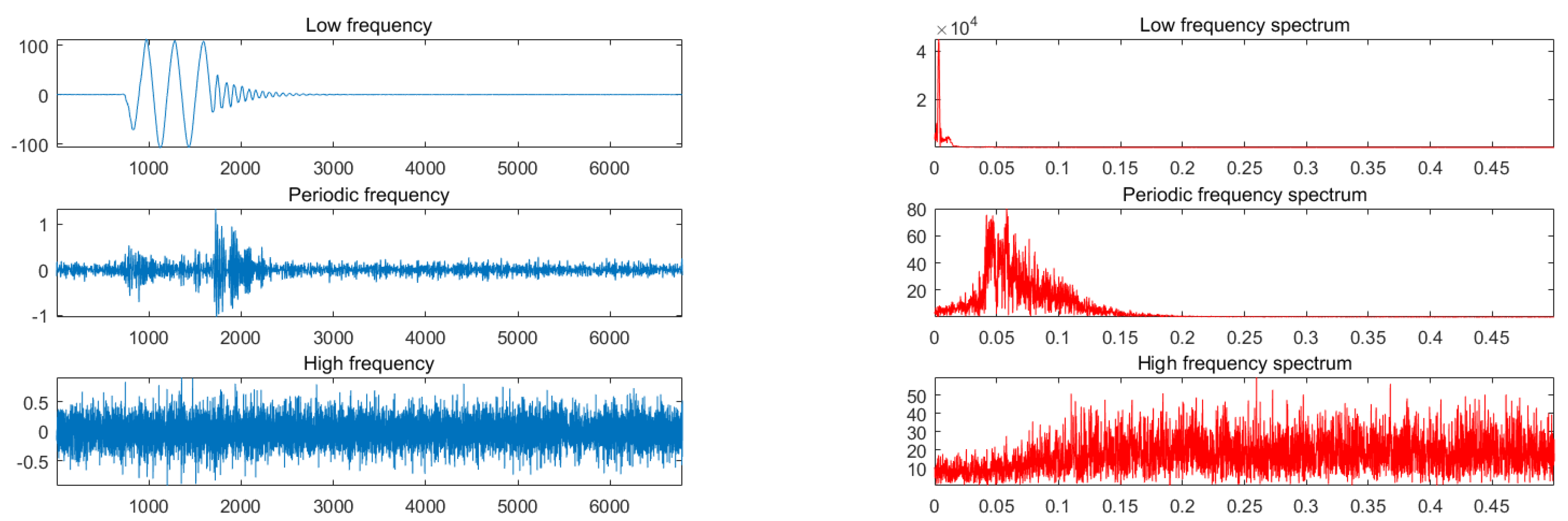
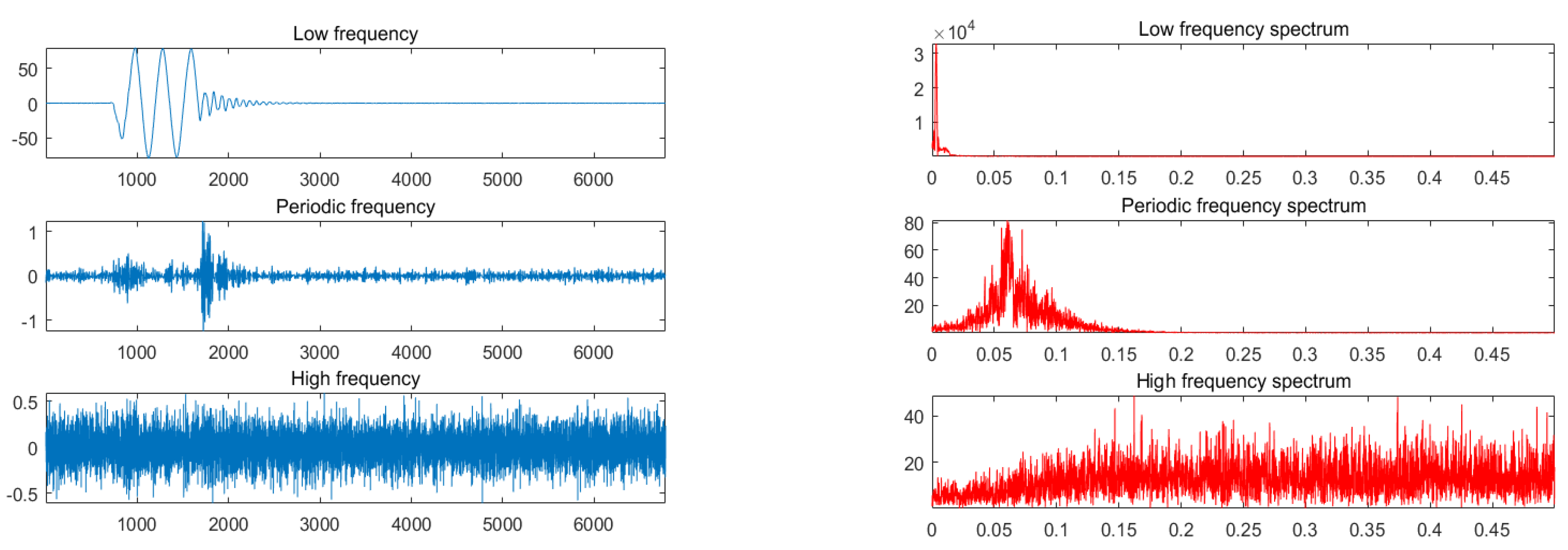
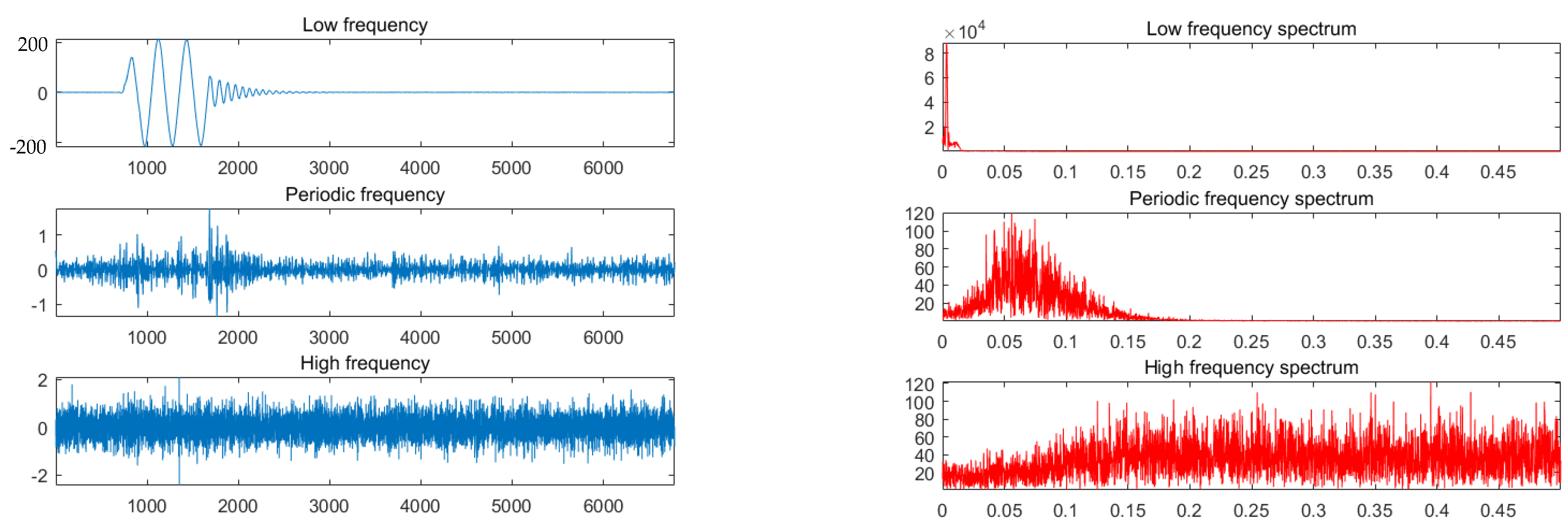
• Through monitoring the residual current, the EEMD is used to decompose the current, calculate the entropy of the IMF component and reconstruct it, remove the redundant information, and analyze the difference between the fault line and the normal line according to the reconstructed signal.
• Residual current is selected as the input of BPNN and applied to fire probability prediction. Aiming at the problems of slow convergence speed and easily falling into the optimal local value of the BP algorithm, the BAS algorithm is proposed to optimize the weight and threshold of BPNN.
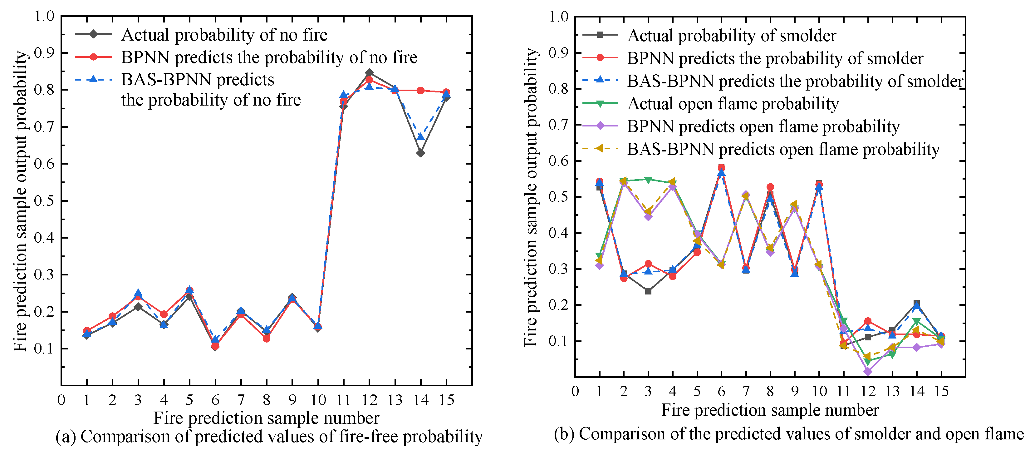
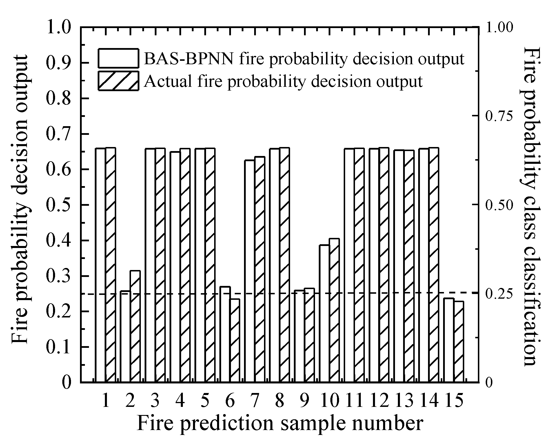
• Simulation verification. The fault line is judged by analyzing the reconstructed signal’s characteristics. BAS-BP is compared with BPNN, and the model’s performance is evaluated according to the probability of fire occurrence.

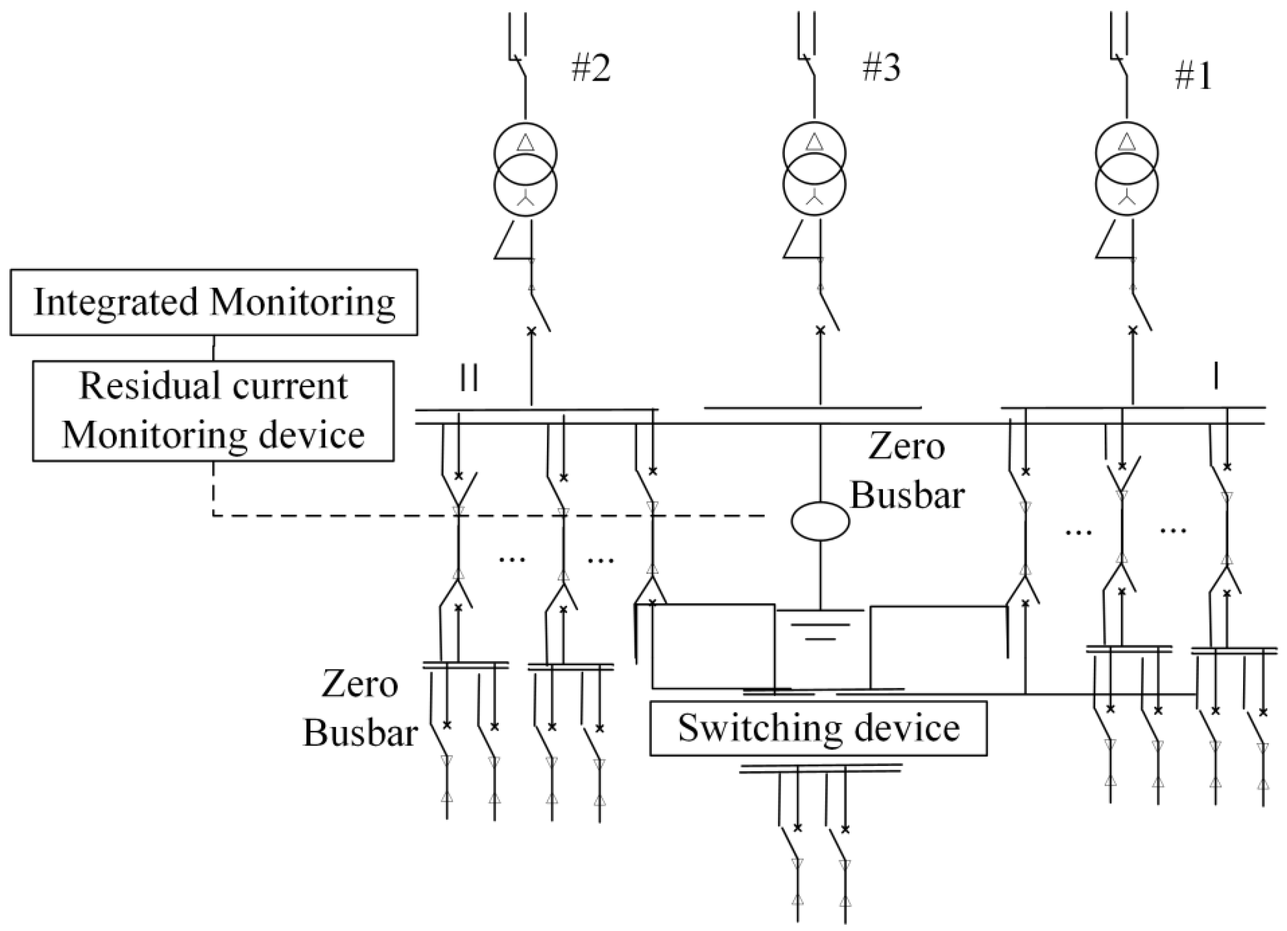
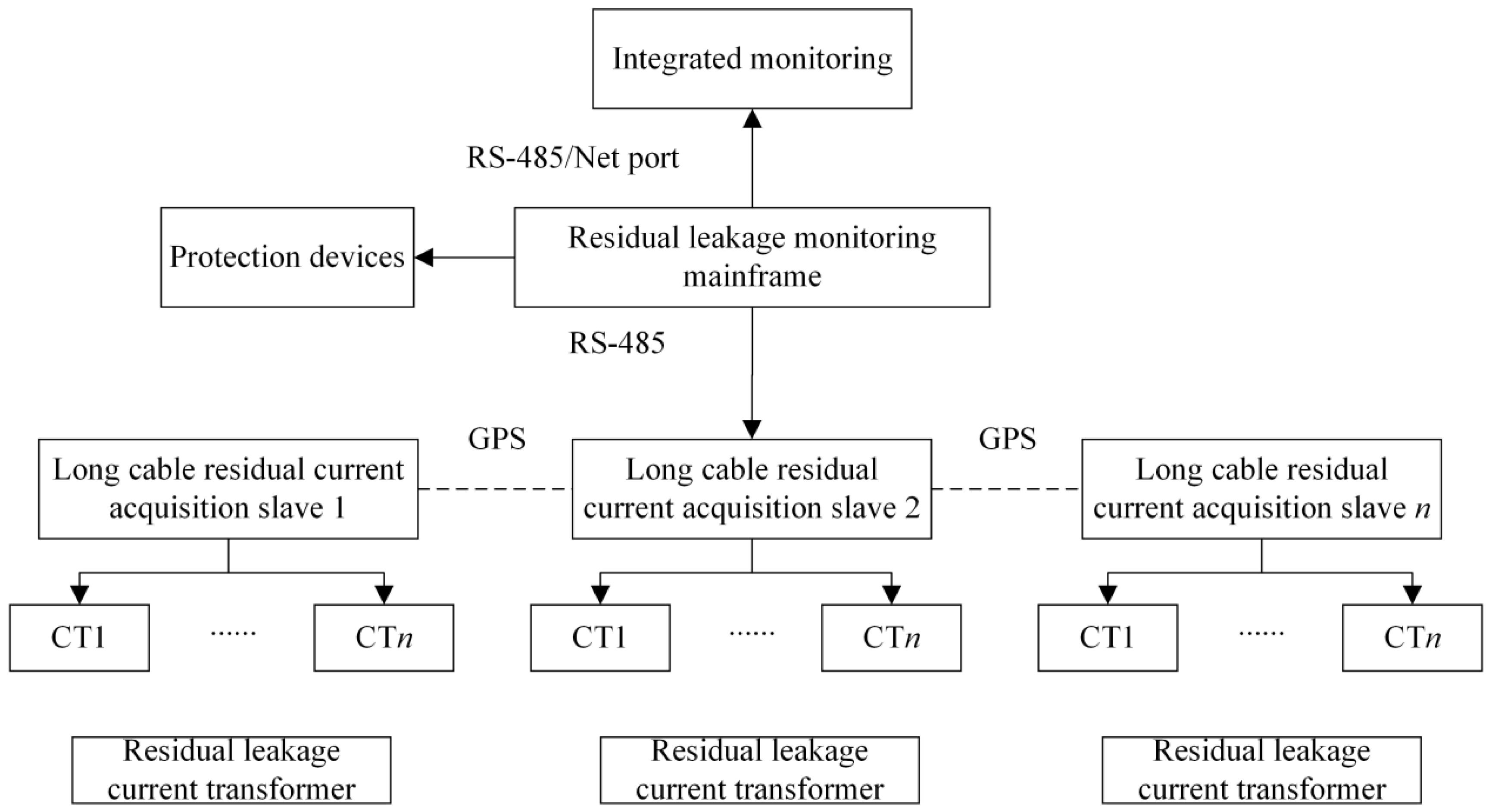
2. Residual Current Monitoring

For residual current, also known as leakage current, with normal use of the low-voltage distribution system, the current vector sum of phases A, B, C, and N is in balance. When a fault occurs, the balance breaks, and the current vector sum is not 0. Generally, the fault usually occurs at the power consumption side because the fault causes the incoming and outgoing current of the primary circuit to no longer maintain balance, and a current instantaneous vector practical value, namely residual current, will be formed. Residual currents are generated for many reasons, such as the long-term use of the connecting conductor, resulting in aging and breakage; construction irregularities; irregular design; and failure to change the line as required [19].

As one of the important causes of electrical fires, the generation of leakage current destroys the protection device of the equipment; failing insulation protection, the leakage current itself is not the direct cause of the fire. However, when the leakage current occurs, the fire line is connected to the earth to produce a larger current, according to the thermal effect, generating much heat and igniting combustible materials, resulting in fire occurrence. An electrical fire caused by leakage current is hidden and not easily found, which is very dangerous.

Monitoring residual current has become an effective means of the early prevention and control of electrical fires to better monitor the residual current and obtain timely and accurate electrical data. This paper establishes a residual current monitoring scheme. Through a residual leakage current transformer (CT), combined with a GPS positioning system, data are transmitted to the protection device and the integrated monitoring unit in real-time, achieving real-time transmission, early warning, early action, etc. [20,21]. The residual current monitoring scheme is as follows (See Figure 1 for details).

3. Research on AC Power Ground Fault in Substations

3.1. Station AC Power Ground Fault Intelligent Sensing Technology

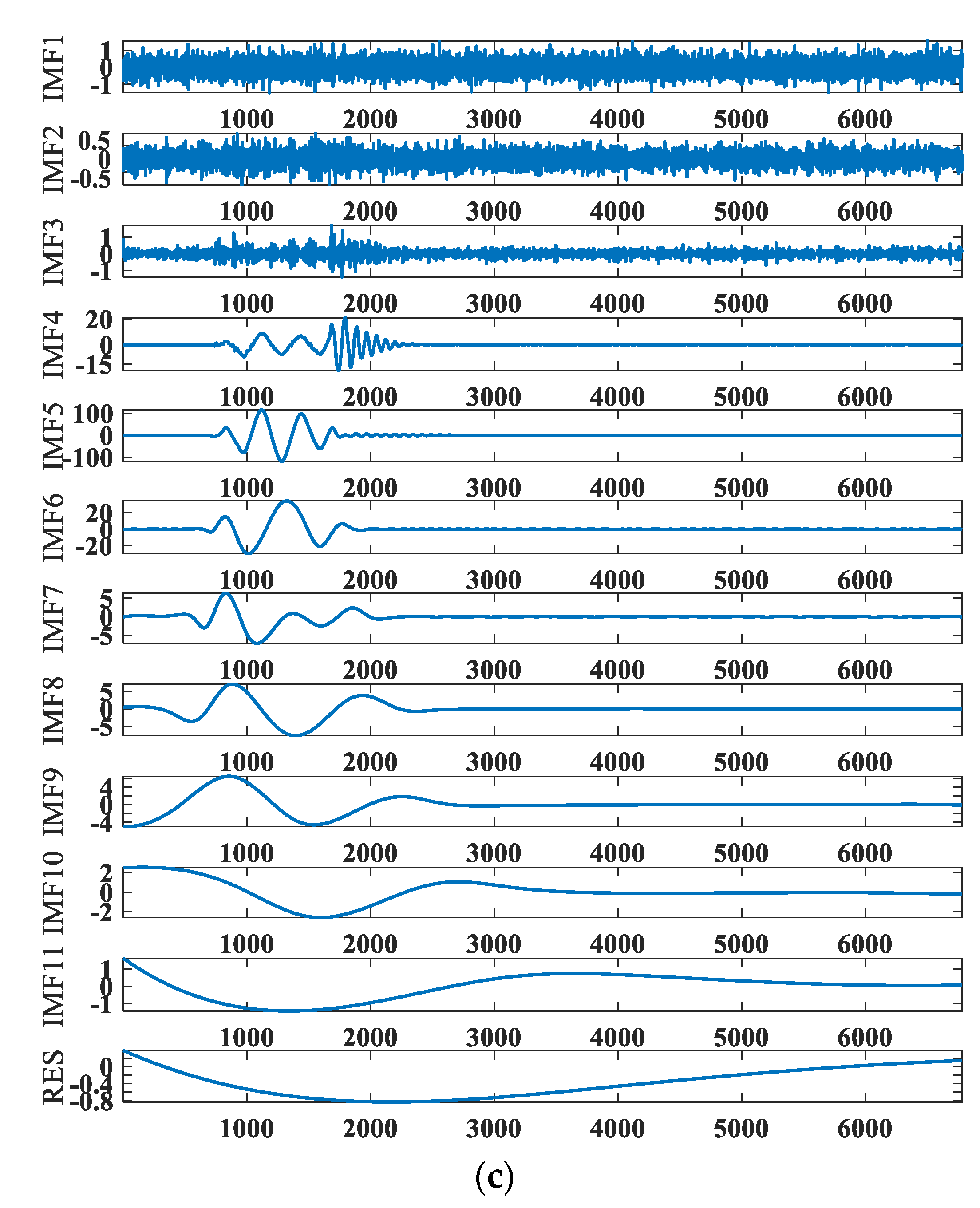
The arc grounding fault diagnosis technology forms a station AC power grounding fault-sensing technology system by the online monitoring of the AC power residual current through the wavelet decomposition method. As in Figure 2, the cable operation condition is analyzed through a residual current monitoring device. The pure signal is extracted by filtering and separation mainly through wavelet decomposition, and the wavelet decomposition method is used to characterize the monitoring data.

3.2. EEMD

Empirical mode decomposition (EMD), which can decompose any complex signal into multiple intrinsic mode functions (IMF), can be used to analyze time series.

The EMD decomposition steps are as follows:

• Identify all maxima and minima and fit their envelopes, e_up(t) and e_low(t), and calculate the average value of the upper and lower envelopes m₁(t).

  $$m_1(t)=\frac{e_{up}(t)-e_{low}(t)}{2}$$

  (1)
• The IMF component c₁(t) is removed from the original signal to extract the residual component,

  $$r_1(t)=x(t)-c_1(t)$$

  (2)

However, the above algorithms introduce the modal aliasing problem when processing signals with abrupt changes in time scales. EEMD can effectively improve the modal aliasing problem by adding Gaussian white noise to the original signal and then performing multiple EMDs to define the overall averaging of the decomposed IMF components [22,23].

The specific decomposition steps of the EEMD method are:

• Add a random Gaussian white noise sequence to the target signal:

  $$x_l(t)=x(t)+n_l(t)$$

  (3)

In the lth experiment, n_l(t) is the white noise sequence with an added standard normal distribution.

2.

Decomposition of the signal using EMD to obtain n IMF components and 1 RES component.

$$x_l(t)={\displaystyle \sum _{i=1}^n{c}_{li}(t)+r_l(t)}$$

(4)

3.

Repeat the above steps by adding a different sequence of white noise each time.

4.

Using the characteristic that the white noise spectrum has zero mean, the above components are averaged to obtain the final decomposition results as follows:

$$\{\begin{array}{l}{c}_i(t)=\frac{1}{N}{\displaystyle \sum _{l=1}^N{c}_{li}(t)}\\ r(t)=\frac{1}{N}{\displaystyle \sum _{l=1}^N{r}_l(t)}\end{array}$$

(5)

where: N is the number of times white noise is added; c_i(t) is the i-th IMF component after integrated averaging; and r(t) is the final residual component.

3.3. SE

Entropy is a quantitative descriptive tool to measure the complexity of a system, and the entropy value varies with the system’s state. The sample entropy value’s magnitude accurately reflects the time series’ complexity [24]. The steps to calculate the sample entropy are as follows:

• Time series $\left\{x_i\right\}=\left\{x_1,x_2,\dots ,x_N\right\}$ form the series into an m-dimensional vector according to the ordinal number:

  $$X_i=\left[x_i,x_{i+1},\dots ,x_{i+m-1}\right],(i=1,2,\dots ,N-m+1)$$

  (6)
• Ascertain distance between the vectors X(i) and X(j); $d_m[X(i),X(j)]$ is the absolute value of the maximum difference between the two corresponding elements.

  $$d_m[X(i),X(j)]=\underset{0\sim m-1}{\max }[\left|x(i+k)-x(j+k)\right|]$$

  (7)
• Given the similarity tolerance r, for each value of the i statistics number of $d[X_m(i),X_m(j)]<r$, denoted as B_m(i), calculate the ratio to a total number of distances N-m, denoted as $B_i^m(r)$. Definition:

  $$B_i^m(r)=\frac{B_m(i)}{N-m},1\le i\le N-m,i\ne j$$

  (8)
• Find the average of all $B_i^m(r)$ and denote as $B^m(r)$, then

  $$B^m(r)=\frac{1}{N-m+1}{\displaystyle \sum _{i=1}^{N-m+1}{B}_i^m(r)}$$

  (9)
• Update m to m + 1 and repeat the above steps, noting as $B^{m+1}(r)$

  $$B^{m+1}(r)=\frac{1}{N-m}{\displaystyle \sum _{i=1}^{N-m}{B}_i^{m+1}(r)}$$

  (10)
• SE is

  $$\mathrm{Samp} \mathrm{En}(m,r)=\underset{N\to \infty }{\lim }\left\{-\ln \left(\frac{B^{m+1}(r)}{B^m(r)}\right)\right\}$$

  (11)

When N is a finite value, the estimate of SE is

$$\mathrm{Samp} \mathrm{En}(m,r,N)=-\ln \left(\frac{B^{m+1}(r)}{B^m(r)}\right)$$

(12)

In text, take m = 2, r = 0.2 Std.

4. Substation Fire Warning Method Research

This paper sets the residual current, temperature, and operating voltage as the input signals. The BPNN is used to output no fire’s probability, smolder’s probability, and open flame’s probability to determine the fire situation of a substation. The BPNN is divided into an input layer, implicit layer, and output layer, and gradient descent is used to realize the algorithm’s operation by quickly calculating the function’s derivative. The BPNN that falls into local optimum is easy; for a prediction to solve the above problems, the BAS algorithm is introduced for optimization.

4.1. Establishing Input and Output Relationships

The input signal is set to X_i, where i = 1, 2, …, n. The output signal is set to Y_j, j = 1, 2, …, m. The relationship is expressed as

$$S_k={\displaystyle \sum _{i=1}^n{v}_{ki}{X}_i+v_{k0},1\le k\le h}$$

(13)

$$Z_k=\sigma (S_k),1\le k\le h$$

(14)

$$Y_j={\displaystyle \sum _{k=1}^h{w}_{jk}{Z}_k+w_{j0},1\le j\le m}$$

(15)

For reverse pass error, update modification weights v_ki and v_k0, and threshold w_jk and w_j0, until the requirement is satisfied, the error function is

$$E=\frac{1}{2}{\displaystyle \sum _{a=1}^t{\displaystyle \sum _{k=1}^m{(q_k^a-p_k^a)}^2}}$$

(16)

where $q_k^a$ is the actual output, and $p_k^a$ is the desired output.

4.2. BAS Algorithm

The BAS algorithm is mainly developed based on the actual situation of the aspen foraging learning summary, and aspen whiskers are the primary tool for aspen to hunt and feed. The left and right aspen whiskers make judgments based on food smell and perform the corresponding actions to hunt. According to the foraging behavior of the aspen, it can be seen that the aspen whisker search algorithm can avoid the local optimum.

The BAS process is:

• Set up random variables and normalize them:

  $$\overrightarrow{b}=\frac{rand(k,1)}{\Vert rands(k,1)\Vert }$$

  (17)

The rand is a random function; ‖rand‖ indicates the spatial dimension.

2.

Create spatial coordinates:

$$\{\begin{array}{l}{x}_{lt}=x_t-\frac{d_0\ast \overrightarrow{b}}{2}\\ x_{rt}=x_t-\frac{d_0\ast \overrightarrow{b}}{2}\end{array}$$

(18)

The intensity of the food odor received by the left and right whiskers is calculated using the adapted function f(x).

3.

Location update:

$$x_{t+1}=x_t-sign(f(x_{rt})-f(x_{lt})){\delta }_t\ast \overrightarrow{b}$$

(19)

4.3. Optimized Prediction Model Based on BAS-BPNN Algorithm

Due to the randomness of the initial threshold and weight selection, the convergence times are different, and even the standard error cannot be reached within the specified times. BPNN is optimized using the BAS algorithm. The BAS-BP process is:

• Random vectors of beetle antennae are created and normalized;
• The left and right spatial coordinates of longicorn whiskers are obtained. According to the fitness function f(x), determine the strength of the food odor be obtained from the left and right, judge the moving direction of the longicorn beetle, and update the position of the longicorn beetle;
• Select step factor δ^t. It is mainly used to control the area search ability of beetles; select a more significant value as much as possible to avoid falling into local optimization. The step factor changes dynamically with time;

  $${\delta }^{t+1}={\delta }^t\cdot eta$$

  (20)

The formula: eta is the step attenuation factor, and the value range is [0, 1];

4.

Assuming the initial value, calculate the fitness function value, and store the current initial position of the bestX and the corresponding fitness function value bestY;

5.

Calculate the length of beetle antennae and build a search space. The position of beetle antennae that must receive information updates through beetle antennae, the fitness function, calculates the second fitness function value, compares it with bestY, determines the current optimal fitness value, and saves the corresponding weight as the current optimal weight;

6.

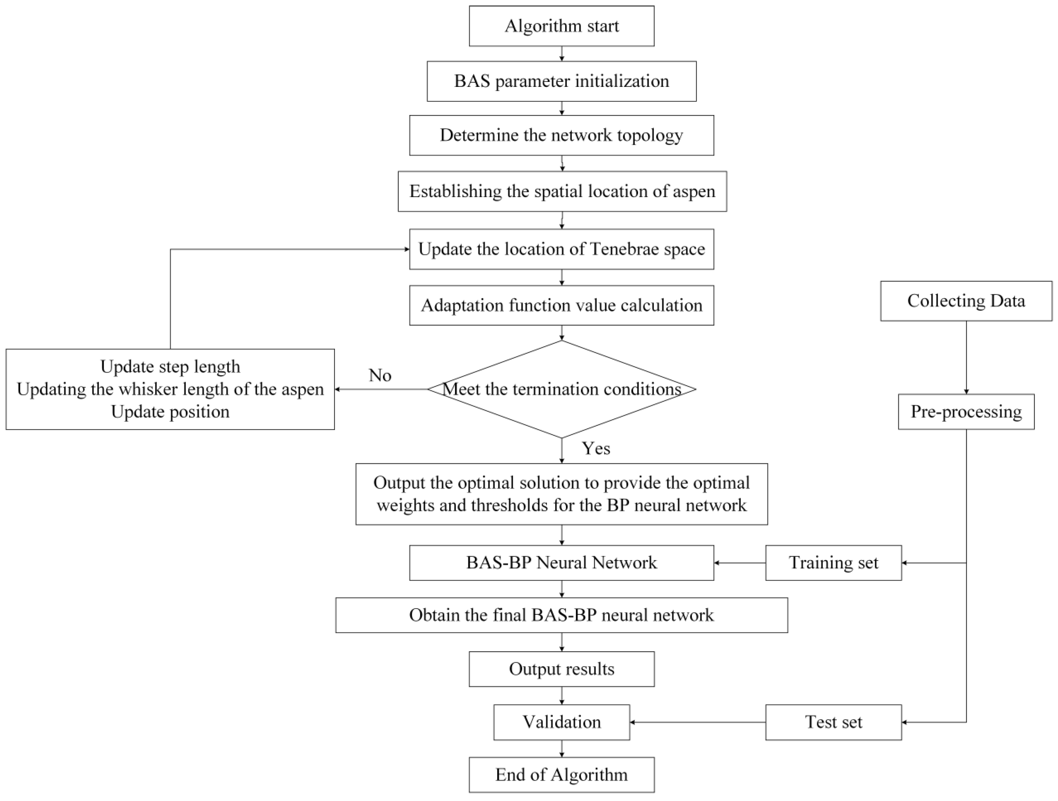
Test the termination condition of the algorithm. If the conditions are met, the algorithm will jump out. Otherwise, a new round of optimization will be carried out. Figure 3 is the flow chart of the BAS-BP algorithm.

5. Case Study

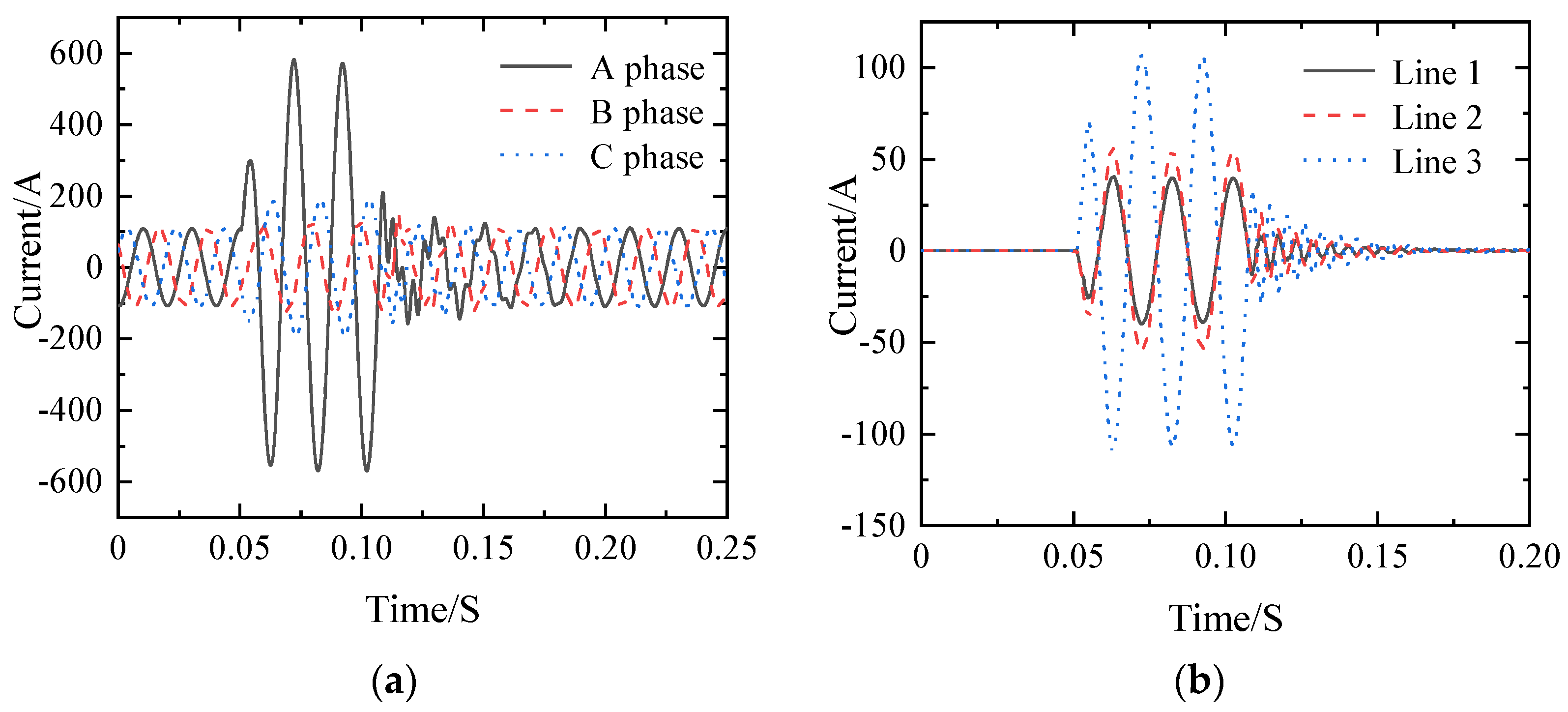
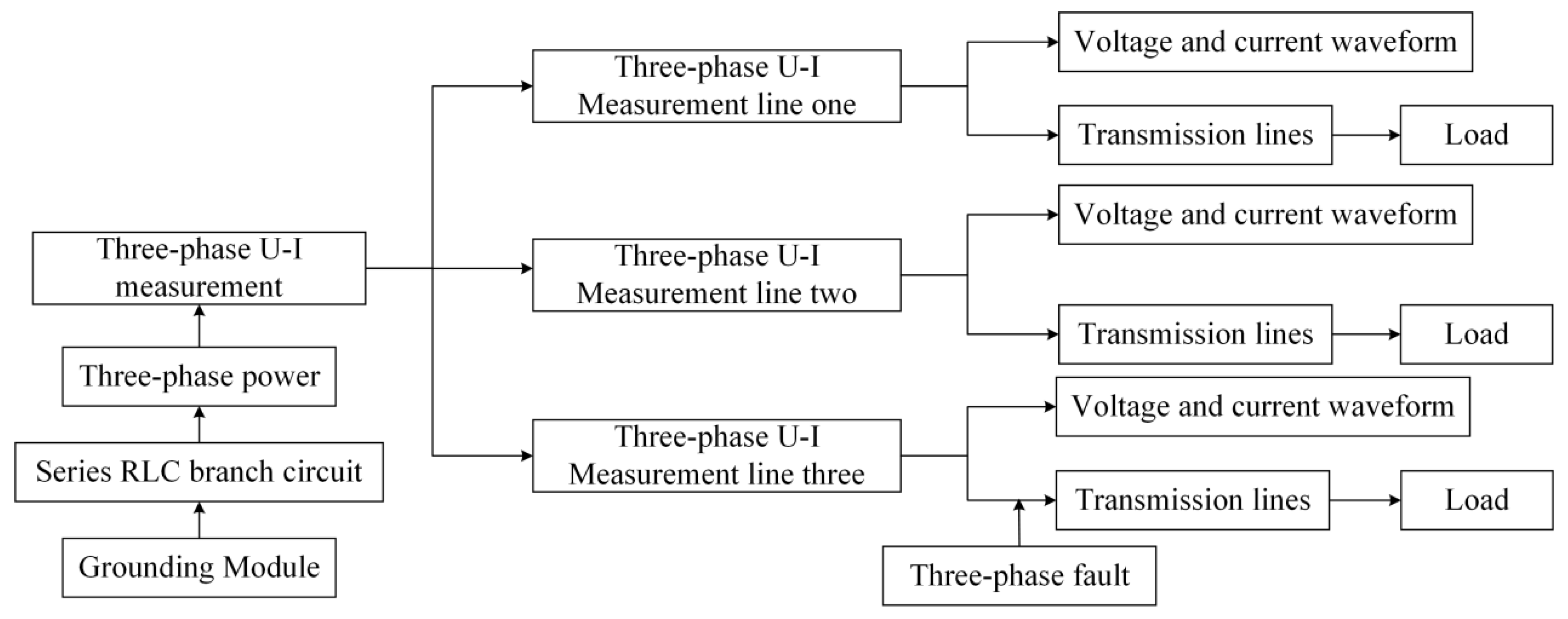
5.1. Grounding Fault Simulation Analysis

A single-phase ground fault simulation model is built, as show in Figure 4. After obtaining the waveform signal of each line, the current waveform is decomposed by EEMD, and the A-phase ground fault occurs in Line 3 at 0.05 s.

According to the results in Figure 5, before 0.05 s, the three lines are normal, and the zero-sequence current of each line is zero. At 0.05 s, the third line suddenly produces an A-phase arc grounding fault.

EEMD decomposes the zero sequences current waveform. The EEMD results show that the frequency domain signal direction of the fault line is different from the direction of the first two lines, and the current amplitude of the ground fault line is larger. The fault line can be found by comparing the difference between the normal line and the abnormal line. After calculating the signal energy proportion after EEMD decomposition, it is found that the proportion of the 0–8 Hz frequency range is high so that fault analysis can be carried out according to the signals in this range.

This paper sets the grounding resistance of 100 Ω, and the current signal after EEMD decomposition is reconstructed. The comparison of decomposition waveforms of the 100 Ω normal line and fault line is shown in Figure 6.

The sample entropy values calculated for each line are shown in

Table 1. Sample entropy values for different line components.

	IMF1	IMF2	IMF3	IMF4	IMF5	IMF6	IMF7	IMF8	IMF9	IMF10	IMF11	RES
Line 1	2.0726	1.4908	0.5703	0.0154	0.0068	0.0027	0.0032	0.0025	0.0021	0.0014	0.0025	0.0018
Line 2	2.0682	1.5051	0.5863	0.0128	0.0070	0.0023	0.0032	0.0025	0.0019	0.0015	0.0025	0.0022
Line 3	2.0638	1.4853	0.6760	0.0098	0.0053	0.0024	0.0039	0.0026	0.0017	0.0015	0.0026	0.0021

.

According to the sample entropy value, the decomposed waveform is reconstructed (See Figure 7, Figure 8 and Figure 9 for details). Comparing the amplitude and polarity of the reconstructed signals in different frequency bands, the faulty line can be judged, where the normal line polarity is negative and the faulty line polarity is positive. It can be judged that the line is faulty, which is consistent with the setting of the faulty line in the simulation model.

The reconstructed signal and spectrum of different lines are analyzed. The low-frequency components of the fault line and the normal line change differently. The changing amplitude of the periodic frequency component of the faulty line is greater than that of the normal line at the beginning of the fault. The spectrum of the periodic frequency component of the faulty line is also different from the normal line. Based on the above, the analysis can determine line three for the fault signal.

5.2. Substation Fire Probability Prediction

The input and output signals are 3, the implied layer nodes are set to 6, the learning speed is 0.01, the maximum training times are 5000, and the MSE is 0.0001. The predicted probability of substation fire using the trained BAS-BP model is shown in Figure 10.

From the analysis in Figure 10, the fire probability error predicted by BAS-BPNN is significantly better than that of BPNN.

Two error indicators evaluate the accuracy of the substation fire warning model, the Y_MAPE and Y_RMSE. The smaller the error, the more accurate the substation fire prediction model, and the two error calculation formulas are shown:

$$Y_{MAPE}=\frac{100\%}{n}{\displaystyle \sum _{i=1}^n\left|\frac{y_a(i)-y_p(i)}{y_a(i)}\right|}$$

(21)

$$Y_{RMSE}=\sqrt{\frac{{{\displaystyle \sum _{i=1}^n\left[\frac{y_a(i)-y_p(i)}{y_a(i)}\right]}}^2}{n}}$$

(22)

where n denotes the total number of predicted results, and y_a(i) and y_p(i) are the actual and predicted values of fire probability for the i-th test point. The RMSE and MAPE of the BAS-BPNN algorithm and BPNN algorithm are shown in

Table 2. Comparison of fire probability error between two algorithms.

Algorithm	RMSE			MAPE/%
	No Fire	Smolder	Open Flame	No Fire	Smolder	Open Flame
BP	0.046	0.034	0.036	7.7	11.1	13.5
BAS-BP	0.021	0.020	0.032	4.8	8.53	10.8

.

As analyzed in Table 2, MAPE decreased by 37.66% and RMSE decreased by 54.35% for the probability of no fire, MAPE decreased by 23.15% and RMSE decreased by 41.18% for the probability of cloudy combustion, and MAPE decreased by 20% and RMSE decreased by 11.11% for the probability of an open fire.

The fuzzy algorithm analyzes the output fire probability. The fire duration factor is added to classify the decision output value u into four levels. When u < 0.25 is no fire, 0.25 ≤ u < 0.5 is alert, 0.5 ≤ u < 0.75 is the alarm, and u ≥ 0.75 is a serious alarm. A comparison of fire probability output after processing by the fuzzy algorithm is shown in Figure 11.

As seen from the analysis of Figure 11, the fire probability after processing by the fuzzy algorithm, BAS-BP prediction is the same as the actual; only the sixth fire test point is different, BAS-BP judged as alert, and the actual situation is no fire. The reason for this may be that the fire duration is set too long, and the training data is small. In order to reduce the error, more data are needed to train the prediction model in the future.

6. Conclusions

In this study, residual current is taken as the research object, and a fault line judgment method based on EEMD-SE and a fire probability prediction model based on BAS-BP are proposed. The EEMD method avoids the problem of setting parameters in advance of WT and solves the problem of the modal aliasing of EMD. By decomposing and reconstructing the residual current signal, the difference between the fault line and the normal line can be better analyzed through simulation experiments, which provide a reference for AC power supply grounding fault line selection. Aiming at fires caused by residual current, residual current and temperature are the main factors affecting fire probability. The influencing factors, such as smoke concentration and CO concentration, are removed. The probability of fire occurrence is predicted in advance by BPNN. A BAS algorithm is used to optimize the weight and threshold of BPNN, which further improves the prediction accuracy and can more accurately judge whether a fire occurs. In the following work, the combination of grounding fault line selection and artificial intelligence technology, as well as the collaborative work of fire probability prediction and fire protection devices, will be some of the research focuses.

References

1. Zhang, Z.Y.; Wang, Z.Y.; Kang, C.; Yu, F.; Ma, Z.X.; Gou, J. Research on overvoltage characteristics and influencing factors of converter station under grounding fault. Energy Rep. 2022, 8, 445–454. [Google Scholar] [CrossRef]
2. Salvadori, F.; Gehrke, C.S.; Hartmann, L.V.; Freitas, I.S.; Santos, T.d.S.; Texeira, T.A. Design and implementation of a flexible intelligent electronic device for smart grid applications. In Proceedings of the 2017 IEEE Industry Applications Society Annual Meeting, Cincinnati, OH, USA, 1–5 October 2017; pp. 1–6. [Google Scholar]
3. Courty, L.; Garo, J.P. External heating of electrical cables and auto-ignition investigation. J. Hazard. Mater. 2017, 321, 528–536. [Google Scholar] [CrossRef] [PubMed]
4. Liang, X.M.; Zhang, P.; Chang, Y. Recent advances in high-voltage direct-current power transmission and its developing potential. Power Syst. Technol. 2012, 36, 1–9. [Google Scholar]
5. Park, D.; Kim, I.; Choi, S.; Kil, G. Detection algorithm of series arc for electrical fire prediction. In Proceedings of the 2008 International Conference on Condition Monitoring and Diagnosis, Beijing, China, 21–24 April 2008; pp. 716–719. [Google Scholar]
6. Zhao, J.W.; Lou, J.N.; Sun, J.; Feng, Z.X.; Li, P.; Gao, M.M. A new method for faulty line selection in distribution systems based on wavelet packet decomposition and signal distance. In Proceedings of the 2019 IEEE 8th International Conference on Advanced Power System Automation and Protection, Xi’an, China, 21–24 October 2019; pp. 596–600. [Google Scholar]
7. Perveen, R.; Mohanty, S.R.; Kishor, N. Fault location in VSC-HVDC section for grid integrated offshore wind farm by EMD. In Proceedings of the 2016 18th Mediterranean Electrotechnical Conference, Lemesos, Cyprus, 18–20 April 2016; pp. 1–5. [Google Scholar]
8. Zhang, G.D.; Zhou, H.M.; Wang, C.J.; Xue, H.Z.; Wang, J.D.; Wan, H.W. Forecasting time series albedo using NARnet based on EEMD decomposition. IEEE Trans. Geosci. Remote Sens. 2020, 58, 3544–3557. [Google Scholar] [CrossRef]
9. Gao, K.P.; Xu, X.X.; Li, J.B.; Jiao, S.J.; Shi, N. Weak fault feature extraction for polycrystalline diamond compact bit based on ensemble empirical mode decomposition and adaptive stochastic resonance. Measurement 2021, 178, 109304. [Google Scholar] [CrossRef]
10. Xue, S.Z.; Cheng, X.G.; Lv, Y.X. High resistance fault location of distribution network based on EEMD. In Proceedings of the 2017 9th International Conference on Intelligent Human-Machine Systems and Cybernetics, Hangzhou, China, 26–27 August 2017; pp. 322–326. [Google Scholar]
11. Yun, Y. Situation Prediction of Fire Management System Based on BP Neural Network. In Proceedings of the 2021 11th International Conference on Information Technology in Medicine and Education, Wuyishan, China, 19–21 November 2021; pp. 174–179. [Google Scholar]
12. Zhang, W. Electric fire early warning system of gymnasium building based on multi-sensor data fusion technology. In Proceedings of the 2021 International Conference on Machine Learning and Intelligent Systems Engineering, Chongqing, China, 9–11 July 2021; pp. 339–343. [Google Scholar]
13. Chen, L.; Wang, Y.Q. Research on the material fire risk index based on the GA-BP neural network. In Proceedings of the 2021 International Conference on Advances in Optics and Computational Sciences, Ottawa, OT, Canada, 21–23 January 2021; pp. 1–6. [Google Scholar]
14. Zhang, Y.X.; Cui, N.B.; Feng, Y.; Gong, D.Z.; Hu, X.T. Comparison of BP, PSO-BP and statistical models for predicting daily global solar radiation in arid Northwest China. Comput. Electron. Agric. 2019, 164, 104905. [Google Scholar] [CrossRef]
15. Ye, Z.X.; Yun, L.J.; Wang, Y.B. Prediction of storage tobacco mildew based on BP neural network optimized by beetle antennae search algorithm. In Proceedings of the 2020 Chinese Control and Decision Conference, Hefei, China, 22–24 August 2020; pp. 4473–4477. [Google Scholar]
16. Jiang, X.Y.; Li, S. BAS: Beetle antennae search algorithm for optimization problems. Int. J. Robot. Control. 2018, 1, 1–5. [Google Scholar] [CrossRef]
17. Li, X.Q.; Jiang, H.K.; Niu, M.G.; Wang, R.X. An enhanced selective ensemble deep learning method for rolling bearing fault diagnosis with beetle antennae search algorithm. Mech. Syst. Signal Process. 2020, 142, 106752. [Google Scholar] [CrossRef]
18. Xu, Y.; Huang, Y.M.; Ma, G.W. A beetle antennae search improved BP neural network model for predicting multi-factor-based gas explosion pressures. J. Loss Prev. Process Ind. 2020, 65, 104117. [Google Scholar] [CrossRef]
19. Freschi, F. High-frequency behavior of residual current devices. IEEE Trans. Power Deliv. 2012, 27, 1629–1635. [Google Scholar] [CrossRef] [Green Version]
20. Yue, D.W.; Li, K.; Yuan, J.L.; Zhang, G.Y. Residual current monitoring based on DeviceNet. In Proceedings of the 2008 7th World Congress on Intelligent Control and Automation, Chongqing, China, 25–27 June 2008; pp. 6027–6030. [Google Scholar]
21. Diao, J.X.; Hu, H.D. Study on Residual Current Monitoring System for Detection. In Proceedings of the Applied Mechanics and Materials, Zhuhai, China, 8–9 March 2014; pp. 1101–1104. [Google Scholar]
22. Gaci, S. A new ensemble empirical mode decomposition (EEMD) denoising method for seismic signals. Energy Procedia 2016, 97, 84–91. [Google Scholar] [CrossRef] [Green Version]
23. Jiang, H.K.; Li, C.L.; Li, H.X. An improved EEMD with multiwavelet packet for rotating machinery multi-fault diagnosis. Mech. Syst. Signal Process. 2013, 36, 225–239. [Google Scholar] [CrossRef]
24. Richman, J.S.; Moorman, J.R. Physiological time-series analysis using approximate entropy and sample entropy. Am. J. Physiol.-Heart Circ. Physiol. 2000, 278, H2039–H2049. [Google Scholar] [CrossRef] [PubMed] [Green Version]
Figure 1. The residual current monitoring scheme.
Electronics 11 02159 g001
Figure 2. Long cable residual current acquisition.
Electronics 11 02159 g002
Figure 3. BAS-BP algorithm flow chart.
Electronics 11 02159 g003
Figure 4. Schematic diagram of the simulation model.
Electronics 11 02159 g004
Figure 5. (a) Three-phase current of the faulty line. (b) Zero sequence current of three lines.
Electronics 11 02159 g005
Figure 6. (a) Line 1 of the EEMD decomposition diagram. (b) Line 2 of the EEMD decomposition diagram. (c) Line 3 of the EEMD decomposition diagram.
Electronics 11 02159 g006aElectronics 11 02159 g006b
Figure 7. Reconstructed signal and spectrum of Line 1.
Electronics 11 02159 g007
Figure 8. Reconstructed signal and spectrum of Line 2.
Electronics 11 02159 g008
Figure 9. Reconstructed signal and spectrum for Line 3.
Electronics 11 02159 g009
Figure 10. Comparison of fire probability prediction values.
Electronics 11 02159 g010
Figure 11. Fire decision output classification.
Electronics 11 02159 g011