
Spiking VGG7: Deep Convolutional Spiking Neural Network with Direct Training for Object Recognition


Abstract
:1. Introduction
2. Methodology
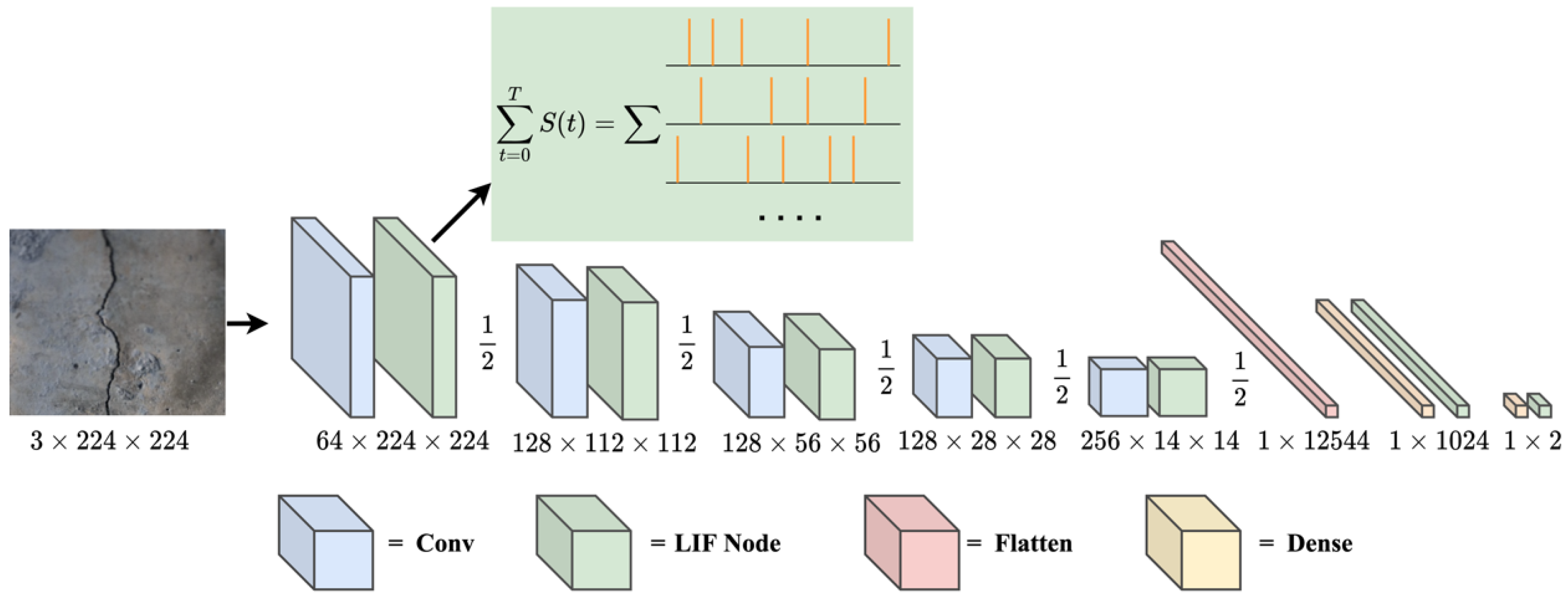
2.1. Network Structure of DCSNN
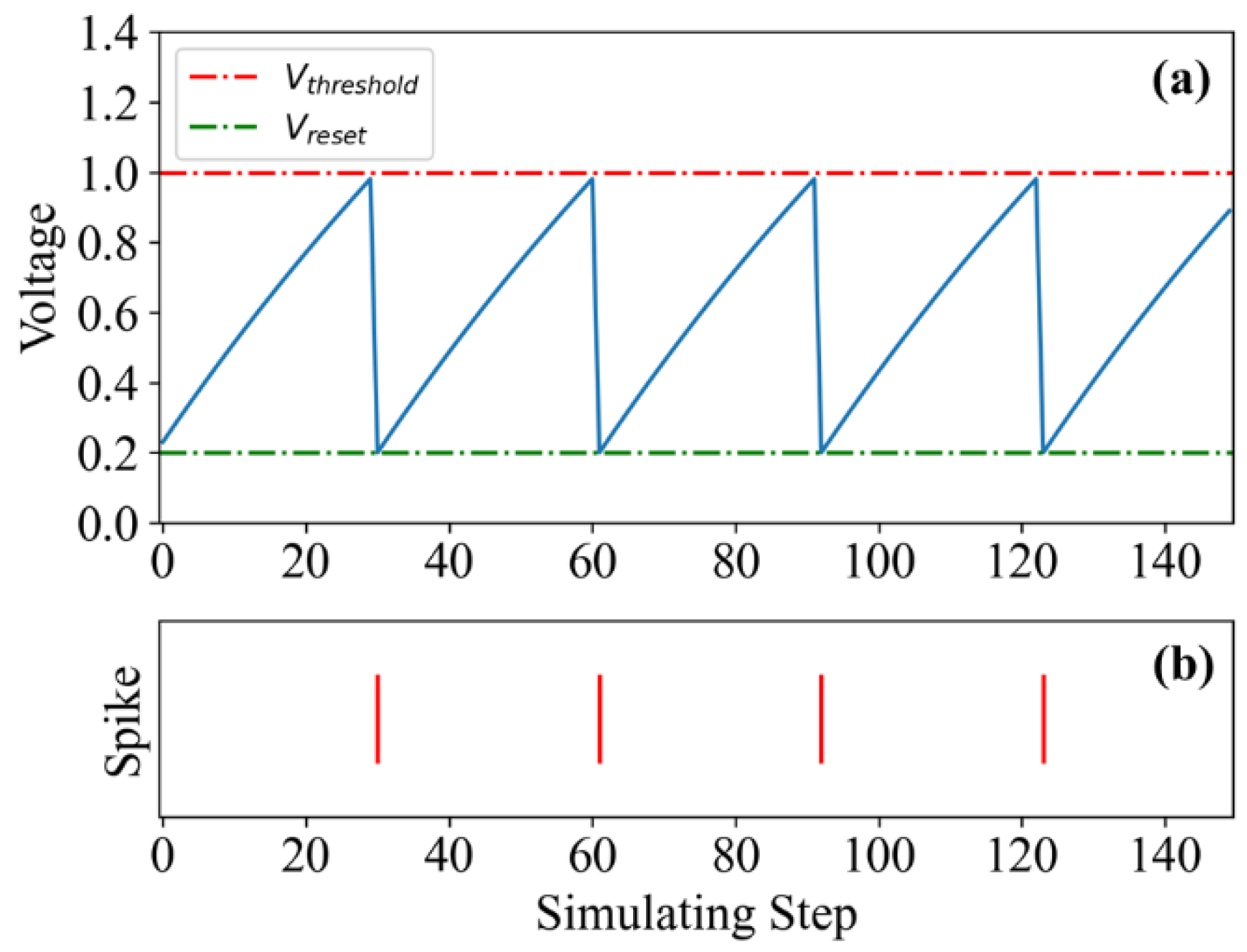
2.2. LIF Model
3. Training Algorithm
4. Experiments
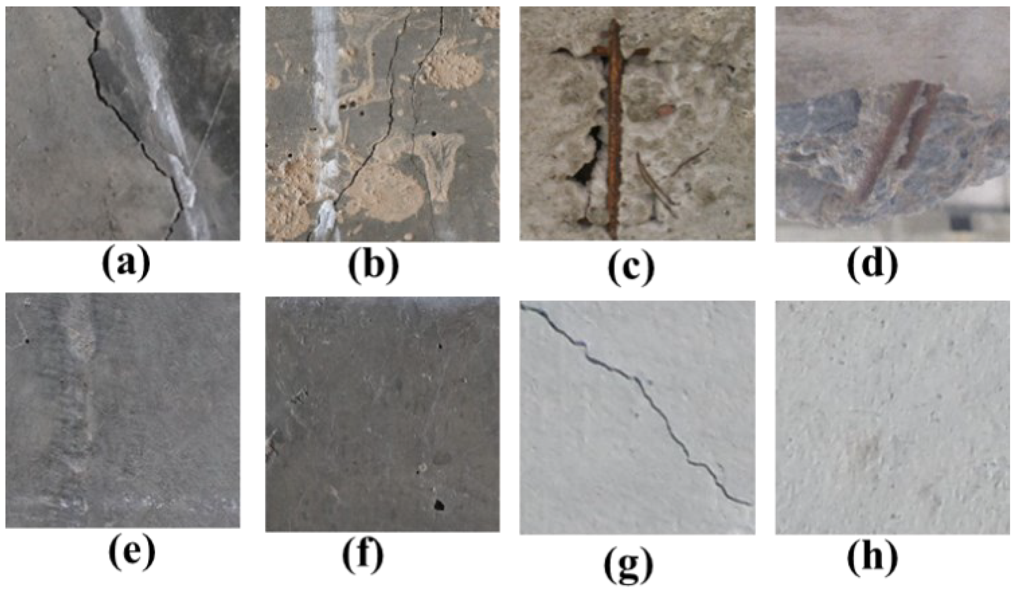
4.1. Datasets
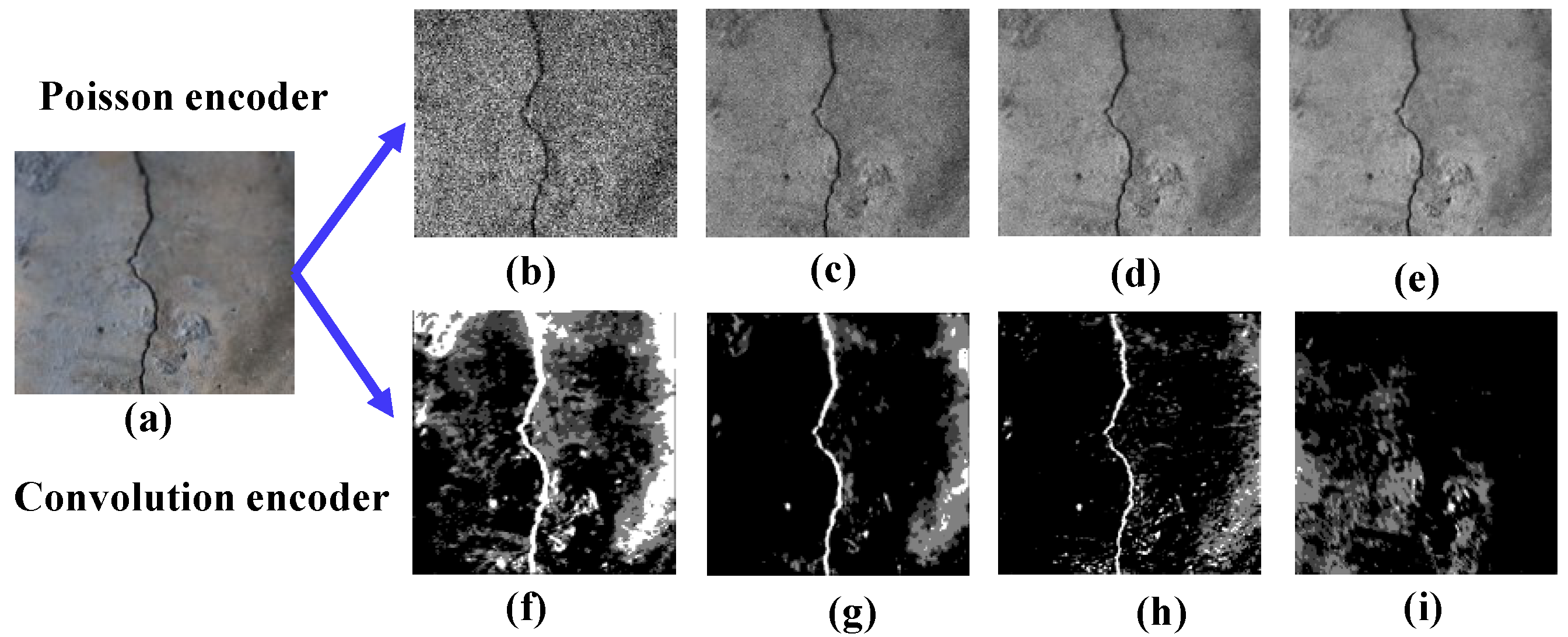
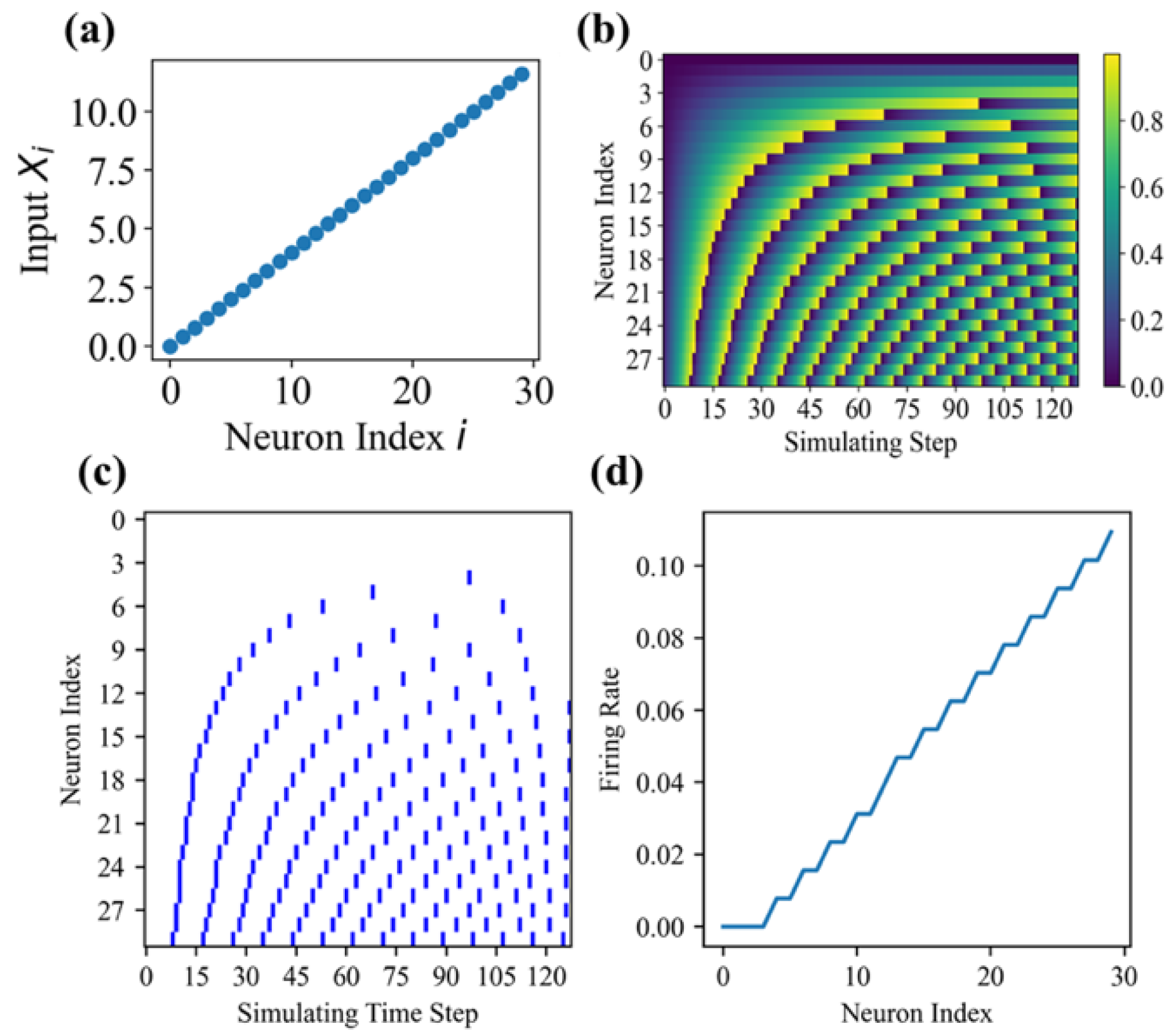
4.2. Spike Encoding Strategy
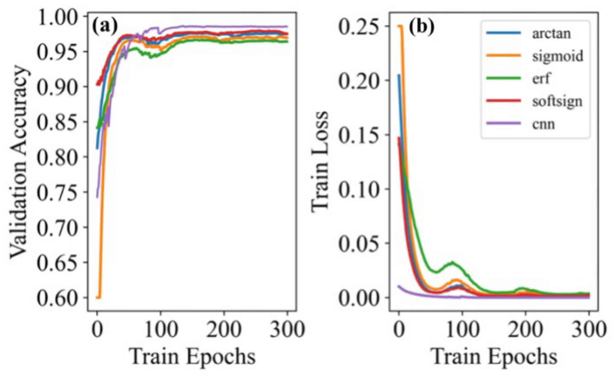
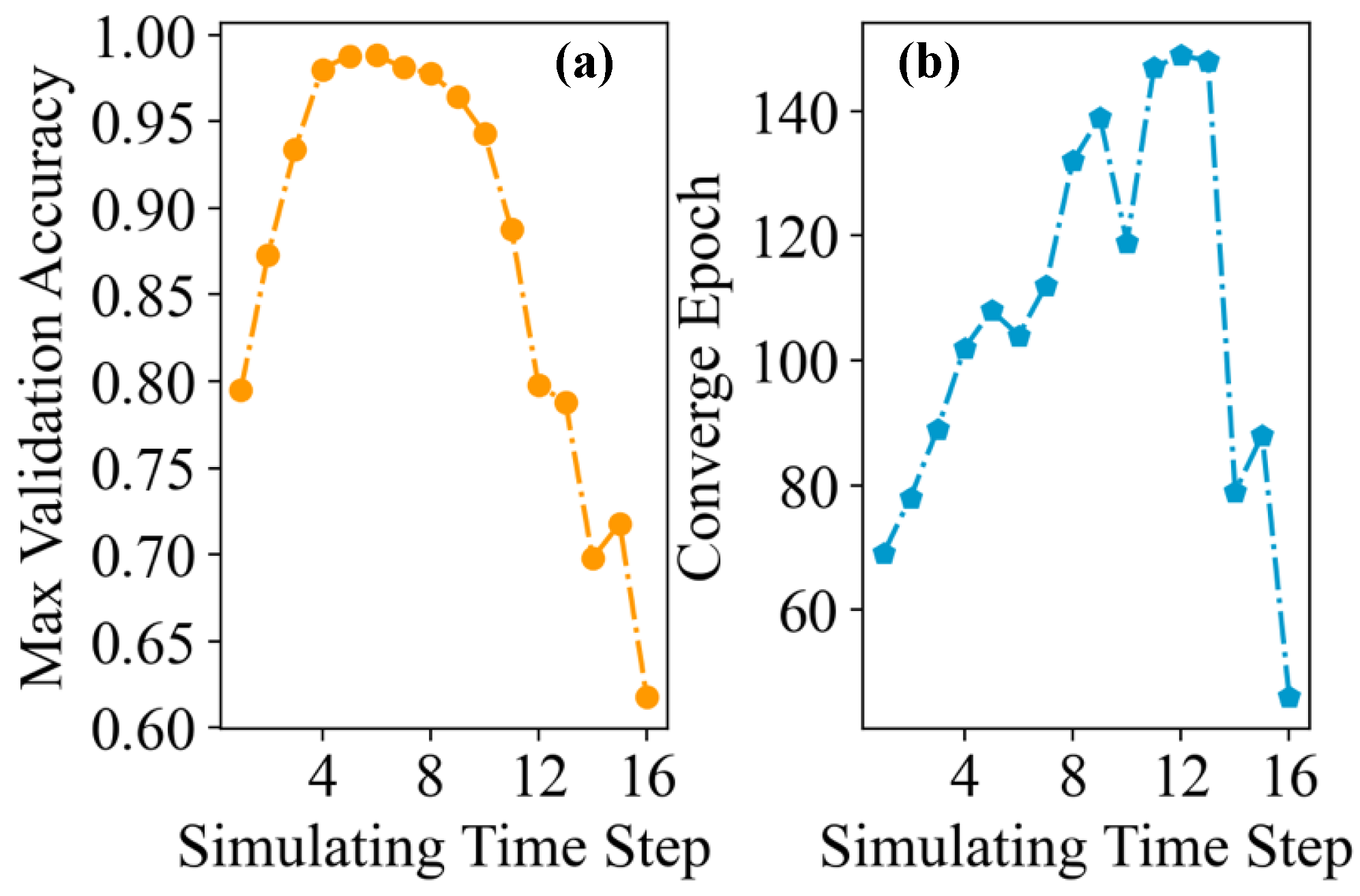
4.3. Training
4.4. Testing
4.5. Complexity Analysis
4.6. Hardware Implmentations
5. Conclusions
Author Contributions
Funding
Data Availability Statement
Conflicts of Interest
References
- Maass, W. Networks of spiking neurons: The third generation of neural network models. Neural Netw. 1997, 10, 1659–1671. [Google Scholar] [CrossRef]
- Wang, X.; Lin, X.; Dang, X. Supervised learning in spiking neural networks: A review of algorithms and evaluations. Neural Netw. 2020, 125, 258–280. [Google Scholar] [CrossRef] [PubMed]
- Taherkhani, A.; Belatreche, A.; Li, Y.; Cosma, G.; Maguire, L.; McGinnity, T. A review of learning in biologically plausible spiking neural networks. Neural Netw. 2020, 122, 253–272. [Google Scholar] [CrossRef] [PubMed]
- Caporale, N.; Dan, Y. Spike timing—Dependent plasticity: A Hebbian learning rule. Annu. Rev. Neurosci. 2008, 31, 25–46. [Google Scholar] [CrossRef] [Green Version]
- Diehl, P.; Cook, M. Unsupervised learning of digit recognition using spike-timing-dependent plasticity. Front. Comput. Neurosci. 2015, 9, 99. [Google Scholar] [CrossRef] [Green Version]
- Xiang, S.; Zhang, Y.; Gong, J. STDP-based unsupervised spike pattern learning in a photonic spiking neural network with VCSELs and VCSOAs. IEEE J. Sel. Top. Quantum Electron. 2019, 25, 1–9. [Google Scholar] [CrossRef]
- Xiang, S.; Ren, Z.; Song, Z. Computing primitive of fully VCSEL-based all-optical spiking neural network for supervised learning and pattern classification. IEEE Trans. Neural Netw. Learn. Syst. 2020, 32, 2494–2505. [Google Scholar] [CrossRef] [PubMed]
- Song, Z.; Xiang, S.; Cao, X.; Zhao, S.; Hao, Y. Experimental demonstration of photonic spike-timing dependent plasticity based on a VCSOA. Sci. China Inf. Sci. 2022, 65, 182401. [Google Scholar]
- Kheradpisheh, S.; Ganjtabesh, M.; Thorpe, S. STDP-based spiking deep convolutional neural networks for object recognition. Neural Netw. 2018, 99, 56–67. [Google Scholar] [CrossRef] [Green Version]
- Bohte, S.; Kok, J.; La Poutre, H. Error-backpropagation in temporally encoded networks of spiking neurons. Neurocomputing 2002, 48, 17–37. [Google Scholar] [CrossRef] [Green Version]
- Gütig, R.; Sompolinsky, H. The tempotron: A neuron that learns spike timing—Based decisions. Nat. Neurosci. 2006, 9, 420–428. [Google Scholar] [CrossRef] [PubMed]
- Ponulak, F.; Kasi’nski, A. Supervised learning in spiking neural networks with ReSuMe: Sequence learning, classification, and spike shifting. Neural Comput. 2010, 22, 467–510. [Google Scholar] [CrossRef] [PubMed]
- Wade, J.; McDaid, L.; Santos, J.; Sayers, H. SWAT: A spiking neural network training algorithm for classification problems. IEEE Trans. Neural Netw. 2010, 21, 1817–1830. [Google Scholar] [CrossRef] [PubMed] [Green Version]
- Florian, R. The chronotron: A neuron that learns to fire temporally precise spike patterns. PLoS ONE 2012, 7, e40233. [Google Scholar] [CrossRef] [Green Version]
- Mohemmed, A.; Schliebs, S.; Matsuda, S.; Kasabov, N. SPAN: Spike pattern association neuron for learning spatio-temporal spike patterns. Int. J. Neural Syst. 2012, 22, 1250012. [Google Scholar] [CrossRef] [PubMed]
- Eliasmith, C.; Anderson, C. Neural Engineering: Computation, Representation, and Dynamics in Neurobiological Systems; MIT press: Cambridge, MA, USA, 2003. [Google Scholar]
- Tsur, E. Neuromorphic Engineering: The Scientist’s, Algorithm Designer’s, and Computer Architect’s Perspectives on Brain-Inspired Computing; CRC Press: Boca Raton, FL, USA, 2021. [Google Scholar]
- Sporea, I.; Grüning, A. Supervised learning in multilayer spiking neural networks. Neural Comput. 2013, 25, 473–509. [Google Scholar] [CrossRef] [Green Version]
- Cao, Y.; Chen, Y.; Khosla, D. Spiking deep convolutional neural networks for energy-efficient object recognition. Int. J. Comput. Vis. 2015, 113, 54–66. [Google Scholar] [CrossRef]
- Lee, J.; Delbruck, T.; Pfeiffer, M. Training deep spiking neural networks using backpropagation. Front. Comput. Neurosci. 2016, 10, 508. [Google Scholar] [CrossRef] [Green Version]
- Lin, X.; Wang, X.; Hao, Z. Supervised learning in multilayer spiking neural networks with inner products of spike trains. Neurocomputing 2017, 237, 59–70. [Google Scholar] [CrossRef]
- Yamazaki, K.; Vo-Ho, V.-K.; Bulsara, D.; Le, N. Spiking neural networks and their applications: A Review. Brain Sci. 2022, 12, 863. [Google Scholar] [CrossRef]
- Taherkhani, A.; Belatreche, A.; Li, Y.; Maguire, L. A supervised learning algorithm for learning precise timing of multiple spikes in multilayer spiking neural networks. IEEE Trans. Neural Netw. Learn. Syst. 2018, 29, 5394–5407. [Google Scholar] [CrossRef] [PubMed] [Green Version]
- Kim, S.; Park, S.; Na, B.; Yoon, S. Spiking-YOLO: Spiking neural network for energy-efficient object detection. In Proceedings of the AAAI Conference on Artificial Intelligence, New York, NY, USA, 7–12 February 2020. [Google Scholar]
- Neftci, E.; Mostafa, H.; Zenke, F. Surrogate gradient learning in spiking neural networks: Bringing the power of gradient-based optimization to spiking neural networks. IEEE Signal Process. Mag. 2019, 36, 51–63. [Google Scholar] [CrossRef]
- Qiao, G.; Ning, N.; Zuo, Y.; Hu, S.; Yu, Q.; Liu, Y. Direct training of hardware-friendly weight binarized spiking neural network with surrogate gradient learning towards spatio-temporal event-based dynamic data recognition. Neurocomputing 2021, 457, 203–213. [Google Scholar] [CrossRef]
- Zenke, F.; Ganguli, S. SuperSpike: Supervised Learning in Multilayer Spiking Neural Networks. Neural Comput. 2018, 30, 1514–1541. [Google Scholar] [CrossRef]
- Shrestha, S.; Orchard, G. SLAYER: Spike Layer Error Reassignment in Time. In Proceedings of the Advances in Neural Information Processing Systems, Montréal, QC, Canada, 3–8 December 2018; pp. 1419–1428. [Google Scholar]
- Wu, Y.; Deng, L.; Li, G.; Zhu, J.; Xie, Y.; Shi, L. Direct training for spiking neural networks: Faster, larger, better. In Proceedings of the AAAI Conference on Artificial Intelligence, Hawaii, NA, USA, 27 January–1 February 2019; Volume 33, pp. 1311–1318. [Google Scholar]
- Wu, J.; Chua, Y.; Zhang, M.; Li, G.; Li, H.; Tan, K. A Tandem Learning Rule for Effective Training and Rapid Inference of Deep Spiking Neural Networks. arXiv 2020, arXiv:1907.01167. [Google Scholar] [CrossRef]
- Deng, L. Rethinking the performance comparison between SNNS and ANNS. Neural Netw. 2020, 121, 294–307. [Google Scholar] [CrossRef]
- Cha, Y.; Choi, W.; Büyüköztürk, O. Deep learning-based crack damage detection using convolutional neural networks. Comput.-Aided Civ. Infrastruct. Eng. 2017, 32, 361–378. [Google Scholar] [CrossRef]
- Chen, F.; Jahanshahi, M. NB-CNN: Deep learning-based crack detection using convolutional neural network and Naïve Bayes data fusion. IEEE Trans. Ind. Electron. 2017, 65, 4392–4400. [Google Scholar] [CrossRef]
- Dung, C. Autonomous concrete crack detection using deep fully convolutional neural network. Autom. Constr. 2019, 99, 52–58. [Google Scholar] [CrossRef]
- Deng, J.; Lu, Y.; Lee, V. Concrete crack detection with handwriting script interferences using faster region-based convolutional neural network. Comput.-Aided Civ. Infrastruct. Eng. 2020, 35, 373–388. [Google Scholar] [CrossRef]
- Yu, L.; He, S.; Liu, X. Engineering-oriented bridge multiple-damage detection with damage integrity using modified faster region-based convolutional neural network. Multimed. Tools Appl. 2022, 81, 18279–18304. [Google Scholar] [CrossRef]
- Yu, L.; He, S.; Liu, X. Intelligent crack detection and quantification in the concrete bridge: A deep learning-assisted image processing approach. Adv. Civ. Eng. 2022, 2022, 1813821. [Google Scholar] [CrossRef]
- Sengupta, A.; Ye, Y.; Wang, R.; Liu, C.; Roy, K. Going Deeper in Spiking Neural Networks: VGG and Residual Architectures. Front. Neurosci. 2019, 13, 95. [Google Scholar] [CrossRef] [PubMed]
- Wu, Y.; Deng, L.; Li, G.; Zhu, J.; Shi, L. Spatio-temporal backpropagation for training high-performance spiking neural networks. Front. Neurosci. 2018, 12, 331. [Google Scholar] [CrossRef]
- Yin, S.; Venkataramanaiah, S.; Chen, G.; Krishnamurthy, R.; Cao, Y.; Chakrabarti, C.; Seo, J. Algorithm and hardware design of discrete-time spiking neural networks based on back propagation with binary activations. In Proceedings of the 2017 IEEE Biomedical Circuits and Systems Conference (BioCAS), Torino, Italy, 19–21 October 2017. [Google Scholar]
- Dorafshan, S.; Thomas, R.; Maguire, M. SDNET2018: An annotated image dataset for non-contact concrete crack detection using deep convolutional neural networks. Data Brief 2018, 21, 1664–1668. [Google Scholar] [CrossRef]
- Github. Available online: https://github.com/fangwei123456/spikingjelly (accessed on 17 December 2019).
- Kingma, D.; Ba, J. Adam: A Method for Stochastic Optimization. Available online: https://arxiv.org/abs/1412.6980/ (accessed on 12 December 2014).
- He, K.; Sun, J. Convolutional neural networks at constrained time cost. In Proceedings of the IEEE Conference on Computer Vision and Pattern Recognition, Santiago, Chile, 7–13 December 2015; pp. 5353–5360. [Google Scholar]
- Davies, M.; Narayan, S.; Tsung-Han, L. Loihi: A neuromorphic manycore processor with on-chip learning. IEEE Micro 2018, 38, 82–99. [Google Scholar] [CrossRef]
- Hazan, A.; Ezra, E. Neuromorphic Neural Engineering Framework-Inspired Online Continuous Learning with Analog Circuitry. Appl. Sci. 2022, 12, 4528. [Google Scholar] [CrossRef]
- Kornijcuk, V.; Lim, H.; Seok, J. Leaky integrate-and-fire neuron circuit based on floating-gate integrator. Front. Neuro-Sci. 2016, 10, 212. [Google Scholar] [CrossRef]


| Layer (Type) | Output Shape | Parameter Number |
|---|---|---|
| Conv2d | [batch, 64, 224, 224] | 1728 |
| LIF Node | [T, batch, 64, 224, 224] | 0 |
| MaxPool2d | [batch, 128, 112, 112] | 0 |
| Conv2d | [batch, 128, 112, 112] | 73,728 |
| LIF Node | [T, batch, 128, 112, 112] | 0 |
| MaxPool2d | [batch, 128, 56, 56] | 0 |
| Conv2d | [batch, 128, 56, 56] | 147,456 |
| LIF Node | [T, batch, 128, 56, 56] | 0 |
| MaxPool2d | [batch, 128, 28, 28] | 0 |
| Conv2d | [batch, 256, 28, 28] | 147,456 |
| LIF Node | [T, batch, 256, 28, 28] | 0 |
| MaxPool2d | [batch, 256, 14, 14] | 0 |
| Conv2d | [batch, 256, 14, 14] | 294,912 |
| LIF Node | [T, batch, 256, 14, 14] | 0 |
| MaxPool2d | [batch, 256, 7, 7] | 0 |
| Flatten | [batch, 12544] | 0 |
| Linear | [batch, 1024] | 12,845,056 |
| LIF Node | [T, batch, 1024] | 0 |
| Linear | [batch, 2] | 2048 |
| LIF Node | [T, batch, 2] | 0 |
| Model | Accuracy on (%) | |
|---|---|---|
| Ours | SDNET2018 | |
| VGG7 | 98.67 | 84.79 |
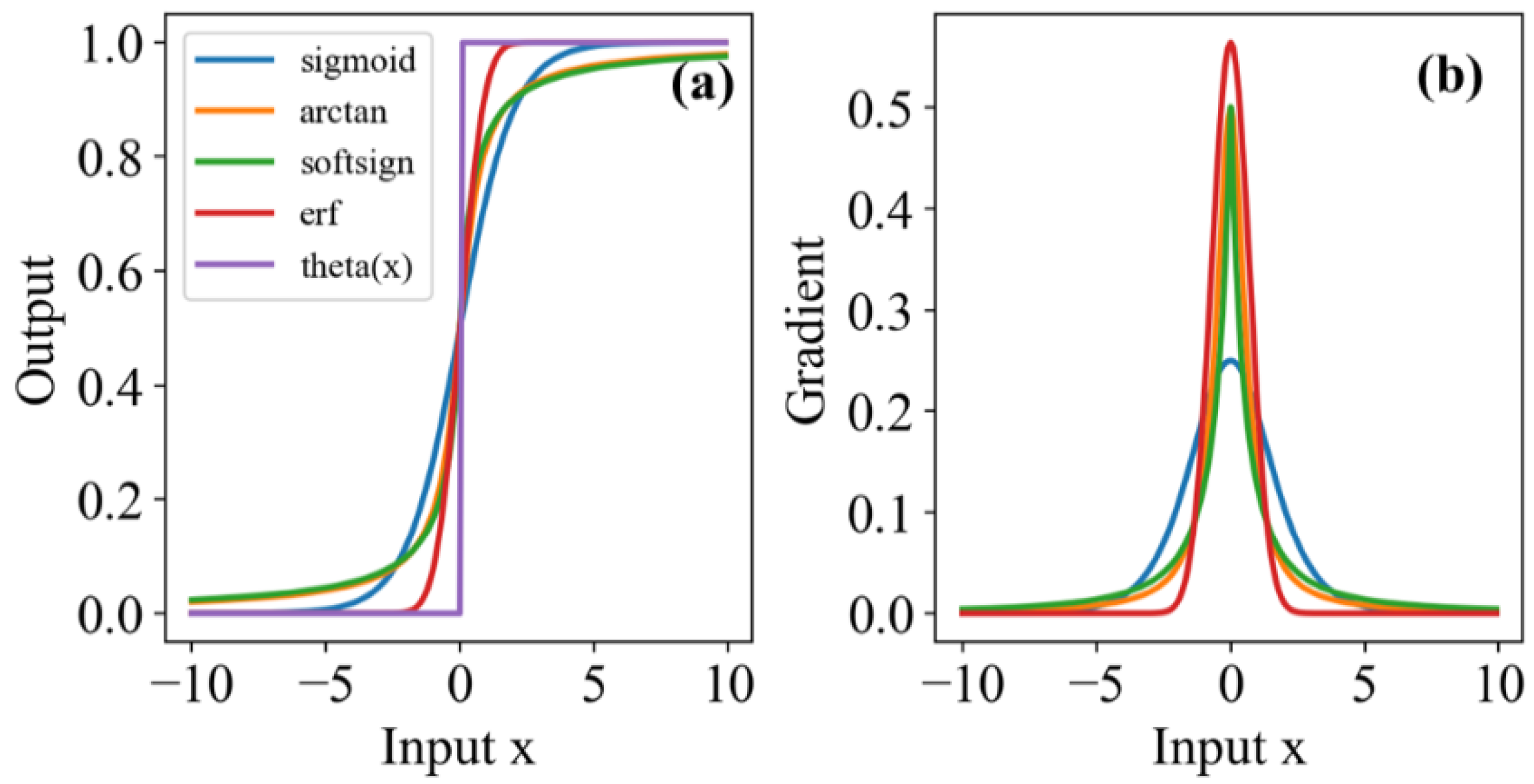
| Spiking VGG7T = 6 + softsign + Convolutional Encode | 97.83 | 78.45 |
| Spiking VGG7T = 6 + softsign + Poisson Encode | 91.22 | 70.47 |
| Spiking VGG7T = 6 + sigmoid + Convolutional Encode | 97.11 | 76.07 |
| Spiking VGG7T = 6 + erf + Convolutional Encode | 96.33 | 74.34 |
| Spiking VGG7T = 6 + arctan + Convolutional Encode | 97.67 | 76.68 |
| SDNN | 73.2 | 55.30 |
Publisher’s Note: MDPI stays neutral with regard to jurisdictional claims in published maps and institutional affiliations. |
© 2022 by the authors. Licensee MDPI, Basel, Switzerland. This article is an open access article distributed under the terms and conditions of the Creative Commons Attribution (CC BY) license (https://creativecommons.org/licenses/by/4.0/).
Share and Cite
Xiang, S.; Jiang, S.; Liu, X.; Zhang, T.; Yu, L. Spiking VGG7: Deep Convolutional Spiking Neural Network with Direct Training for Object Recognition. Electronics 2022, 11, 2097. https://doi.org/10.3390/electronics11132097
Xiang S, Jiang S, Liu X, Zhang T, Yu L. Spiking VGG7: Deep Convolutional Spiking Neural Network with Direct Training for Object Recognition. Electronics. 2022; 11(13):2097. https://doi.org/10.3390/electronics11132097
Chicago/Turabian StyleXiang, Shuiying, Shuqing Jiang, Xiaosong Liu, Tao Zhang, and Licun Yu. 2022. "Spiking VGG7: Deep Convolutional Spiking Neural Network with Direct Training for Object Recognition" Electronics 11, no. 13: 2097. https://doi.org/10.3390/electronics11132097
APA StyleXiang, S., Jiang, S., Liu, X., Zhang, T., & Yu, L. (2022). Spiking VGG7: Deep Convolutional Spiking Neural Network with Direct Training for Object Recognition. Electronics, 11(13), 2097. https://doi.org/10.3390/electronics11132097