Forward-Looking Imaging Based on the Linear Wavefront of the Modulated Field

Abstract

The vortex electromagnetic wave improves the range-azimuth forward-looking imaging performance with its spiral spatial phase distribution. However, the beam of the vortex electromagnetic wave is divergent, which makes it difficult to detect the targets near the center of the beam. In addition, the vortex electromagnetic wave only has the phase change in the azimuth direction and can hardly estimate the elevation position of the targets. In this paper, a linear wavefront control method based on the amplitude weighting of the array antenna is proposed. The modulated field has a phase gradient in both azimuth and elevation directions and has a maximum radiation intensity in the center of the beam. The imaging model based on the modulated field is theoretically derived and simulations are conducted to demonstrate the imaging performance. The modulated field constructed by the linear array can realize range-azimuth two-dimensional imaging with azimuth resolution of 1/5 beam width. The modulated field constructed by the circular array can realize range-azimuth-elevation three-dimensional imaging, and the resolution of the azimuth and elevation directions is 1/3 of the beam width.

1. Introduction

Orbital angular momentum (OAM) provides new degrees of freedom due to its particular physical property in optics [1] and microwaves [2]. With the characteristics of the spiral wavefront and the orthogonality brought by different topological charges, the vortex electromagnetic wave carrying OAM brings many advantages in wireless communication [3,4], rotational target detection [5,6,7], and radar imaging [8,9,10]. Forward-looking radar imaging usually refers to two dimensions. One is the range dimension, and the other one is the orthogonal azimuth dimension. Electromagnetic vortex imaging has great potential to achieve high azimuth resolution, and could distinguish targets that are very close in azimuth dimension, especially under the relatively stationary condition [11,12,13].

In 2015, Fourier transform method was first introduced for two-dimensional electromagnetic vortex imaging [14]. The echo models of the multiple-in–multiple-out mode and multiple-in–single-out mode were established. The range resolution of electromagnetic vortex imaging depends on the bandwidth of the transmitted signal, and the azimuth resolution depends on the number of the OAM modes. In the follow-up studies, pattern-optimization methods were proposed to enhance the imaging performance [15]. The main lobe direction could be optimized by the concentric uniform circular array to ensure that the vortex electromagnetic waves with different modes could illuminate the targets simultaneously [16,17]. By collimating the main lobe direction and suppressing the side lobe level, the echo energy is enhanced, and vortex imaging is more resistant to noise [18]. Besides the Fourier transform method, other algorithms, such as power spectrum density (PSD) estimation [19] and multiple signal classification (MUSIC) [20], were also applied to improve the azimuth resolution of electromagnetic vortex imaging. By establishing an autoregressive model of the signal, the PSD method could obtain sharp spectral peaks. The MUSIC method estimates the peak position according to the orthogonality of the signal subspace and the noise subspace. Both the PSD and MUSIC methods improved azimuth resolution from the perspective of super-resolution signal processing. To reduce the number of OAM modes used during electromagnetic vortex imaging, sparse Bayesian learning (SBL) is introduced to reconstruct the image [21,22]. By establishing the imaging equation, the radar cross section (RCS) of targets at different positions are estimated. Moreover, based on the SBL framework, the enhanced SBL and variational sparse Bayesian inference are utilized to achieve higher azimuth resolution. The vortex electromagnetic wave has significantly improved the forward-looking imaging performance, but there are still some disadvantages in application [23,24]. The spiral spatial phase of the vortex beam leads to the phase singularity in the middle, so the radiation pattern of the vortex beam is doughnut-shaped. The targets near the center of the beam are difficult to detect. In addition, the vortex imaging method requires multiple modes of vortex electromagnetic waves to illuminate the targets simultaneously. But the property of the Bessel function determines that the main lobe direction of the vortex beam with different OAM modes are inconsistent. The vortex electromagnetic wave only has the spiral phase front in the azimuth direction and can hardly estimate the elevation positions of the targets.

To avoid the beam divergence of the vortex beam, we proposed an effective forward-looking imaging method by constructing the modulated field with a linear wavefront. By adjusting the amplitude weighting coefficient of the antenna array units, the modulated field has linear phase distribution in azimuth and elevation directions. In Section 2, the two-dimensional and three-dimensional imaging methods are proposed. The amplitude and phase distribution of the modulated field are analysed first, and the computational imaging method based on the linear wavefront are derived subsequently. In Section 3, the numerical simulations of different imaging scenarios are carried out to demonstrate the effectiveness of the proposed method. An advantage of the proposed method is that the maximum radiation intensity is at the center of the beam. There is no blind area at the center and no beam collimation is required, which is more suitable for radar forward-looking imaging applications. Moreover, the modulated field has phase changes in azimuth and elevation dimensions simultaneously. The targets at different elevation positions could be distinguished and imaged.

2. Method

2.1. Two-Dimensional Imaging Based on a Linear Array

The phase of the modulated field constructed by a linear array changes linearly along the azimuth direction. This characteristic could be used to distinguish targets with different azimuth positions at the same range. Combined with the range resolution brought by the bandwidth of the transmitted signal, the range-azimuth forward-looking imaging could be achieved. The linear array with N units is located on the XOY plane as shown in Figure 1. The linear wavefront could be generated by the unequal amplitude weighting of the array units. In a real radar system, the amplitude control of the array units is usually realized by adjustable amplifiers or attenuators. As the number of units increases, the complexity and the cost of the radar system will significantly increase. Considering the complexity of the system and the generation of the linear wavefront, we chose a compromised value of $N=8$. The center frequency of the antenna is $f_c=17$ GHz. The wavelength is $\lambda =c/f_c$, where c is the speed of light. The length of the array antenna is a. The large antenna length will lead to the high level of side lobe and grating lobe. The small antenna length will lead to the little adjustable range of the phase gradient. Thus, the array is designed as length $a=7.5\lambda$, and N = 8 units are non-uniformly arranged. The intervals of the eight units are $4\Delta$, $3\Delta$, $2\Delta$, $2\Delta$, $2\Delta$, $3\Delta$, $4\Delta$ ($\Delta =a/20$), respectively. The projection of point $P(r,\theta ,\phi )$ on the XOZ plane is $P^{\prime }$, and the azimuth angle $\alpha$ is defined as the angle between $O{P}^{\prime }$ and Z-axis.

To generate the modulated field, we use the same phase but different amplitude signals to feed each unit. The electric pattern F of the linear array could be expressed as [25].

$$F=\sum _{n=1}^N{I}_{n}exp\left(i\mathit{k}{\mathit{r}}_{\mathit{n}}\right)=\sum _{n=1}^N{I}_{n}exp\left[ik(x_{n}sin\theta cos\phi )\right],$$

(1)

where the wave number vector is $\mathit{k}=ksin\theta cos\phi \widehat{\mathit{x}}+ksin\theta sin\phi \widehat{\mathit{y}}+kcos\theta \widehat{\mathit{z}}$, $k=2\pi /\lambda$. $I_n$ and $x_n$ are the amplitude coefficient and X-axis coordinate of the n-th unit, respectively. Therefore, the phase pattern of F is

$$P=\mathbf{angle}\left(F\right)=arctan\frac{\mathbf{imag}\left(F\right)}{\mathbf{real}\left(F\right)}=arctan\frac{{\sum }_{n=1}^N{I}_{n}sin[k(x_{n}sin\theta cos\phi ]}{{\sum }_{n=1}^I{I}_{n}cos\left[k(x_{n}sin\theta cos\phi )\right]}.$$

(2)

When $\theta$ is close to 0, the phase gradient along $\phi$ is

$$\begin{array}{cc}\hfill \frac{\partial P}{\partial \theta }{|}_{\theta =0}& \approx arctan\frac{{\sum }_{n=1}^N{I}_{n}k(x_{n}cos\phi )}{{\sum }_{n=1}^N{I}_n}\hfill \\ \hfill & \approx k\frac{{\sum }_{n=1}^N{I}_n{x}_n}{{\sum }_{n=1}^N{I}_n}cos\phi \hfill \\ \hfill & =k{O}_{x}cos\phi ,\hfill \end{array}$$

(3)

where $O_x=\frac{{\sum }_{n=1}^N{I}_n{x}_n}{{\sum }_{n=1}^N{I}_n}$ is the equivalent phase center of the antenna array. When $\phi =0$, we have the phase gradient $L=k{O}_x$ along azimuth direction.

Figure 2 shows the simulation results of the modulated field with phase gradient $L=0,3,6,9$. The amplitude coefficients are shown in

Table 1. Relative amplitude coefficients of eight units.

Field	1	2	3	4	5	6	7	8	L	${\mathit{\theta }}_{\mathit{bw}}$
I	1.00	1.00	1.00	1.00	1.00	1.00	1.00	1.00	0	${6.4}^{\circ }$
II	1.41	1.17	1.08	1.01	0.94	0.88	0.81	0.66	3	${6.4}^{\circ }$
III	1.64	1.40	1.23	1.08	0.92	0.77	0.60	0.32	6	${7.2}^{\circ }$
IV	2.08	1.68	1.34	1.06	0.80	0.55	0.34	0.11	9	${8.2}^{\circ }$

. Figure 2a,b is the amplitude pattern and the phase distributions along azimuth direction (XOZ plane). Figure 2c shows the two-dimensional phase distribution within the main lobe. When the amplitude coefficients of all array units are equal, the wavefront has the property of the plane wave. When the modulated field is constructed, the phase changes linearly along the azimuth direction. The phase along the elevation direction is almost unchanged. The phase gradient L is controlled by the amplitude coefficient. As the gradient L increases, the phase changes more rapidly, and the main lobe width ${\theta }_{bw}$ is slightly broadened. Although the gradient $L=3,6,9$, the phase variation range is approximatively ±15${}^{\circ }$, ±30${}^{\circ }$, ±45${}^{\circ }$ within the beam range of ±5${}^{\circ }$. Echoes of targets at different azimuth positions are easier to distinguish with a larger gradient.

Under the illumination of the modulated field, the echo phases of the scattering points at different azimuth positions are different. According to the spatial phase distribution of the modulated field, an equation is established to estimate the RCS of the scattering points to achieve range-azimuth forward-looking imaging. The linear frequency modulation (LFM) signal transmitted by the n-th unit is

$$s_{tn}\left(t\right)=I_n·rect(t/T)·exp\left(i\pi K{t}^2\right)·exp\left(i2\pi f_{c}t\right),$$

(4)

where T is the pulse width and K is the frequency modulation slope of the LFM signal. The RCS of the scattering point $P\left(r,\theta ,\phi \right)$ in the far field is $\sigma$. After the transmitted signal is reflected by P, the n-th unit receives the echo with the same amplitude coefficient $I_n$. The received signal of the n-th unit is

$$\begin{array}{cc}\hfill s_{rn}\left(t\right)=& \sigma ·I_n^2·rect\left(\frac{t-2t_n}{T}\right)·exp\left[i\pi K{\left(t-2t_n\right)}^2\right]\hfill \\ & ·exp\left[i2\pi f_c\left(t-2t_n\right)\right],\hfill \end{array}$$

(5)

where $t_n$ is the time delay from the n-th unit to point P. $t_n=t^{\prime }-\Delta d/c$, $t^{\prime }=r/c$ and $\Delta d=x_{n}sin\theta cos\phi$. In most radar applications, the target range is much larger than the array size; therefore $t^{\prime }\gg \Delta d/c$. In the amplitude approximation, $rect\left[\left(t-2t_n\right)/T\right]\approx rect\left[\left(t-2t^{\prime }\right)/T\right]$. And in the phase approximation, the quadratic term for $\Delta d/c$ could be ignored. Equation (5) could be approximated as

$$\begin{array}{cc}\hfill s_{rn}\left(t\right)\approx & \sigma I_n^2·rect\left(\frac{t-2t^{\prime }}{T}\right)·exp\left[i\pi K{\left(t-2t^{\prime }+2\Delta d/c\right)}^2\right]\hfill \\ \hfill & ·exp\left[i2\pi f_c\left(t-2t^{\prime }+2\Delta d/c\right)\right]\hfill \\ \hfill =& \sigma I_n^2·rect\left(\frac{t-2t^{\prime }}{T}\right)·exp\left[i\pi K{\left(t-2t^{\prime }\right)}^2\right]·exp\left[i2\pi f_c\left(t-2t^{\prime }\right)\right]\hfill \\ \hfill & ·exp\left\{i2\pi \left[K\left(t-2t^{\prime }\right)+f_c\right]2\Delta d/c\right\}.\hfill \end{array}$$

(6)

When the bandwidth of the LFM signal is much smaller than the carrier frequency, $2\pi \left[K\left(t-2t^{\prime }\right)+f_c\right]/c\approx 2\pi f_c/c=k$. The sum echo of all array units is

$$\begin{array}{cc}\hfill s_r\left(t\right)=& \sigma ·rect\left(\frac{t-2t^{\prime }}{T}\right)·exp\left[i\pi K{\left(t-2t^{\prime }\right)}^2\right]·exp\left[i2\pi f_c\left(t-2t^{\prime }\right)\right]\hfill \\ \hfill & \underset{n=1}{\stackrel{N}{·\sum }}{I}_n^2·exp\left[i2k{x}_{n}sin\theta cos\phi \right].\hfill \end{array}$$

(7)

According to the derivation of the phase distribution within the main lobe of the modulated field in Equation (1) to (3), ${\sum }_{n=1}^N{I}_n^{2}exp\left[i2k{x}_{n}sin\theta cos\phi \right]$ could be expressed as $exp\left(iL\alpha \right)$. $L=2k{\sum }_{n=1}^N{I}_n^2{x}_n/{\sum }_{n=1}^N{I}_n^2$ is the phase gradient in echo. Assuming that there are M scattering points at the same range r, the azimuth angle and the RCS of the m-th scattering point are ${\alpha }_m$ and ${\sigma }_m$. The total echo of M scattering points can be expressed as

$$\begin{array}{cc}\hfill s\left(t\right)=& rect\left[\frac{t-2r/c}{T}\right]exp\left[i\pi K{(t-2r/c)}^2\right]\hfill \\ \hfill & exp\left[i2\pi f_c\left(t-2r/c\right)\right]·\sum _{m=1}^M{\sigma }_{m}exp\left(iL{\alpha }_m\right).\hfill \end{array}$$

(8)

The echo after down-conversion and LFM signal pulse compression is

$$\begin{array}{cc}\hfill y\left(t\right)=& sinc\left[KT\left(t-2r/c\right)\right]exp\left(-i4\pi f_{c}r/c\right)·\sum _{m=1}^M{\sigma }_{m}exp(i·L{\alpha }_m)\hfill \\ \hfill =& A\left(t\right)·\sum _{m=1}^M{\sigma }_{m}exp\left(iL{\alpha }_m\right),\hfill \end{array}$$

(9)

where $A\left(t\right)$ is the term independent of the azimuth angle. The scattering points with different azimuth angle at the same range are still superimposed together, as shown in term ${\sum }_{m=1}^M{\sigma }_{m}exp\left(iL{\alpha }_m\right)$. The azimuth direction within the main lobe is divided into M discrete imaging grids, and D modulated fields with phase gradient $L_d$ are constructed. The echo of D modulated fields can be expressed in matrix form as

$$\mathbf{y}=\mathbf{Hx}+\mathbf{n}$$

$$\left[\begin{array}{c}{y}_1\left(t\right)\\ y_2\left(t\right)\\ ...\\ y_D\left(t\right)\end{array}\right]=A\left(t\right)\left[\begin{array}{c}exp\left(i{L}_1{\alpha }_1\right)\\ exp\left(i{L}_2{\alpha }_1\right)\\ ...\\ exp\left(i{L}_D{\alpha }_1\right)\end{array}\begin{array}{c}\\ \\ \\ \end{array}\begin{array}{c}exp\left(i{L}_1{\alpha }_2\right)\\ exp\left(i{L}_2{\alpha }_2\right)\\ ...\\ exp\left(i{L}_D{\alpha }_2\right)\end{array}\begin{array}{c}\\ \\ \\ \end{array}\begin{array}{c}...\\ ...\\ \\ ...\end{array}\begin{array}{c}\\ \\ \\ \end{array}\begin{array}{c}exp\left(i{L}_1{\alpha }_M\right)\\ exp\left(i{L}_2{\alpha }_M\right)\\ ...\\ exp\left(i{L}_D{\alpha }_M\right)\end{array}\right]·\left[\begin{array}{c}{\sigma }_1\\ {\sigma }_2\\ ...\\ {\sigma }_M\end{array}\right]+\left[\begin{array}{c}{n}_1\\ n_2\\ ...\\ n_D\end{array}\right].$$

(10)

In Equation (10), x is the unknown RCS vector of the scattering points at different azimuth position. H is the measurement matrix consisting of the D modulated fields. Each row in H represents the spatial phase distribution of the modulated field with the phase gradient $L_d$. y is the echo vector consisting of $y_d\left(t\right)$. n indicates the Gaussian noise. When $D\ge M$ and H is non-singular, the imaging equation would have a unique solution for x. Create an optimization objective function

$$\underset{\mathbf{x}}{\widehat{\mathbf{x}}=argmin}{∥\mathbf{y}-\mathbf{Hx}∥}_2^2.$$

(11)

After obtaining the optimal solution $\widehat{\mathbf{x}}$ from echo y and measurement matrix H, the RCS of the scattering points at different azimuth position could be estimated. The scattering points at different range are distinguished by LFM signal pulse compression. After pulse compression, the azimuth distribution at each range is reconstructed by Equations (10) and (11). Finally, the range-azimuth two-dimensional forward-looking image of the targets could be obtained.

2.2. Three-Dimensional Imaging Based on a Circular Array

The modulated field constructed by the linear array only has linear phase change along the azimuth direction. There is almost no difference in the echo phases of the targets at the same azimuth but different elevation positions. Therefore, the linear array has no imaging capability of elevation dimension. The modulated field constructed by a circular array has phase change along the azimuth and elevation directions, which could be used to distinguish the targets at different elevation positions. Assuming that the circular array is located on the XOY plane, as shown in Figure 3, and the center of the array is located at the coordinate origin O. The array radius is $a=\lambda$, and the number of array units is $N=8$. The coordinate of each array unit is $\left(x_n,y_n,0\right)$, $x_n=acos{\phi }_n$, $y_n=a\sin {\phi }_n$. Let the projection of point $P\left(r,\theta ,\phi \right)$ on the XOZ plane be $P^{\prime }$, and the projection on the YOZ plane be $P^{″}$. The azimuth angle $\alpha$ is defined as the angle between $O{P}^{\prime }$ and the Z-axis, and the elevation angle $\beta$ is defined as the angle between $O{P}^{″}$ and the Z-axis. Similar to the linear array, we use the same phase but different amplitude signals feed for each unit to generate the modulated field. The electric pattern of the circular array in the far field can be expressed as

$$F=\underset{n=1}{\sum ^N}{I}_{n}exp\left[-iksin\theta \left(x_{n}cos\phi +y_{n}sin\phi \right)\right].$$

(12)

When $\theta$ is close to 0, the phase gradient along $\phi$ is

$$\begin{array}{cc}\hfill \frac{\partial P}{\partial \theta }{|}_{\theta =0}=& arctan\frac{{\sum }_{n=1}^N{I}_{n}ksin\theta (x_{n}cos\phi +y_{n}sin\phi )}{{\sum }_{n=1}^I{I}_n}\hfill \\ \hfill =& k\frac{{\sum }_{n=1}^N{I}_n{x}_n}{{\sum }_{n=1}^N{I}_n}cos\phi +k\frac{{\sum }_{n=1}^N{I}_n{y}_n}{{\sum }_{n=1}^N{I}_n}sin\phi \hfill \\ \hfill =& k{O}_{x}cos\phi +k{O}_{y}sin\phi ,\hfill \end{array}$$

(13)

where $O_x=\frac{{\sum }_{n=1}^N{I}_n{x}_n}{{\sum }_{n=1}^N{I}_n}$ and $O_y=\frac{{\sum }_{n=1}^N{I}_n{y}_n}{{\sum }_{n=1}^N{I}_n}$ are the equivalent phase center in x and y directions. When $\phi =0$, we have the phase gradient $L_{\alpha }=k{O}_x$ along azimuth direction. When $\phi =\pi /2$, we have the phase gradient $L_{\beta }=k{O}_y$ along elevation direction. The phase gradient value is $L=\sqrt{L_{\alpha }^2+L_{\beta }^2}$ and the direction is ${\phi }_g=arctan(L_{\beta }/L_{\alpha })$.

Figure 4 shows the two-dimensional amplitude and phase distributions that are simulated by electromagnetic simulation software HFSS (High Frequency Structure Simulator, Ansoft). The gradient value is $L=2.5$, and the phase gradient directions are ${\phi }_g={37}^{\circ }$, ${86}^{\circ }$, ${211}^{\circ }$, ${285}^{\circ }$, respectively. The amplitude coefficients of antenna units are shown in

Table 2. Relative amplitude coefficients of the circular array units.

1	2	3	4	5	6	7	8	L	${\mathit{\phi }}_{\mathit{g}}$	${\mathit{L}}_{\mathit{\alpha }}$	${\mathit{L}}_{\mathit{\beta }}$
1.66	1.71	1.55	0.85	0.33	0.28	0.44	1.14	2.5	${37}^{\circ }$	2.03	1.53
1.07	1.64	1.71	1.58	0.92	0.35	0.28	0.41	2.5	${86}^{\circ }$	0.17	2.48
0.35	0.28	0.50	1.24	1.68	1.71	1.48	0.75	2.5	${211}^{\circ }$	−2.18	−1.31
1.26	0.51	0.28	0.31	0.73	1.48	1.71	1.68	2.5	${285}^{\circ }$	0.65	−2.41

. Figure 5 shows the amplitude and phase patterns in the azimuth direction (XOZ plane) and elevation direction (YOZ plane) of the modulated fields with ${\phi }_g={37}^{\circ }$, ${86}^{\circ }$, ${211}^{\circ }$, ${285}^{\circ }$. The modulated field constructed by the circular array has a linear phase change along the azimuth direction $\alpha$ and elevation direction $\beta$. The phase gradient value L and direction ${\phi }_g$ could be adjusted by the amplitude coefficients. Generated by the same circular array, the vortex electromagnetic wave with topological charge number $l=1$ has the opening angle ${17}^{\circ }$, as shown in Figure 6. The radiation intensity within $\pm 9^{\circ }$ of the beam center is weak. Compared to the vortex beam, the modulated field has the maximum radiation intensity at the center of the beam and the 3dB beam width is approximately $\pm {10}^{\circ }$. This characteristic avoids the divergence of the vortex beam and significantly improves the detection capability of the targets near the beam center.

The n-th array unit transmits the LFM signal with an amplitude coefficient $I_n$. When the array is circular, $\Delta d$ in the time delay $t_n$ from the n-th unit to point P becomes $x_{n}sin\theta cos\phi +y_{n}sin\theta sin\phi$. The n-th unit receives the echo with the same amplitude coefficient $I_n$. The echo of the circular array could be expressed as

$$\begin{array}{cc}\hfill s_r\left(t\right)=& \sigma ·rect\left(\frac{t-2t^{\prime }}{T}\right)·exp\left[i\pi K{\left(t-2t^{\prime }\right)}^2\right]·exp\left[i2\pi f_c\left(t-2t^{\prime }\right)\right]\hfill \\ \hfill & \underset{n=1}{\stackrel{N}{·\sum }}{I}_{n}exp\left[i2ksin\theta \left(x_{n}cos\phi +y_{n}sin\phi \right)\right].\hfill \end{array}$$

(14)

The term ${\sum }_{n=1}^N{I}_{n}exp\left[i2ksin\theta \left(x_{n}cos\phi +y_{n}sin\phi \right)\right]$ can be expressed as $exp\left[i\left(L_{\alpha }\alpha +L_{\beta }\beta \right)\right]$. $L_{\alpha }={2k\sum }_{n=1}^N{I}_n^2{x}_n/{\sum }_{n=1}^N{I}_n^2$ and $L_{\beta }={2k\sum }_{n=1}^N{I}_n^2{y}_n/{\sum }_{n=1}^N{I}_n^2$ are the phase gradients along the azimuth and elevation directions in the echo, respectively. Compared with the linear array, the echo of the circular array increases the term $exp\left(i{L}_{\beta }\beta \right)$ brought by the elevation position of the scattering point. Assuming that there are M scattering points at the same range r, the azimuth angle, elevation angle and RCS of the m-th scattering point are ${\alpha }_m$, ${\beta }_m$ and ${\sigma }_m$, respectively. The sum echo of the M scattering points is

$$\begin{array}{cc}\hfill s\left(t\right)=& rect\left[\frac{t-2r/c}{T}\right]exp\left[i2\pi f_c\left(t-2r/c\right)\right]·exp\left[i\pi K{(t-2r/c)}^2\right]\hfill \\ \hfill & \sum _m^M{\sigma }_{m}exp\left[i\left(L_{\alpha }{\alpha }_m+L_{\beta }{\beta }_m\right)\right].\hfill \end{array}$$

(15)

After down-conversion and LFM signal pulse compression, the echo is

$$\begin{array}{cc}\hfill y\left(t\right)=& sinc\left[KT\left(t-2r/c\right)\right]·exp\left(-i4\pi f_{c}r/c\right)\hfill \\ \hfill & ·\sum _m^M{\sigma }_{m}exp\left\{i\left(L_{\alpha }{\alpha }_m+L_{\beta }{\beta }_m\right)\right\}\hfill \\ \hfill =& A\left(t\right)·\sum _m^M{\sigma }_{m}exp\left\{i\left(L_{\alpha }{\alpha }_m+L_{\beta }{\beta }_m\right)\right\}.\hfill \end{array}$$

(16)

The scattering points with different azimuth and elevation positions at the same range are superimposed together. Assuming that the azimuth and elevation within the main lobe are divided into $K\times K=M$ discrete grids, D modulated fields with phase gradient value L and direction ${\phi }_{dg}$ are constructed for imaging. The phase gradient in the azimuth and elevation directions are $L_{d\alpha }$ and $L_{d\beta }$, respectively. The imaging equation could be established as

$$\mathbf{y}=\mathbf{Hx}+\mathbf{n},$$

(17)

$$\left[\begin{array}{c}{y}_1\left(t\right)\\ y_2\left(t\right)\\ ...\\ y_D\left(t\right)\end{array}\right]=A\left(t\right)\left[\begin{array}{c}exp\left[i\left(L_{1\alpha }{\alpha }_1+L_{1\beta }{\beta }_1\right)\right]\\ exp\left[i\left(L_{2\alpha }{\alpha }_1+L_{2\beta }{\beta }_1\right)\right]\\ ...\\ exp\left[i\left(L_{D\alpha }{\alpha }_1+L_{D\beta }{\beta }_1\right)\right]\end{array}\begin{array}{c}exp\left[i\left(L_{1\alpha }{\alpha }_2+L_{1\beta }{\beta }_1\right)\right]\\ exp\left[i\left(L_{2\alpha }{\alpha }_2+L_{2\beta }{\beta }_1\right)\right]\\ ...\\ exp\left[i\left(L_{D\alpha }{\alpha }_2+L_{D\beta }{\beta }_1\right)\right]\end{array}\begin{array}{c}...\\ ...\\ ...\\ ...\end{array}\begin{array}{c}exp\left[i\left(L_{1\alpha }{\alpha }_K+L_{1\beta }{\beta }_K\right)\right]\\ exp\left[i\left(L_{2\alpha }{\alpha }_K+L_{2\beta }{\beta }_K\right)\right]\\ ...\\ exp\left[i\left(L_{D\alpha }{\alpha }_K+L_{D\beta }{\beta }_K\right)\right]\end{array}\right]\left[\begin{array}{c}{\sigma }_{11}\\ {\sigma }_{21}\\ ...\\ {\sigma }_{KK}\end{array}\right]+\left[\begin{array}{c}{n}_1\\ n_2\\ ...\\ n_D\end{array}\right].$$

Each row in the measurement matrix H represents the spatial phase distribution of the modulated field constructed by the circular array. Creating the same optimization objective function as Equation (11) and estimating the RCS of each grid, the azimuth-elevation two-dimensional imaging could be achieved for scattering points at the same range. In summary, LFM pulse compression is performed firstly to distinguish targets at different range, and then the azimuth and elevation images are reconstructed for each range. The range-azimuth-elevation three-dimensional image could be finally obtained.

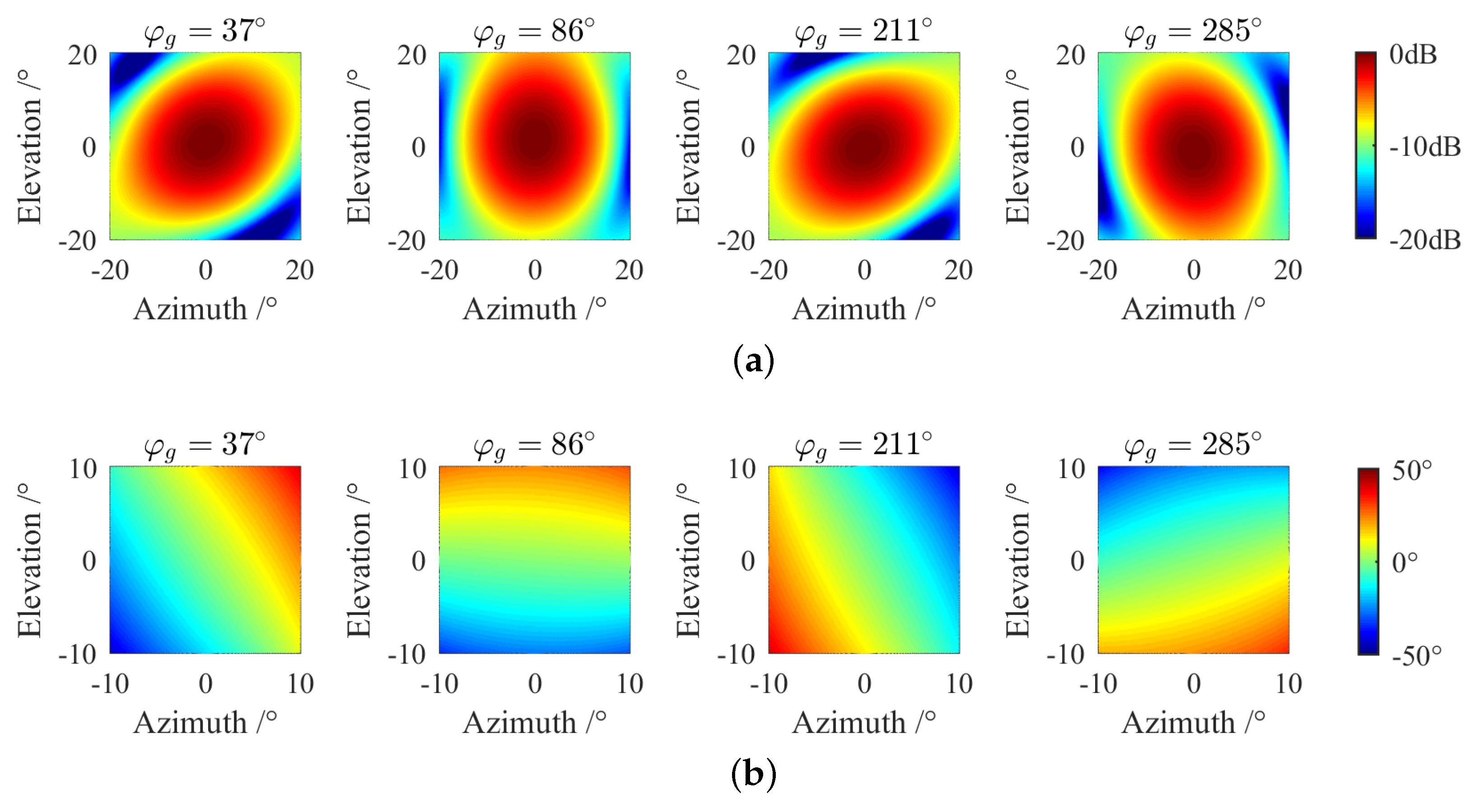
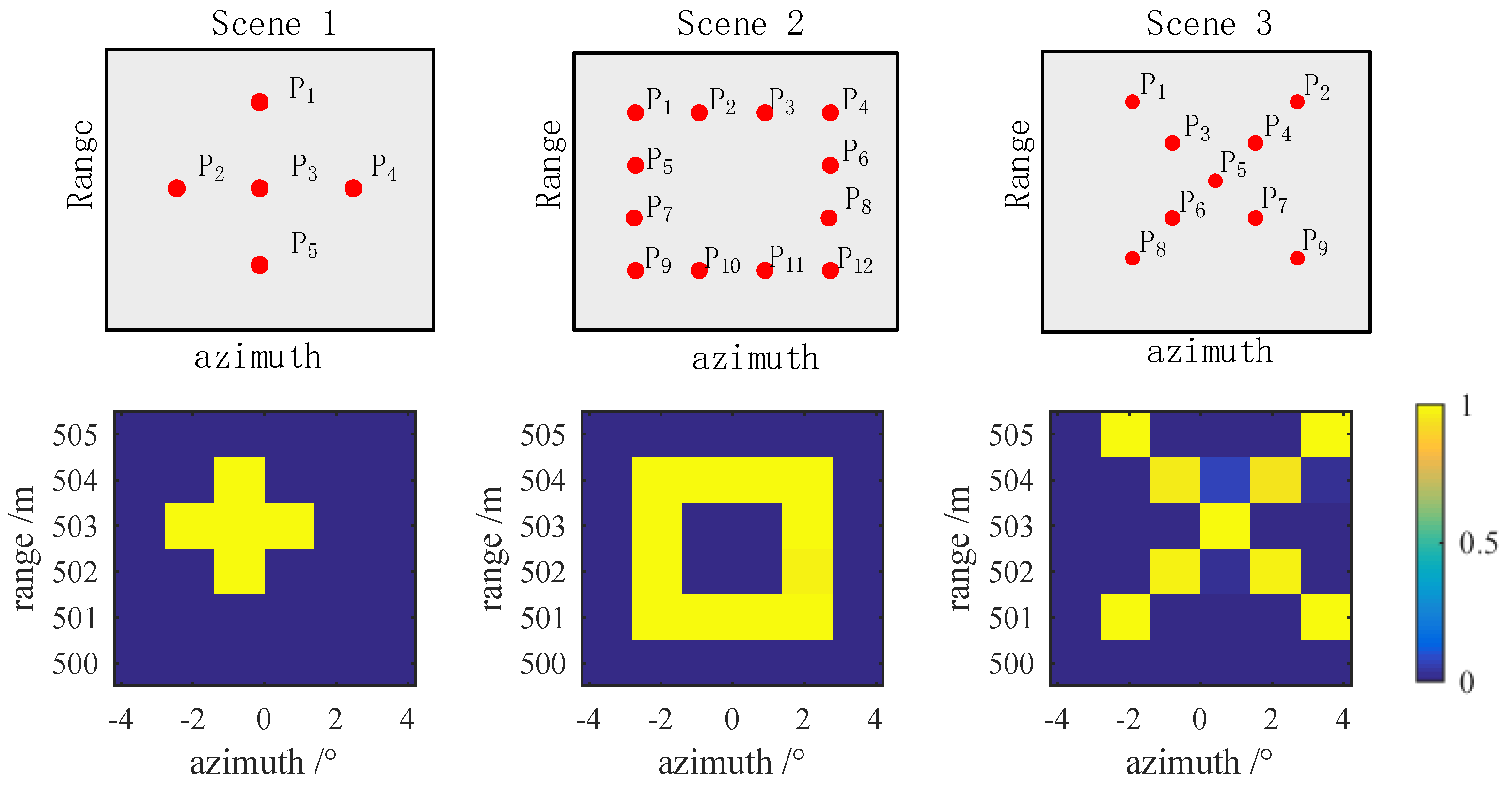
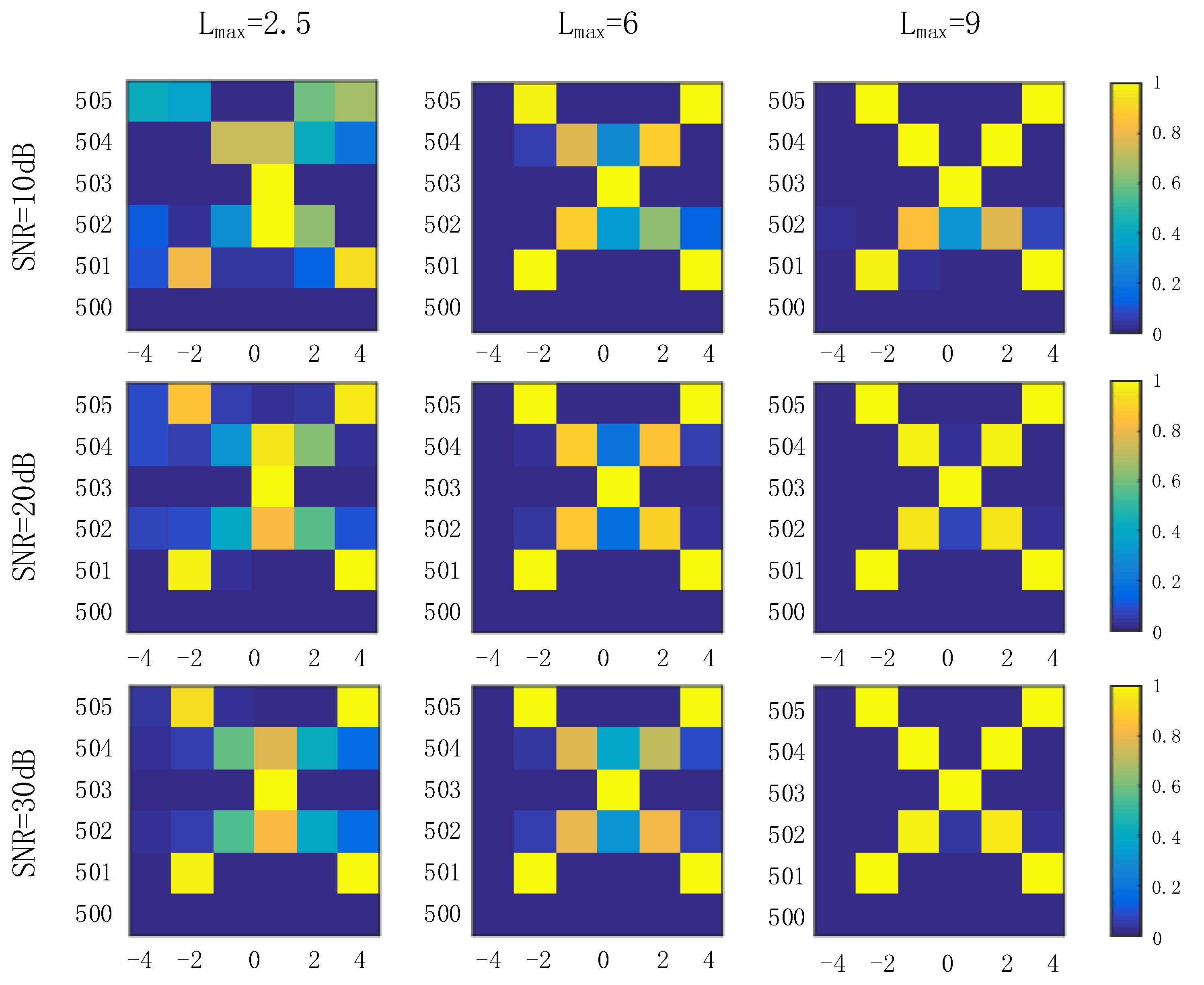
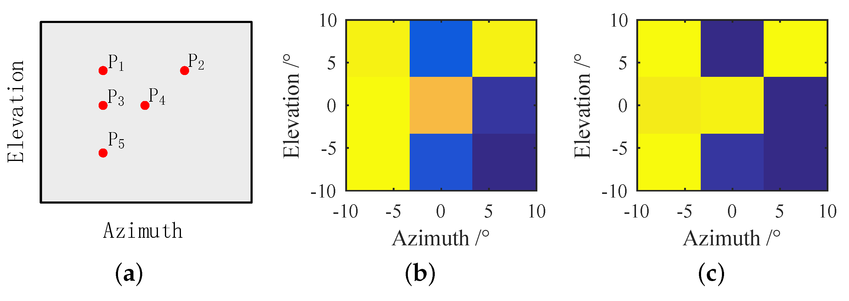
3. Simulation and Discussion

3.1. Two-Dimensional Imaging Simulations Based on the Linear Array

Numerical simulations are conducted to demonstrate the proposed method and to analyze the imaging performance. First, the simulations of the range-azimuth forward-looking imaging based on the linear array is performed. The azimuth resolution is related to the correlation of the measurement matrix H. As the phase gradient of the modulated field increases, the correlation between each row of matrix H decreases. The higher azimuth resolution could be obtained. In the imaging simulations, the azimuth direction of the main lobe is divided into $M=6$ imaging grids. The parameters of the linear array are the same as Section 2.1. $D=6$ modulated fields with phase gradient $L=\pm 9$, $\pm 6$, $\pm 3$ along azimuth direction were constructed for imaging. The beam width ${\theta }_{bw}$ is $7^{\circ }$, and the azimuth resolution, as well as the interval between the adjacent azimuth image grids, is ${\theta }_{bw}/5$. The bandwidth of the transmitted LFM signal is $B=150$ MHz, and the range resolution is $c/2B=1$ m. Figure 7 shows the imaging simulation results of three different scattering point distributions, and the coordinates of each scattering point are shown in

Table 3. Partial scattering point coordinates $(r,\alpha )$ of different imaging scenes.

	Scene 1	Scene 2	Scene 3
$P_1$	$(504$ m, $-{0.7}^{\circ })$	$(504$ m, $-{2.1}^{\circ })$	$(505$ m, $-{2.1}^{\circ })$
$P_2$	$(503$ m, $-{2.1}^{\circ })$	$(504$ m, $-{0.7}^{\circ })$	$(505$ m, $+{3.5}^{\circ })$
$P_3$	$(503$ m, $-{0.7}^{\circ })$	$(504$ m, $+{0.7}^{\circ })$	$(504$ m, $-{0.7}^{\circ })$
$P_4$	$(503$ m, $+{0.7}^{\circ })$	$(504$ m, $+{2.1}^{\circ })$	$(504$ m, $+{2.1}^{\circ })$
$P_5$	$(502$ m, $-{0.7}^{\circ })$	$(503$ m, $-{2.1}^{\circ })$	$(503$ m, $+{0.7}^{\circ })$

. In imaging scene 2, $P_7$ to $P_{12}$ are symmetrically distributed with $P_1$ to $P_6$. In imaging scene 3, $P_6$ to $P_9$ are symmetrically distributed with $P_1$ to $P_4$. The normalized theoretical RCS of the scattering points are 1. Under the condition of signal-to-noise ratio SNR = 20 dB, the estimated RCS of the scattering points are $1\pm 0.04$, and the noise values of the grids without scattering points are less than 0.06. Figure 8 shows the image reconstruction results when the scattering points have different RCS. In imaging scene 1, the RCS of $P_3$ is 1, and the RCS of the rest scattering points is 0.8. In imaging scene 2, the RCS of $P_1$, $P_4$, $P_9$, $P_{12}$ is 1, and the RCS of the rest scattering points is 0.6. The estimated values $\widehat{\sigma }$ of partial scattering points are shown in

Table 4. Partial RCS estimation results of the scattering points.

	Scene 1			Scene 2
	Coordinate	Theoretical	Estimated	Coordinate	Theoretical	Estimated
$P_1$	$(504$ m, $-{0.7}^{\circ })$	0.8	0.79	$(504$ m, $-{2.1}^{\circ })$	1.0	0.97
$P_2$	$(503$ m, $-{2.1}^{\circ })$	0.8	0.78	$(504$ m, $-{0.7}^{\circ })$	0.6	0.61
$P_3$	$(503$ m, $-{0.7}^{\circ })$	1.0	1.02	$(504$ m, $+{0.7}^{\circ })$	0.6	0.61
$P_4$	$(503$ m, $+{0.7}^{\circ })$	0.8	0.78	$(504$ m, $+{2.1}^{\circ })$	1.0	1.01
$P_5$	$(502$ m, $-{0.7}^{\circ })$	0.8	0.80	$(503$ m, $-{2.1}^{\circ })$	0.6	0.59

. The estimated RCS of the scattering points are $1\pm 0.03$, $0.8\pm 0.02$, $0.6\pm 0.03$, and the noise values are less than 0.02.

The imaging performance of the proposed method is affected by the maximum phase gradient $\left(L_{max}\right)$ of the modulated field and the scattering points SNR. For the scattering points distribution the same as scene 3 in Figure 6, the modulated fields with phase gradients $\pm L_{max}/3$, $\pm 2L_{max}/3$, and $\pm L_{max}$ were constructed for imaging. Figure 9 shows the image reconstruction results when the SNR = 10, 20, 30 dB and the maximum phase gradient $L_{max}=2.5$, 6, 9. When the $\mathrm{SNR}=10$ dB and $L_{max}=2.5$, the image reconstruction result is seriously distorted. RCS of partial scattering points are estimated incorrectly. When the maximum phase gradient increases to $L_{max}=9$, the imaging performance are significantly improved. When SNR = 30 dB, the estimated RCS of scattering points are $1\pm 0.04$, and the noise values of the grids without scattering points are less than 0.03.

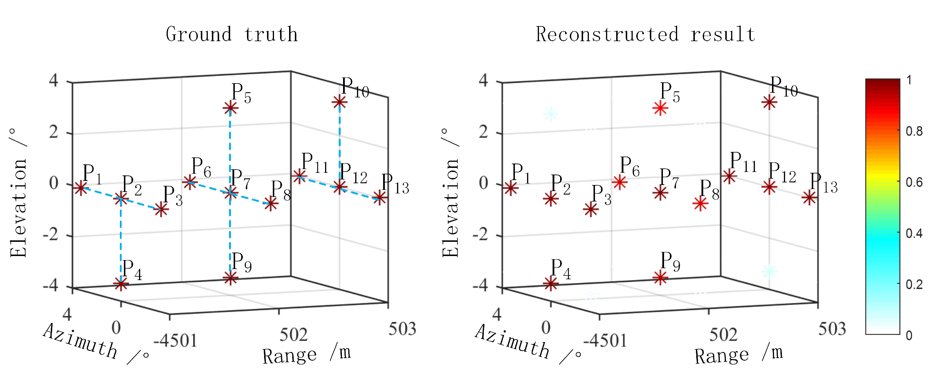
3.2. Three-Dimensional Imaging Simulations Based on the Circular Array

The modulated field constructed by a circular array could distinguish the azimuth and elevation positions of the scattering points at the same range. Firstly, the azimuth-elevation imaging with the scattering points all located at the same range is simulated and analyzed. The parameters of the circular array are the same as Section 2.2. The coordinates $\left(\alpha ,\beta \right)$ of 5 scattering points at the same range are $P_1\left(-{6.6}^{\circ },+{6.6}^{\circ }\right)$, $P_2\left({6.6}^{\circ },+{6.6}^{\circ }\right)$, $P_3\left(-{6.6}^{\circ },0^{\circ }\right)$, $P_4\left(0^{\circ },0^{\circ }\right)$, $P_5\left(-{6.6}^{\circ },-{6.6}^{\circ }\right)$. The RCS of all scattering points are 1. The main lobe is divided into $3\times 3$ discrete grids in azimuth and elevation, and the azimuth and elevation resolution is ${\theta }_{bw}/3$. $D=9$ modulated fields with the same phase gradient value L and different directions ${\phi }_g={24}^{\circ }$, ${37}^{\circ }$, ${62}^{\circ }$, ${86}^{\circ }$, ${136}^{\circ }$, ${161}^{\circ }$, ${211}^{\circ }$, ${235}^{\circ }$, ${285}^{\circ }$ were constructed for imaging. Figure 10 shows the reconstructed results with the phase gradient $L=1$ and 2.5, respectively. When the phase gradient $L=1$, the correlation between each row of H is relatively strong, and the RCS estimation error of the scattering points is large. The estimated RCS of scattering points are $1\pm 0.18$, and the maximum value of noise is 0.12. When the phase gradient $L=2.5$, the correlation of the measurement matrix H decreases, and the imaging performance is improved. The estimated RCS of the scattering points are $1\pm 0.07$, and the noise values are less than 0.03.

When the ranges of the scattering points are different, the simulation results of range-azimuth-elevation three-dimensional imaging are shown in Figure 11. The coordinates of each scattering point are shown in

Table 5. Coordinates and estimated RCS of the scattering points.

	Coordinate	RCS $\mathit{\sigma }$			Coordinate	RCS $\mathit{\sigma }$
	$(\mathit{r},\mathit{\alpha },\mathit{\beta })$	Theoretical	Estimated		$(\mathit{r},\mathit{\alpha },\mathit{\beta })$	Theoretical	Estimated
$P_1$	$\left(501 \mathrm{m},+{3.3}^{\circ },0^{\circ }\right)$	1	1.02	$P_8$	$\left(502 \mathrm{m},-{3.3}^{\circ },0^{\circ }\right)$	1	0.91
$P_2$	$\left(501 \mathrm{m},0^{\circ },0^{\circ }\right)$	1	1.01	$P_9$	$\left(502 \mathrm{m},0^{\circ },-{3.3}^{\circ }\right)$	1	0.95
$P_3$	$\left(501 \mathrm{m},-{3.3}^{\circ },0^{\circ }\right)$	1	1.00	$P_{10}$	$\left(503 \mathrm{m},0^{\circ },+{3.3}^{\circ }\right)$	1	1.10
$P_4$	$\left(501 \mathrm{m},0^{\circ },-{3.3}^{\circ }\right)$	1	1.08	$P_{11}$	$\left(503 \mathrm{m},+{3.3}^{\circ },0^{\circ }\right)$	1	1.08
$P_5$	$\left(502 \mathrm{m},0^{\circ },+{3.3}^{\circ }\right)$	1	0.88	$P_{12}$	$\left(503 \mathrm{m},0^{\circ },0^{\circ }\right)$	1	0.97
$P_6$	$\left(502 \mathrm{m},+{3.3}^{\circ },0^{\circ }\right)$	1	0.92	$P_{13}$	$\left(503 \mathrm{m},-{3.3}^{\circ },0^{\circ }\right)$	1	1.08
$P_7$	$\left(502 \mathrm{m},0^{\circ },0^{\circ }\right)$	1	1.00

. The bandwidth of the LFM signal is 150 MHz. The scattering points at different ranges are distinguished by LFM signal pulse compression. The azimuth and elevation directions are divided into 3 × 3 imaging grids for image reconstruction. Under the condition of SNR = 20 dB, the estimated RCS of each scattering point are shown in Table 5. The estimated RCS of the scattering points are $1\pm 0.12$, and the noise values are less than 0.08.

4. Conclusions

In this paper, we proposed a forward-looking method by constructing the modulated field with linear wavefront. The linear wavefront could be adjusted by the amplitude coefficients of the antenna array units. The modulated fields could generate linear phase changes along azimuth and elevation directions simultaneously. The two-dimensional and three-dimensional forward-looking imaging could be achieved by the linear and the circular array, respectively. In multiple simulation experiments under the condition of SNR = 20 dB, the image can be accurately reconstructed by the proposed method. Compared with vortex electromagnetic waves, the modulated field has the maximum radiation intensity at the center of the beam. The beam divergence is avoided and no beam collimation is required for imaging. The proposed imaging method based on modulated fields has potential applications in the fields of target recognition and autonomous driving of unmanned vehicles.

References

1. Sroor, H.; Huang, Y.W.; Sephton, B.; Naidoo, D.; Vallés, A.; Ginis, V.; Qiu, C.W.; Ambrosio, A.; Capasso, F.; Forbes, A. High-purity orbital angular momentum states from a visible metasurface laser. Nat. Photonics 2020, 14, 498–503. [Google Scholar] [CrossRef]
2. Feng, P.Y.; Qu, S.W.; Yang, S. OAM-Generating Transmitarray Antenna With Circular Phased Array Antenna Feed. IEEE Trans. Antennas Propag. 2020, 68, 4540–4548. [Google Scholar] [CrossRef]
3. Yan, Y.; Xie, G.; Lavery, M.P.J.; Huang, H.; Ahmed, N.; Bao, C.; Ren, Y.; Cao, Y.; Li, L.; Zhao, Z.; et al. High-capacity millimetre-wave communications with orbital angular momentum multiplexing. Nat. Commun. 2014, 5, 4876. [Google Scholar] [CrossRef] [PubMed] [Green Version]
4. Bozinovic, N.; Yue, Y.; Ren, Y.; Tur, M.; Kristensen, P.; Huang, H.; Willner, A.E.; Ramachandran, S. Terabit-Scale Orbital Angular Momentum Mode Division Multiplexing in Fibers. Science 2013, 340, 1545–1548. [Google Scholar] [CrossRef] [Green Version]
5. Lavery, M.; Speirits, F.; Barnett, S.M.; Padgett, M.J. Detection of a Spinning Object Using Light’s Orbital Angular Momentum. Science 2013, 341, 537–540. [Google Scholar] [CrossRef] [Green Version]
6. Lavery, M.P.J.; Barnett, S.M.; Speirits, F.C.; Padgett, M.J. Observation of the rotational Doppler shift of a white-light, orbital-angular-momentum-carrying beam backscattered from a rotating body. Optica 2014, 1, 1–4. [Google Scholar] [CrossRef]
7. Luo, Y.; Chen, Y.J.; Zhu, Y.Z.; Li, W.Y.; Zhang, Q. Doppler effect and micro-Doppler effect of vortex-electromagnetic-wave-based radar. IET Radar Sonar Navig. 2020, 14, 2–9. [Google Scholar] [CrossRef]
8. Cheng, Y.; Wang, H.; Qin, Y.l.; Fan, B. Radar imaging using electromagnetic wave carrying orbital angular momentum. J. Electron. Imaging 2017, 26, 023016. [Google Scholar]
9. Liu, H.; Liu, K.; Cheng, Y.; Wang, H. Microwave Vortex Imaging Based on Dual Coupled OAM Beams. IEEE Sens. J. 2020, 20, 806–815. [Google Scholar] [CrossRef]
10. Liu, H.; Wang, Y.; Wang, J.; Liu, K.; Wang, H. Electromagnetic Vortex Enhanced Imaging Using Fractional OAM Beams. IEEE Antennas Wirel. Propag. Lett. 2021, 20, 948–952. [Google Scholar] [CrossRef]
11. Wang, H.; Cheng, Y.; Qin, Y.l. Electromagnetic Vortex-Based Radar Imaging Using a Single Receiving Antenna: Theory and Experimental Results. Sensors 2017, 17, 630. [Google Scholar] [CrossRef] [Green Version]
12. Liu, K.; Li, X.; Gao, Y.; Wang, H.; Cheng, Y. Microwave imaging of spinning object using orbital angular momentum. J. Appl. Phys. 2017, 122, 124903. [Google Scholar] [CrossRef]
13. Liu, K.; Cheng, Y.; Wang, H.; Li, X.; Qin, Y. Radiation pattern synthesis for the generation of vortex electromagnetic wave. IET Microw. Antennas Propag. 2017, 11, 685–694. [Google Scholar] [CrossRef]
14. Liu, K.; Cheng, Y.; Yang, Z.; Wang, H.; Qin, Y.; Li, X. Orbital-Angular-Momentum-Based Electromagnetic Vortex Imaging. IEEE Antennas Wirel. Propag. Lett. 2015, 14, 711–714. [Google Scholar] [CrossRef]
15. Yuan, T.; Cheng, Y.; Wang, H.; Qin, Y. Beam Steering for Electromagnetic Vortex Imaging Using Uniform Circular Arrays. IEEE Antennas Wirel. Propag. Lett. 2017, 16, 704–707. [Google Scholar] [CrossRef]
16. Yuan, T.; Wang, H.; Qin, Y.; Cheng, Y. Electromagnetic Vortex Imaging Using Uniform Concentric Circular Arrays. IEEE Antennas Wirel. Propag. Lett. 2016, 15, 1024–1027. [Google Scholar] [CrossRef]
17. Liu, K.; Cheng, Y.; Li, X.; Qin, Y.; Wang, H.; Jiang, Y. Generation of Orbital Angular Momentum Beams for Electromagnetic Vortex Imaging. IEEE Antennas Wirel. Propag. Lett. 2016, 15, 1873–1876. [Google Scholar] [CrossRef]
18. Qin, Y.; Liu, K.; Cheng, Y.; Li, X.; Wang, H.; Gao, Y. Sidelobe Suppression and Beam Collimation in the Generation of Vortex Electromagnetic Waves for Radar Imaging. IEEE Antennas Wirel. Propag. Lett. 2017, 16, 1289–1292. [Google Scholar] [CrossRef]
19. Liu, K.; Cheng, Y.; Gao, Y.; Li, X.; Qin, Y.; Wang, H. Super-resolution radar imaging based on experimental OAM beams. Appl. Phys. Lett. 2017, 110, 164102. [Google Scholar] [CrossRef]
20. Lin, M.; Gao, Y.; Liu, P.; Liu, J. Super-resolution orbital angular momentum based radar targets detection. Electron. Lett. 2016, 52, 1168–1170. [Google Scholar] [CrossRef]
21. Liu, K.; Li, X.; Gao, Y.; Cheng, Y.; Wang, H.; Qin, Y. High-Resolution Electromagnetic Vortex Imaging Based on Sparse Bayesian Learning. IEEE Sens. J. 2017, 17, 6918–6927. [Google Scholar] [CrossRef]
22. Liu, K.; Cheng, Y.; Liu, H.; Wang, H. Computational imaging with low-order OAM beams at microwave frequencies. Sci. Rep. 2020, 10, 11641. [Google Scholar] [CrossRef] [PubMed]
23. Padgett, M.J.; Miatto, F.M.; Lavery, M.P.J.; Zeilinger, A.; Boyd, R.W. Divergence of an orbital-angular-momentum-carrying beam upon propagation. New J. Phys. 2015, 17, 023011. [Google Scholar] [CrossRef]
24. Lin, M.; Gao, Y.; Liu, P.; Liu, J. Theoretical Analyses and Design of Circular Array to Generate Orbital Angular Momentum. IEEE Trans. Antennas Propag. 2017, 65, 3510–3519. [Google Scholar] [CrossRef]
25. Zhong, Y.; Zhang, Y.; Zhang, X.; Sun, H.; Zhao, G. Velocity measurement of an arbitrary three-dimensional moving object by using a novel modulated field. Opt. Express 2021, 29, 26210–26219. [Google Scholar] [CrossRef]
Figure 1. Linear array antenna.
Electronics 11 02083 g001
Figure 2. The modulated field constructed by the linear array. The amplitude pattern (a) and the phase distributions (b) along the azimuth direction (XOZ plane). (c) The two-dimensional phase distribution within the main lobe.
Electronics 11 02083 g002
Figure 3. Circular array antenna.
Electronics 11 02083 g003
Figure 4. Two-dimensional amplitude and phase distribution of the modulated fields with the phase gradient directions φ g = 37 , 86 , 211 , 285 and gradient value L = 2.5 . (a) Amplitude distribution; (b) phase distribution within main lobe.
Electronics 11 02083 g004
Figure 5. The amplitude and phase patterns in the azimuth direction (XOZ plane) and elevation direction (YOZ) of the modulated fields with φ g = 37 (a), 86 (b), 211 (c), 285 (d) and L = 2.5 .
Electronics 11 02083 g005
Figure 6. The amplitude (a) and phase (b) distributions of the vortex beam ( l = 1 ).
Electronics 11 02083 g006
Figure 7. Range-azimuth two dimensional silumations of different imaging scenes.
Electronics 11 02083 g007
Figure 8. Image reconstruction results when the scattering points have different RCS.
Electronics 11 02083 g008
Figure 9. Imaging performance with different SNR and L m a x .
Electronics 11 02083 g009
Figure 10. Azimuth-elevation image reconstruction results. Ground truth (a). Image reconstruction results with phase gradient L = 1 (b), and L = 2.5 (c).
Electronics 11 02083 g010
Figure 11. Range-azimuth-elevation three-dimensional imaging results.
Electronics 11 02083 g011