Abstract
Deciding binding, routing, and scheduling within system synthesis for hard real-time systems can be a challenging task. Symbolic methods leveraging results from the area of satisfiability modulo theories (SMT) solving have shown to be scalable methods for this by splitting the work between a logic solver for routing and binding, and a background theory solver performing schedulability analysis. For these methods, in order to prune the search space of infeasible implementations efficiently, a feedback by the background theory is required. It can be observed that previous approaches might fail here as feedback cannot be derived within a reasonable amount of time. We propose a coordinated synthesis approach that overcomes this issue. Here, we leverage an answer set solver as logic solver that is enhanced with a scheduling-aware binding and routing refinement. Based on the answer set solver’s decisions for binding and routing, a background theory solver then computes time-triggered schedules to resolve resource access conflicts. If no feasible schedule exists, a feedback to the answer set solver can be derived within reasonable time. Our experiments synthesizing massively parallel hardware architectures show that our approach increases the applicability of symbolic synthesis considerably. While more than half of the investigated instances in our experiments cannot be solved in the non-coordinated approach already at small 2-dimensional tiled mesh hardware architectures with average computational utilization per tile, the coordinated synthesis approach scales up to architectures with average utilization of per tile ( the hardware architecture size than before). Furthermore, we increase the scalability and the robustness of our approach by encoding our domain-knowledge within domain-specific heuristics in our designated answer set solver. Within our experiments, we observe that the domain-specific heuristics enable us to scale up to architectures with average utilization per tile.
1. Introduction
In the process of developing a novel embedded system, developers often start at the electronic system level. During system synthesis, the fundamental design decision binding, routing and scheduling are decided [1]. A binding contains for each computational task of an application model an assignment to a processing element (PE) of a platform model. If information between computational tasks is exchanged via messages, a routing for each message consists of an ordered set of connected hardware resources. Finally, scheduling resolves concurrent access to shared resources by applying a suitable policy.
In recent years, system synthesis has become more and more challenging due to increasing system complexity. Concerning the automotive domain, one major contribution to this complexity are parallel hardware architectures. These parallel architectures have become a necessity in the control-dominated systems in the automotive industry in order to meet performance requirements, e.g., due to customer demands for new features or the need to implement sophisticated algorithms to meet environmental goals.
While multi-core architectures offer enough performance to realize the currently requested requirements [2], many-core architectures will become necessary in the foreseeable future. Regarding the interconnect implemented by these hardware architectures, it is likely that one or more network-on-chip (NoC) interconnects are a reasonable choice as they scale well with an increasing number of PEs and are very power-efficient [3,4].
Despite that many-core architectures with NoCs offer scalable performance, they introduce a new set of challenges for system synthesis in control-dominated domains like the automotive domain. First of all, synthesis approaches have to handle a significant increase in the number of entities for which binding, routing and scheduling have to be decided. Additionally, and most of the time far more challenging, the timing constraints of automotive hard real-time applications have to be satisfied. Here, satisfying the timing constraints becomes a considerably challenging task if system specifications become more intricate and decisions during synthesis become interdependent. As manual approaches are likely to fail in this setting, symbolic approaches based on satisfiability modulo theories (SMT) emerged as scalable automated decision making approaches in the area of system synthesis, e.g., [5,6,7].
In SMT-based system synthesis, the workload of synthesis is split between a logic solver and a background theory solver (-solver), see Figure 1. This decoupling enables more scalable symbolic synthesis for hard real-time systems [6].
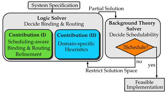
Figure 1.
Overview of the contributions within the symbolic system synthesis approach presented in this paper.
In the paper at hand, similar to [6], the logic solver decides the binding of computational tasks to PEs of the hardware architecture and the multi-hop routing of messages. These decisions are then the input for the -solver in order to decide schedulability of the logic solver’s assignments. Thus, the solution space for the -solver is constrained. If the -solver proves that there exists no feasible schedule with respect to the decided binding and routing, the background theory computes a feedback that allows to prune the search space of the logic solver. With this feedback, the SMT-based synthesis is able to learn infeasible solutions and therefore is able to avoid them in the subsequent search process.
Unfortunately, as we will show in the experimental section (Section 8) of this paper, one can observe that deciding schedulability based on the logic solver’s decisions might consume an excessive amount of time if the logic solver is allowed to perform its decisions in arbitrary orders and particularly without knowledge of the downstream scheduling task. As a result, the feedback of the background theory is considerably deferred, hence limiting the applicability and scalability of SMT-based system synthesis.
As a remedy, Figure 1 highlights the main contributions of our work that enable us to realize and significantly increase the applicability, scalability and robustness of SMT-based system synthesis:
- (I)
- We present a coordinated SMT-based synthesis approach that eases the task of the -solver to compute a feedback to the logic solver. This is realized by introducing a scheduling-aware binding and routing refinement in the logic solver.
- (II)
- We present how domain-specific heuristics (DSH) applied within the logic solver allow us to further increase scalability of our approach by utilizing our domain knowledge.
In our experimental evaluation, we show that both our contributions on the one hand significantly increase applicability and on the other hand considerably enhance scalability of SMT-based system synthesis. Here, our instance sets leverage an automotive domain oriented application model that comprises both serial and parallel characteristics, namely two-terminal series-parallel task graphs [8]. Hence, we address an application model suitable for future parallel hardware architectures due to inclusion of the fork-join pattern. However, at the same time, we respect the more sequential processing characteristics of today’s control applications with a not-negligible length of chained tasks in the series-parallel task graphs.
The remainder of this paper is structured as follows: Section 2 explains the concepts and limitations of current SMT-based approaches in detail and motivates our contributions. In Section 3, we summarize related work while Section 4 introduces our platform and application model. We summarize how our approach leverages answer set programming (ASP) as logic solver in Section 5 and briefly illustrate the relevant points of our time-triggered scheduling formulation within the background theory in Section 6. Section 7 explains how we couple the logic solver and the background theory in order to derive the feedback to prune the search space of the logic solver efficiently. Our experimental results in Section 8 demonstrate that our coordinated approach can improve the applicability of symbolic system synthesis considerably and that our DSH allow to increase the scalability and robustness of our approach. Section 9 finalizes this paper by proving concluding remarks.
2. Coordinated SMT-Based Synthesis Approach: Motivation & Detailed Overview
In this section we present a succinct summary of the integral parts of our SMT-based system synthesis implementation. We start with introducing state-of-the-art classical SMT-based system synthesis, which is similar to work presented in [5,6,7,9,10]. Then, we sketch the obstacles that motivated us to integrate our extensions in order to realize our proposed coordinated synthesis approach.
2.1. (Classical) SMT-Based System Synthesis
Figure 2 illustrates the elements of SMT-based synthesis. For the classical synthesis approach, all shown elements are vital, except the two boxes in green and cyan, those are part of our extension within the coordinated synthesis approach.
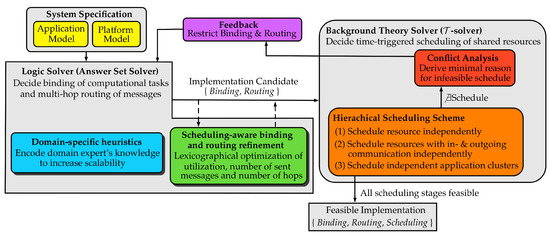
Figure 2.
Detailed overview of SMT-based system synthesis with the extensions of the scheduling-aware binding and routing refinement (green box) in the coordinated synthesis approach and the coordinated+DSH approach (green and cyan box).
The system specification is the starting point. It consists both of an instance of our application model and platform model (yellow boxes in Figure 2) for which we decide a binding, routing and scheduling during synthesis. Our platform model focuses on scalable tile-based architectures implementing a NoC [4]. Furthermore, our graph-based application model is geared to real-world periodic control applications with hard real-time constraints from the automotive domain.
The system specification is an input for the logic solver which decides the static binding of periodic computational tasks from the application model to processing elements (PEs) of the platform model. Furthermore, the logic solver computes the static multi-hop routing of periodic messages between computational tasks. It is important to note that our synthesis approach employs an answer set solver from the area of answer set programming (ASP) [11,12,13] as logic solver in contrast to most related approaches that use a Pseudo-Boolean SAT solver for the same task. Here, related work [14] encouraged us to favor an answer set solver since ASP allows a more scalable determination of multi-hop routes of messages for densely connected hardware architectures implementing a NoC.
With the logic solver computing a binding and routing implementation candidate, this solution is subsequently passed to the -solver for a scheduling analysis. Here, scheduling instances are generated on basis of indicator variables that have an interpretation in both the logic solver as in the -solver. These indicator variables are also used to express feedback of the -solver to the logic solver in order to learn unschedulable bindings and routings. In our approach, the indicator variables correspond to the binding of a computational task to a PE and the hops in the route of a message.
Deciding the scheduling in the background theory solver to resolve resource access conflicts assumes a time-triggered scheduling policy on all resources of the hardware platform. Here, each computational task on a PE and each packet of a message on each resource on the message’s route through the NoC is assigned a dedicated start time. At this start time, the resource starts the associated computations or the transfer of a packet. The -solver decides whether a time-triggered schedule exists such that all timing constraints of computational tasks and messages are satisfied. If a schedule exists for all computational tasks and all messages based on the logic solver’s binding and routing decisions, the synthesis stops and returns a feasible implementation.
However, in the first iteration of SMT-based synthesis approaches it is unlikely that the background theory will find a feasible scheduling right at the start. Usually, the -solver proves that early bindings and routes computed by the logic solver cannot be scheduled. Similar to other work [7], in order to speed up the time to decide schedulability, we propose a hierarchical scheduling scheme (orange box in Figure 2). In our hierarchical scheduling scheme, the -solver decides feasibility of smaller sub-problems before the feasibility of the scheduling for the complete system is decided. Usually proving the infeasibility of small sub-problems is much faster than proving the infeasibility of the complete system scheduling. If a sub-problem is already deemed infeasible it follows that the complete system cannot be scheduled. In Section 7 we will introduce the hierarchical scheduling stages in detail.
If the background theory solver proves that a scheduling (sub-)problem cannot be solved, a subsequent conflict analysis (red box in Figure 2) is started. Here, we also benefit from the hierarchical scheduling scheme as it usually speeds up the conflict analysis since smaller sub-problems have to be analyzed. During conflict analysis, an minimal unsatisfiable core (or justification, unsatisfiable core or irreducible inconsistent subset) [15] is derived why no time-triggered schedule exists. For example, assume a schedule cannot be derived for a PE with five computational tasks bound to it. However, the minimal unsatisfiable core for the conflict could be that only two of these tasks prevent scheduling due to their timing parameters. All combinations including both two tasks are thus infeasible. And this is also true for bindings, which have not been seen up to this point. Related work [6] has shown that deriving a minimal unsatisfiable cores in a conflict analysis can significantly speed up the scalability of symbolic system synthesis as it can enable an extensive pruning of the logic solver’s search space. Revisiting our previous example, all solutions where the two conflicting computational tasks are bound to the same PE will not result in a feasible implementation and should therefore be excluded in the search space of the logic solver.
Thus, a feedback to the logic solver is generated that restricts the subsequent binding and routing solutions of the logic solver (purple box in Figure 2). Here, as mentioned earlier, the indicator variables are used to constrain the search space by adding so-called integrity constraints to the set of rules of the logic solver (see Section 5). All following binding and routing implementation solution candidates will avoid all conflicts from the background theory that have been learned so far. The iterative coupling between logic solver and -solver stops with a successfully hierarchical scheduling or if the logic solver returns the result UNSAT (unsatisfiable). In the latter case the SMT-based synthesis approach proved that there exists no feasible implementation with respect to the system’s specification.
Regrading the complexity of the system specifications that the classical approach is able to synthesize, this approach can face serious applicability issues, as we will see later within our experimental section (Section 8). This is due to the often very complex and time consuming time-triggered scheduling analysis within the background theory solver. The upper timeline in Figure 3 illustrates the observation that is usually made.
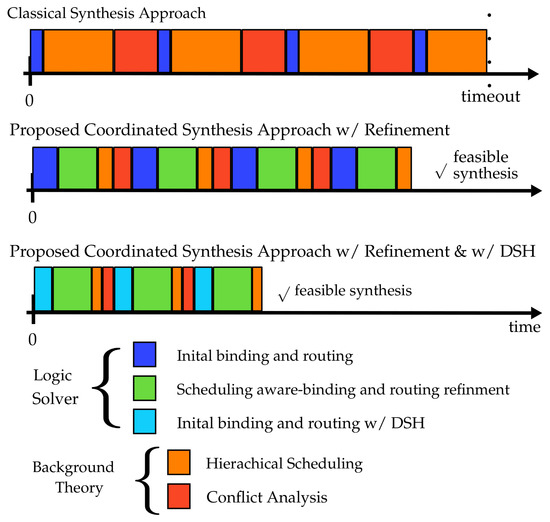
Figure 3.
Illustration of the disadvantages of the classical synthesis approach along wit the advantages of the coordinated and coordinated+DSH approach. The classical approach spends a considerable amount of time within the background theory until reaching a timeout. The coordinated synthesis approach significantly increases the applicability of symbolic system synthesis by introducing an additional scheduling-aware binding and rounting refinement. The coordinated+DSH approach, which includes domain-specific heuristics (DSH) in the logic solver, furthermore increases the scalability of the coordinated approach and reduces the average synthesis time, too.
Here, the logic solver is able to compute a binding and routing solution within a very short amount of time (blue box in Figure 3), often even within milliseconds. However, the subsequent scheduling analysis and conflict analysis (orange and red boxes in Figure 3) are very time consuming and several magnitudes higher than the time spent in the logic solver. Hence, the necessary feedback from the -solver to the logic solver cannot be derived within a reasonable amount of time which can ultimately limit the applicability of classical SMT-based system synthesis. Usually, the classical approach is stopped after a certain timeout without providing a solution to the synthesis problem (see experiments in Section 8).
As a remedy, we propose a coordinated SMT-based synthesis approach with the logic solver computing a binding and routing solution such that the -solver is able to decide feasibility within a reasonable amount of time.
2.2. Coordinated SMT-Based System Synthesis
In the work at hand, we realize the coordination between logic solver and background theory solver by introducing a scheduling-aware binding and routing refinement (highlighted green in Figure 2) in the logic solver. With the scheduling-aware binding and routing refinement, the logic solver is assigned an additional fixed amount of time to solely perform an lexicographical optimization of an initially derived binding and routing solution. Here, the optimization includes load balancing and a minimization of both the number of sent messages by computational tasks and the overall number of hops of messages in the routing. In contrast to the initial solution, that can be compared to the binding and routing solutions computed in the classical approach, the -solver is expected to decide feasibility and perform a conflict analysis on the refined solutions within a reasonable amount of time, as shown in the timeline in the middle of Figure 3 (orange and red boxes). This comes with the cost that now more time is spent in the logic solver during synthesis. On the one hand, this is due to the additional time assigned for the refinement of an initial binding and routing solution (green boxes in Figure 3). On the other hand, additional rules are necessary to realize the refinement’s objectives which results in larger instances for the logic solver. For the hardest system specifications we consider in this paper (see Section 8), this results in an increase of up to in the number of variables and up to in the number of constraints in the logic solver. Thus we observe a larger blue box for the coordinated approach in Figure 3. Nevertheless, despite the additional effort for the logic solver (blue and green box in Figure 3), the coordinated SMT-based synthesis significantly increases the applicability of SMT-based system synthesis as we will show in the experimental section.
2.3. Increasing Scalability of Coordinated SMT-Based Synthesis by Domain-Specific Heuristics
Despite the significant increase in applicability of SMT-based synthesis that can be achieved with a coordinated approach, another significant gain in scalability and robustness of the approach can be realized if one leverages exclusive domain knowledge. In this paper we incorporate our domain knowledge by enriching the state-of-the-art search heuristic in the logic solver by domain-specific heuristics (DSH) (cf. cyan box in Figure 2). Here, we use particular heuristic predicates within the modeling language of our designated logic solver, the answer set solver clasp [16,17], to express our domain knowledge based on the system’s specification (see Section 5). We integrate the DSH together with the scheduling-aware binding and routing refinement that form the novel coordinated+DSH synthesis approach. While this approach does not only lead to a decrease in the average time spent in the logic solver as well as in the background theory (see Figure 3), we further increase the scalability of the coordinated approach considerably (see experiments in Section 8).
3. Related Work
To keep up with the increasing complexity of system specification, symbolic system synthesis approaches based on Pseudo-Boolean satisfiability (PB-SAT), e.g., [18], emerged as solutions to handle challenging system specifications where previous (meta-)heuristic approaches may fail. While these methods are able to efficiently restrict parts of the infeasible search space, they are mostly limited to linear constraints and potential binary encodings of integer domains tend to an exponential growth in variables. As a remedy, to handle non-linear functional constraints such as hard real-time timing constraints which require large numeric domains, new symbolic synthesis approaches leverage results form the area of satisfiability modulo theories (SMT) solving [15,19]. Thereby, SMT solvers decide the satisfiability of decision problems on logical formulae and these formulae are then interpreted by background theories. In a lot of approaches the propositional part of an SMT solver is realized by a SAT solver whereas a solution with respect to the background theory is computed by a so-called -solver.
As one of the first publications regarding SMT-based system synthesis, the authors in [20] make use of the SMT-solving’s decomposition principle to increase the scalability. Here, the -solver solves a graph-theoretic sub-problem. In [21] latency computation is used for scheduling analysis in the -solver and the authors were able to increase performance more than an order of magnitude. Similar to our time-triggered scheduling model, the work of [22] presents an SMT-based with linear arithmetic for adding worst-case execution times within the background theory. While all the work above are SMT-based approaches, they do not incorporate the multi-hop routing and scheduling of messages.
Fundamental work in SMT-based system synthesis also including the computation of multi-hop routes has been done by Reimann et al. [5]. The authors use Modular Performance Analysis (MPA) in combination with Real-Time Calculus [23] for timing analysis in the background theory. Furthermore, the work in [5] shows that analyzing partial models, i.e., checking parts of the proposed full binding and routing solution, outperforms existing approaches. The same authors further increase the performance of their approach in [6] by deducing justifications (i.e., reasons why a task violates its deadline) within the background theory to prune the search space of their SAT-solver more efficiently. With these extensions, the speed-up in time to derive a feasible system synthesis in their case studies ranges from a factor of 10× up to more than 160×. The approach of deducing a justification is based on analyzing the critical path set of a computational task t which violates its deadline. The critical path set is defined by all computational tasks or messages that are predecessors of task t in the same application graph. In contrast to the work at hand, the authors do not incorporate a hierarchical scheduling scheme, e.g., starting with scheduling all computational tasks on the same resource independently, which could lead to smaller justifications (in terms of variables) and hence a more efficient pruning of infeasible search space. Additionally, the derived justifications are not necessarily minimal as no filter algorithm is implemented to derive minimal unsatisfiable cores (see Section 7).
Kumar et al. [10] build on the same -solver like [5,6] but also consider delay, buffer and energy constraints of incomplete models. By using incomplete models, the variables of bindings and multi-hop routings proposed to the -solver are only partially assigned other than required by the system specification. As a benefit, infeasible regions of the search space can be pruned more efficiently which considerably enhances the capabilities of symbolic synthesis to prove the absence of feasible system implementations.
Lukasiewycz and Chakraborty [7] present an SMT-based architecture optimization and scheduling approach. While they focus on time-triggered automotive bus systems, the authors implement several techniques that are also used within the work at hand, e.g., a hierarchical scheduling scheme to increase performance.
All the work discussed above leverages (PB-)SAT-solvers as logic solvers in their SMT-based approaches. In [14], Andres et al. show that using answer set programming (ASP) [11,13] has advantages for highly connected architectures. While their work does not include a background theory to decide scheduling, their work shows that deciding the multi-hop routes of messages is more scalable for NoC-based architectures. Hence, their work encouraged us to leverage ASP to decide the binding and multi-hop routing in our synthesis approach.
Regarding ASP and a coupling to a background theory for system synthesis, Neubauer et al. [9] tightly couple answer set programming with the same background theory as in this paper for scheduling analysis. By leveraging technical advances in a new version of the answer set solver clingo [24] the authors are able to analyze incomplete models which was not possible at the time we developed our coordinated approach. An additional difference to our work is that the authors do not use a hierarchical scheduling scheme and do not investigate the influence of domain-specific heuristics (DSH) in their approach. Furthermore, the experiments in [9] indicate that our coordinated approach based on partial models can have advantages w.r.t. the total synthesis time for feasible system specifications.
An extension of the work in [9] can be found in [25]. While the same limitations in comparison to our work exist as in [9], the novelty of [25] lies in the integration of a multi-objective optimization into the background theory allowing for an automatic design space exploration. This extension is orthogonal to our work.
Note that all related work presented above does not consider a coordination between the logic solver and the background theory. As we will show in our experimental section (cf. Section 8), an approach without coordination considerably suffers applicability as the feedback by the -solver might not be provided within a reasonable amount of time. Furthermore, we investigate how symbolic system synthesis can be enhanced by domain-specific heuristics within the logic solver in order to increase scalability and robustness.
Our approach is based on previous preliminary work [26,27] that has been extended with refinements in several directions. The work at hand uses a portfolio solving approach in the background theory (see Section 8.2), also in order to show that the classical approach does only scale to a certain limit even if different strategies and configurations are used within the background theory. Additionally, a scheduling constraint within the logic solver (the so-called Korst-constraint, see Section 5) considerably reduces couplings between logic solver and background theory and, to the best of our knowledge, has not been implemented in related symbolic synthesis approaches before. Regarding the modeling of more realistic applications, e.g., from the automotive domain, our application model is based on two terminal series-parallel (TTSP) application graphs [28] that capturing characteristics of today’s and future automotive software for (massively) parallel hardware architectures. In our experiments, we evaluated our approach on considerably harder benchmarking instances incorporating TTSP application graphs as compared to [26,27].
4. System Model
In this section, we introduce our formal system model which builds the foundation of the remainder of this paper. Furthermore, we provide a formal problem formulation based on the introduced system model.
4.1. Platform Model
Our platform model is a versatile abstract model which enables modeling of several crucial aspects of heterogeneous parallel architectures, e.g., inhomogeneous performance of processing elements and the on-chip communication infrastructure. Since tile-based architectures interconnected by a NoC are considered to be a scalable reference design for massively parallel hardware platforms [3,4], these type of platforms are of our special interest and therefore in the main focus of our platform model.
We model the topology of tile-based many-core hardware platforms as a directed graph , the platform graph.
The platform graph’s set of vertices summarizes all potentially shared resources of the hardware architecture whereas the directed edges represent interconnections between shared resources. Shared resources can be categorized into processing elements (PEs) , network interfaces (NIs) and routers of the NoC. As part of our synthesis approach, we resolve resource contention on all shared resources via time-triggered scheduling at design time. This requires the computation and communication resources of a platform to be in sync, e.g., via a global clock. Note that in a more elaborate platform model, we also model more details of the routers , namely the internal switching of the routers to capture different NoC implementations. We omit further details here for brevity and refer the interested reader to [29].
A processing element is able to perform computations and is linked to the NoC of the platform by a network interface . As an auxiliary hierarchical element we introduce tiles . A tile integrates exactly one PE, one NI and local memory (not explicitly modeled) that can be accessed by both the PE and the NI of the same tile.
We assume that the transport of data through the NoC follows a store-and-forward routing protocol, i.e., packets are atomic entities that are transferred between routers on a per-hop basis [3].
In the following section we address the (potential heterogeneous) processing capabilities of resources modeled within our application model. This requires to introduce the associated entities of the application model properly.
4.2. Application Model
Our application model is derived from periodic control applications, e.g., from the automotive domain, where each application has to be bound, routed and scheduled on the shared resources represented by our platform model. An independent application from the set of applications is represented by the tuple
Applications in hard real-time systems often control potential safety critical mechanical components and therefore request to be executed periodically with the strict period . In order to guarantee stability of the physical plant under control, the control algorithms implemented in applications have to complete all computation and communication before the constraint relative deadline .
The communication dependencies in an application are defined by an acyclic directed connected graph , the application graph (cf. the graph in Figure 4). The set of nodes is the union of the set of computational tasks of an application and the set of messages of an application . The directed edges specify the data dependencies between between computational tasks and messages or vice versa.
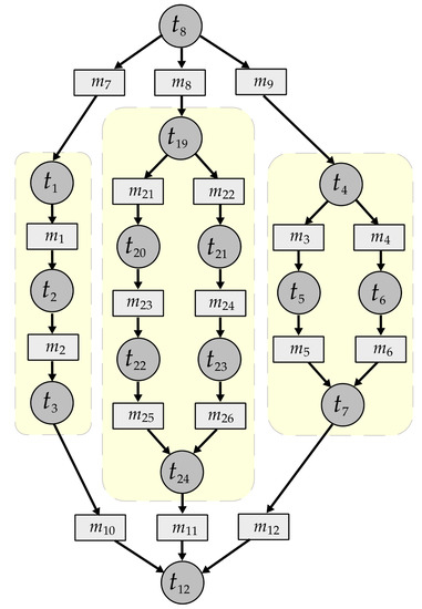
Figure 4.
Example of a two terminal series-parallel (TTSP) application graph.
Each computational task is associated with a worst-case execution time (WCET) for each PE of a heterogeneous hardware platform. Note that we write all execution times or delays in units of clock cycles of the global clock of the hardware platform, such that , too. For accuracy, the utilization of a computational task on a PE is defined in per mill as (). If a platform only contains homogeneous PEs, we simplify the equal WCET of each computational task on all tiles to and likewise the utilization of a task to . Furthermore, as a result of task scheduling in the system synthesis process (see Section 6), each computational task is assigned a start time of a time-triggered schedule on the PE it is executed on. During the system’s runtime, a computational task is executed without preemption in the time frame with .
Messages of application are the high-level entities that are exchanged between computational tasks for communication. Following [3], we assume that packets are the atomic entities transferred on the NoC. Depending on the amount of data in a message and the size of a data word of the hardware platform, a message is divided into several packets for the transfer on the NoC. For each message , the set of packets summarizes the decomposition of a message into packets. As packets are the atomic entities transferred on the NoC, we define for each resource of the NoC a processing delay that holds for all packets in the system for this particular resource. Note that this definition still enables the modeling of heterogeneous resources (NIs and routers) in the NoC. Similar to computational tasks, each packet of a message that is routed on a tree of resources of the NoC is assigned a start time in a time-triggered schedule on each resource .
Concerning the topology of applications graphs , as mentioned earlier, the paper at hand investigates a particular class of graphs, namely two terminal series-parallel (TTSP) application graphs [8]. Note that the graph depicted in Figure 4 is a TTSP application graph, as well as the yellow shaded sub-graphs. The TTSP application graphs capture the currently considerable sequential nature of control applications from the automotive domain as well as allow us to model the results of parallelizing these applications. The class of TTSP application graphs is defined recursively as follows:
Definition 1.
Two terminal series-parallel (TTSP) application graph (adapted from [8]):
- (i)
- An application graph with two computational tasks exchanging one message is a TTSP application graph.
- (ii)
- If the application graphs and are TTSP application graphs, so is the resulting application graph of the following two operations:
- (a)
- Two terminal parallel composition:Replace the source computational task of TTSP graph with the source computational task of TTSP graph and replace the sink computational task of with the sink computational task of .
- (b)
- Two terminal series composition:Replace the sink computational task of TTSP graph with the source computational task of TTSP graph .
The source computational task of a TTSP application graph is the computational task which is not connected to a message via an incoming edge, i.e., . Similar, the sink computational task of a TTSP application graph is the computational task with no outgoing edge to a message, i.e., , . As an example, in Figure 4, the source computational task is as well as the tasks and , if we look at the yellow shaded graphs individually. The sink computational task is , were again and are the sink computational tasks of the yellow shaded graphs. In Section 8.1 we describe how we generated the application graphs in our test instances and detail how we realized the merging of TTSP graphs.
4.3. Formal Problem Formulation
With the formal specifications presented in the previous two subsections, we provide a formal problem formulation of the synthesis problem during the design of time-triggered real-time systems.
The task of system synthesis is to find a valid implementation , consisting of a binding
the routing of all packets on resources of the NoC, and a feasible global time-triggered schedule for all computational tasks and packets of the application model.
A binding contains for each computational task of an application exactly one PE it is executed on. The routing contains the specific route of each packet of each message from its sending computational task to the receiving computational task on a set of connected resources of the NoC. Note that packets are not routed in the NoC if the sender of a message and the receiver of a message are bound on the same PE, i.e., . A time-triggered schedule contains the start times of all computational tasks on PEs and the start times of each packet on the resources of it route on the NoC. The time-triggered schedule has to resolve all resource access conflicts of shared resources and ensures that the deadlines of all applications are met (see Section 6).
In the following sections we will describe in detail how we solve the subproblems of binding, routing and scheduling in our coordinated system synthesis approach.
5. Answer Set Programming (ASP)—Binding & Routing
In the following section we briefly summarize how our coordinated synthesis approach leverages answer set programming (ASP) as logic solver (cf. Figure 2) to solve two sub-problems in system synthesis: the binding of computational tasks to PEs and routing of packets for inter-task communication on resources of the NoC. We refrain from introducing the ASP syntax as this would go beyond the scope of this paper. Instead, we point the interested reader to the relevant literature.
Answer set programming is a declarative problem solving approach with its origins in solving problems in the domain of knowledge representation and reasoning [11,12,13]. Among others, one of ASP’s distinguishing features is a rich and expressive, but yet simple modeling language, merged with state-of-the-art high performant solving techniques [16]. For system synthesis, ASP quite recently became an interesting alternative choice instead of Pseudo-Boolean satisfiability solving (PB-SAT) [14]. The authors showed that ASP scales better for densely connected architectures, such as NoC, compared to equivalent PB-SAT approaches. Here, the increased scalability is enabled by the possibility to express reachability within the modeling language of ASP directly, which is beneficial for multi-hop routing. These promising results encouraged us to favor ASP instead of PB-SAT solving to decide the routing and the binding in system synthesis.
Based on our formal system model (see Section 4), a problem instance for an answer set solver is formulated containing the information of the platform model and the send and receive dependencies of messages between computational tasks from the application model. A solution is then described in a problem encoding derived from [14], which captures relevant constraints of a feasible binding and routing: each computational task has to be bound to exactly one PE, the utilization of a PE should not exceed 100% and a route from sender to receiver should be acyclic. Furthermore, we include a necessary and sufficient condition to schedule two computational tasks on one resource non-preemptively [28]: Two computational tasks and with periods and and WCET and are schedulable if and only if
The benefit of adding this condition to the problem encoding of the answer set solver is that every pair of computational tasks can be scheduled on the same PE which therefore has not to be checked within the background theory. To the best to our knowledge, our work is the first one to include this constraint within the logic solver of an SMT-based synthesis approach.
5.1. Scheduling-Aware Binding & Routing Refinement
As mentioned before, in our coordinated SMT-based synthesis approach, we add additional lexicographical optimization goals to the answer set solver such that the background theory solver can decide schedulability within a shorter amount of time—a scheduling-aware binding and routing refinement. In Section 8 of this paper, we will show that despite adding the optimization goals introduces an additional overhead in terms of number of constraints and variables to the answer solver, this approach can significantly increase the scalability of symbolic system synthesis. Parts of the used encoding for lexicographical optimization goals can be found in [27]. Concerning the priorities of the optimization, we encode a load balancing strategy for the PEs of the platform with the highest priority. This is followed by minimizing the total number of routed messages on the platform and the total number of hops of all messages. With the lowest priority, we discourage sharing hardware resource between different applications since the complexity of the time-triggered scheduling increases considerably if hardware resources are shared by computational tasks or packets that do not belong to the same application.
5.2. Domain-Specific Heuristics in ASP
While ASP provides a rich modeling language together with highly performant yet general-purpose solving techniques, these general-purpose solving capabilities can further be boosted by utilizing domain-specific heuristics that are exploited at non-deterministic choice points [17]. Thus, the search heuristics already implemented in answer set solvers can be enriched with the knowledge of domain experts and potentially a better solution may be obtained within a shorter amount of time.
In the paper at hand, we focus on the heuristic presented in [27] which contains the most domain-specific knowledge and has also turned out to be most effective. In this heuristic, the answer set solver decides the binding of all computational tasks of one application before it decides the binding of any other computational tasks. Furthermore, the sending and the receiving computational task of a message should be bound to the same tile. If it is not possible to to bind all communicating tasks of one application to the same tile, e.g., due to load balancing computational load, we encode that next neighboring tiles should be preferred.
6. Time-Triggered Scheduling
We implemented time-triggered scheduling in our synthesis approach in order to resolve resource access conflicts on all resources of our hardware platform, namely all PEs for computation and the resources of the NoC for communication. Here, our time-triggered scheduling encoding [26,29] was originally based on refinements of [7,30] to fit different NoC-based architectures and includes improvements also presented in [31] in order to reduce scheduling constraints.
Note that several other work exists that mainly focuses solely on symbolic time-triggered scheduling without considering the overall system synthesis (binding, routing and scheduling). Some literature considers scheduling of messages only [32,33,34], whereas other work respects the more general problem of co-scheduling computational tasks and messages like in this paper [31,35,36,37].
In the following, we relinquish from presenting the full scheduling encoding for brevity. The interested reader may find more details in [29,31]. Overall, the constraints of the time-triggered scheduling ensure that a resource is at most used by one entity at the same time and precedence constraints among computational tasks and messages/packages are met. A feasible time-triggered schedule
contains periodic start times for all computational tasks and all packets contained the the system’s specification (cf. Section 4.2).
7. Coupling ASP and Background Theory
Given a binding and routing derived by the logic solver, a scheduling can be computed. However, in a first iteration of our SMT-based approach, two unfortunate observations can be made. First, deciding whether a binding and routing solution is schedulable takes considerable time, even if one uses our proposed coordinated approach. Second, early binding and routing solutions of the logic solver often cannot be scheduled.
A reason for the first observation is that in common approaches all computational tasks and packets are scheduled at once on the resources of the hardware platform. Thus, this results in a potentially large scheduling problem and usually long runtimes of the background theory in order to decide schedulability. Though, deciding feasibility of solution candidates in the background theory in a fast manner is a key ingredient for the performance of the whole synthesis approach. As a remedy, we address the first observation by introducing a hierarchical scheduling scheme suiting our system model based on modifications of the scheme introduced in [7] (see Figure 5).
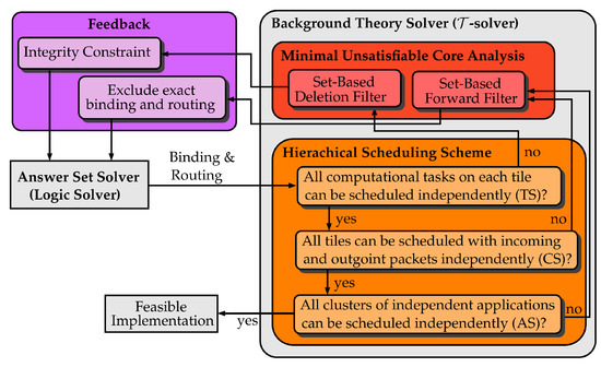
Figure 5.
Detailed overview of the flow within the coupling of the answer set solver and the background theory solver.
Instead of analyzing the whole system at once, we step through the stages of our scheme and decide on essential sub-problems:
- Schedule computational tasks on each tile independently (TS),
- Schedule computational tasks on each tile with the incoming and outgoing packets of the tile independently (CS),
- Schedule clusters of independent applications independently (AS).
Deciding the scheduling feasibility of the sub-problems usually takes considerably less time compared to deciding the complete system. Furthermore, if, e.g., already the computational tasks on one tile cannot be scheduled, scheduling the whole system is also not possible and further effort in stepping through the hierarchical scheduling scheme can be saved.
If all sub-problems of one stage are feasible, the problems of the subsequent stage in our hierarchical scheduling scheme are analyzed. Ultimately, if all sub-problems of the final stage can be solved, a feasible implementation is found. In contrast, if a sub-problem is infeasible, we are again in the situation of the second observation as stated above.
The second observation is addressed by providing accurate feedback from the background theory to the answer set solver as common in SMT-based approaches. Here, the feedback should at least prohibit that the exact same infeasible binding and routing is not proposed a second time. From related work, e.g., [6], we know that the scalability of symbolic system synthesis can further be significantly increased by deriving a minimal unsatisfiable core (MUC), i.e., a minimal reason why a schedule cannot be derived. Hence, if the MUC is propagated back to the answer set solver, often considerable amounts of infeasible design space can be pruned.
Once a sub-problem in the stage (TS) is infeasible, we apply a set-based deletion filter algorithm (see Algorithm 1) to deduce one MUC, similar to [7]. Let be the set of all computational tasks on one tile that form the infeasible set of constraints . In contrast to deletion filters known form the related work, e.g., [38], the set-based deletion filter requires only instead of iterations. Thus, deriving a MUC can be considerably faster since the number of tasks is noticeably lower than the number of constraints. Note that using the set-based deletion filter does not have any downsides in terms of expressiveness of the MUC since the logic solver does not relate to constraints that are used in the -solver. For example, in the case of scheduling computational tasks on tiles, the logic solver can only relate to entities of computational tasks.
Given a MUC of a problem in the (TS) stage in form of a set of computational tasks, an integrity constraint is propagated back to the answer set solver (see Figure 5). This constraints ensures that the same set of computational tasks within the MUC are not bound together on any tile of the hardware platform again. Thus, all bindings of the design space that contain this subset of an infeasible binding are effectively pruned.
| Algorithm 1 Set-based Deletion Filter for stage (TS). |
| Input: Unsatisfiable scheduling problem constraints C⊥ of stage (TS) and the corresponding set of tasks |
| Output: A minimal set of infeasible computational tasks |
| 1: C = C⊥ |
| 2: |
| 3: for t ∈ do |
| 4: if then |
| 5: |
| 6: |
| 7: end if |
| 8: end for |
| 9: return |
Regarding infeasible scheduling problems within stage (CS) and (AS), we found a forward filter [38] most suitable as it computes MUCs starting from smaller sets of constraints. Again, we modified the forward filter with a set-based approach to reduce the number of iterations to derive a MUC.
However, one main difference is that as sub-problems in the hierarchical scheduling stages (CS) and (AS) might also contain packets within the constraint set. Thus, the MUC also potentially contains packets as well as computational tasks. Without breaking symmetries, in our current setting the MUC is fed back to the answer set solver with the exact binding of computational tasks to tiles and the exact routing of messages. Since massively parallel architectures are often computation-centric and discourage a lot of communication by software design, the impact of not breaking symmetries can be considered negligible.
We note that the answer set solver is not restarted while the scheduling of implementation candidates is investigated within the background theory. Rather, the answer set solver is halted and “waits” for feedback. Thus, already learned knowledge in the answer set solver search algorithm, e.g., about optimally of solutions within the coordinated synthesis approach, is not lost.
8. Experimental Results
In the following section we present the experimental results showing the advantage of a coordinated SMT-based synthesis approach. We start by introducing our test instances and how they were generated and summarize our experimental setup. Furthermore, we discuss the experimental results of the classical non-coordinated synthesis approach, the coordinated synthesis approach and the coordinated synthesis approach that is enhanced with domain-specific heuristics.
8.1. Test Instances
The NoC-based hardware platforms of our test cases were regular 2D-meshes with such that a platform contained tiles in total. The resources of the platform (PEs, routers, …) were selected to be homogeneous. Thus, all computational tasks had the same WCET on all tiles and all packets were forwarded on the resources of the NoC within the same delay (). The delay of all packets was set to 10 cycles on all NIs and routers (). In order to convert time, e.g., computational time or periods of computational tasks and messages, into clock cycles of the hardware platform we used a common frequency of in available micro controllers for automotive or industrial applications [2].
The applications in our test cases are of synthetic nature and we do not rely on open-source benchmarks. There are two main reasons for this. First, massively parallel platforms cannot be computationally utilized in a meaningful way with control software that is running on current multi-core embedded systems. Thus, with multi-core software characteristics such as described in [39], the vast bulk of the hardware platform would be in idle state. As a remedy, our applications are oriented on the characteristics of state-of-the-art control software [39] (periods, amount of inter-task communication, …) but extrapolate towards higher system utilization.
Second, to the best to the authors’ knowledge, there is no published open-source benchmark for automotive control applications that respects the parameters described in [39] and allows us to systematically investigate scalability of our proposed methods. Also, note that we rather need a scheme that allows us to increase the computational utilization and total number of messages along with the increase in the size of our tiled mesh hardware architectures, rather than plain benchmark instances. In the following, we summarize the scheme we used to create synthetic test cases for a systematic evaluation of our approach. The source code of an implementation of this scheme together with the test cases that are investigated in this work can be obtained by mailing the paper’s last author.
In order to generate the applications to be executed on a given platform with tiles, we applied an algorithm including randomization in order to achieve diversity of the test cases within certain limits. As an important parameter in our generation scheme, the utilization factor defines the percentage the overall computational resources of the platform, i.e., all PEs, are utilized. For each of our test cases, we incrementally added randomized applications to the system until the total computational load of the system reached the desired overall computational load:
To generate the TTSP graph topology of one randomized application , we choose a simplified scheme based on five templates to create new TTSP graphs. Three of these templates are shown in Figure 4 as the yellow shaded TTSP graphs, whereas the two remaining templates are two TTSP graphs with three computational tasks in parallel, respectively, four parallel computational tasks in parallel. As a first step, one topology template was chosen randomly out of the set of five predefined template TTSP graphs. Then, each computational tasks that is not a sink or a source of the chosen TTSP template was replaced by a sub-graph that was at random either one of the TTSP templates or a single computational task. The resulting topology of the application graph is again a TTSP graph since it could also be created by the TTSP definition shown in Section 4.2. Note that the application graph in Figure 4 is one example which could result from the introduced two-step procedure.
For the parameters of each randomized application , we chose a random period from a set of non-harmonic periods common in the automotive domain [31,39]. The deadline of each application was constrained to its deadline, i.e., . The WCET of a computational task was implicitly defined by randomly selecting a utilization of a computational task . Regarding the messages exchanges between tasks, based on the task communication of real-world automotive applications [39], we chose for each message a random number of packets in . Since packets are the entities that are scheduled on the resource of the platforms NoC, the number of packets relating to a routed message influence considerably the number of constraints in the time-triggered scheduling problem in system synthesis (cf. Section 6).
Table 1 summarizes the average values of key characteristics of each of our testcase instance sets.

Table 1.
Overview instances: average numbers with standard deviation of 25 instances per system specification.
We label the sets of instances with N×N- using the dimension N of the 2D mesh of the NoC and the total computational utilization factor . Each set of instances consists of 25 randomly generated instances that where generated as described above. Table 1 reports the average total number of applications, the average total number of computational tasks, average total number of messages and average total number of packets of a test instance in the associated instance set along with the standard deviation. With increasing N and , we assume that the problem of synthesis becomes harder to solve as more tasks have to be bound, more messages to be routed on a larger NoC and overall more entities have to be scheduled. Note that for all the instances there exists at least one feasible synthesis. This has been checked independent of the results presented in the next section.
8.2. Experimental Setup
All experiments where performed on a workstation with a hexa-core Intel Xeon CPU E5-1650v2 at 3.50GHz running Ubuntu Linux as operating system. The total amount of accessible RAM in our experiments was limited to 62GB (note that the average RAM consumption over all synthesis runs within our experiments was 6.45GB.) using the tool benchexec [40].
To decide the binding and routing, we used clingo (version 5.2.2) [16] which combines the answer set solver clasp and the grounder gringo. As configuration of the answer set solver we used an automatic configuration (–configuration=auto) and also leveraged the parallel solving capabilities (–parallel-mode=6,split) where the search for answer sets is split onto the available six cores of our benchmarking workstation. In the coordinated approach, the optimization strategy was set to unsatisfiable core optimization strategy using (–opt-strategy=usc,4). Since this optimization strategy cannot be used together with domain-specific heuristics, we used a branch and bound optimization strategy (–opt-strategy=bb,2) when necessary. Both optimization strategies where selected based on the results of initial tests with the different optimization strategies that the used answer set solver has to offer.
For the coordinated approach, we further limited the optimization time for the answer set solver to 10 s. Note that this limited time is always additional for the optimization of a found initial solution for the binding and routing problem. After this time limit for optimization, the currently best solution is analyzed in the background theory. The answer set solver might also stop earlier, in this case it has proved that it found the best solution w.r.t. the prioritization of the optimization statements (cf. Section 5).
In the background theory, in order to test the limits of the classical uncoordinated approach to some extend independent of a background theory solver configuration, we made use of a portfolio solving approach. Here, any occurring scheduling problem is tried to be solved by the two SMT-solvers yices (version 2.5.4) [41] and Z3 (version 4.6.0) [42] in different configurations. Note that related work has shown that often SMT-solvers perform better in deciding the time-triggered scheduling problems considered in this paper compared to integer linear programming (ILP) approaches [31]. Once a scheduling problem is defined, different instances of the solver yices are started in parallel using the algorithms Floyd-Warshall (command line parameter –arith-solver=floyd-warshall) and the simplex algorithm (command line parameter –arith-solver=simplex) for the logic quantifier-free integer difference logic (QF_IDL). Furthermore, the results of [43] encouraged us to also start one instance of yices in quantifier-free linear integer arithmetic (QF_LIA) in default configuration. However, for our test instance, the linear integer arithmetic configuration does not show significant improvements compared to the integer difference logic of yices as suggested in [43]. Along with the different configuration of the yices solver, our portfolio approach also starts an instance of the Z3 solver in default configuration in logic QF_IDL.
Furthermore, we also try to decide arising scheduling problems faster by incorporating an UNSAT-hypothesis approach. Here, in every scheduling problem the constraints associated with scheduling computational tasks or messages on resources are incrementally added as long as the preceding problem was decided as feasible. The benefit of this iterative solving is that already a rather small (sub-)problem might be decided as infeasible within a shorter amount of time. Including this technique also resembles to some extent other approaches that try to decide on incomplete models (partial assignments on binding and routing variables), e.g., [9,10], but in our work this is more adapted to be consistent with the additions we made, e.g., the set-based deletion filter (cf. Section 7). Subsequently, if a problem is decided unsatisfiable in the iterations within the UNSAT-hypothesis, the unsatisfiable core extraction starts on a smaller problem instance. Similar to the portfolio solving approach for the background theory as described above, we invoke four different solver configuration for each scheduling problem in the UNSAT-hypothesis
Independent of which hypothesis was used to decide a scheduling problem instance, once any of the differently configured background theory solvers reached a point where it determined a scheduling problem as unsatisfiable or satisfiable, this result is used (including logging the respective runtime returned by the solver) and all other solver instances running in parallel are stopped.
Regarding the hierarchical scheduling scheme (cf. Section 7), at each stage we decide the feasibility of sub-problems iteratively. Once we found that a scheduling problem is not feasible, the associated MUC is extracted and immediately returned to the logic solver as explained in Section 7. Thus, no further sub-problems in a stage are tried to be solved once an infeasible solution was found.
Since our coordinated approach is non-deterministic, each instance is always run 5 times (what we also do for the classical approach). This non-determinism is due to the fact that we ultimately use the timer of the operation system to interrupt the lexicographical optimization in the answer set solver in the coordinated approach. Since the interruption by the timer might only jitter minimally, this is enough that the answer set solver might advance only a little bit in its solving process and other solutions are passed to the analysis in the background theory. By running each instance 5 times we gather statistics over the non-deterministic processes. The time limit for each run was always set to 3600 s in order to derive a feasible system synthesis.
8.3. Experimental Results
8.3.1. Results of Classical Approach without Coordination
Table 2 contains the results of the classical approach (columns “classical”) for the different instance sets as N×N- with the dimension of the 2D mesh of the NoC and the total computational utilization factor (see Section 8.1). The columns in Table 2 represent bins corresponding to the number of successfully solved instances out of 5 independent synthesis runs.
Table 2.
Overview of solved runs (up to five) for the 25 instances per instance set for the different synthesis approaches.
We observe that for “3 × 3-50-classic”, the platform where the 9 tiles are arranged in a 3 × 3 mesh grid with a total computational utilization of 50% of the platform, the classical synthesis is almost able to solve all except one instance of the 25 instances within at least one run of five runs per instance (based on the entry “1” in column “0/5” and column “classical”). However, there was no instance for which all five independent runs were solved. If the complexity of the synthesis problem is increased towards larger platforms and higher computational utilization, the classical approach is almost not able to solve any more instances. While the work at hand also includes refinements that should contribute to the scalability of the classical approach (which, best to our knowledge, are not considered in any other work on symbolic system synthesis), e.g., the Korst-constraint (cf. Equation (2)) in the answer set solver and the portfolio solving approach in the background theory, the classical approach is still not able to scale as desired.
For the runs of instances that reached the timeout, the bar chart in Figure 6 shows the average runtime distribution between the answer set solver (blue) and the background theory solver (red). Regarding the number of couplings where the background theory provided a feedback to restrict the search space of the answer set solver, this number was between 2 and 4. In the bar chart we observe that for the unfinished runs in the classical approach more than 90% of the time is spent on average in deciding whether a time-triggered schedule exists. Hence, a significant imbalance exists between the effort spend in the answer set solver and the background theory. A deeper evaluation also revealed that this time is almost exclusively spend in the scheduling stage where tiles are scheduled independently or the extraction of minimal unsatisfiable cores within tile schedules. This observation especially encouraged us to develop the load balancing scheme within the coordinated synthesis approach as discussed before (see Section 5).
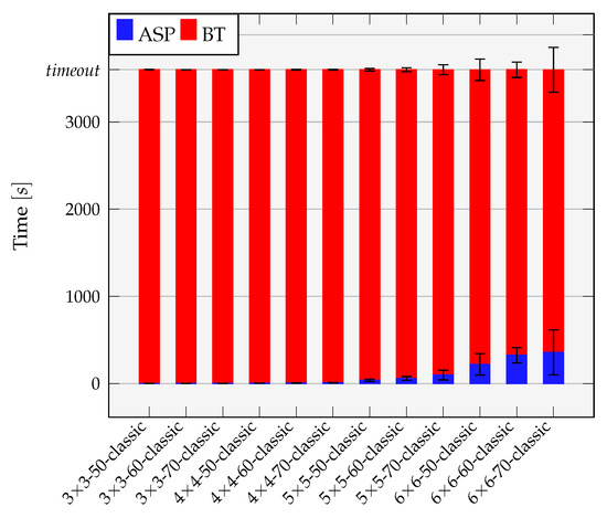
Figure 6.
Average runtime distribution between answer set solver (blue) and background theory solver (red) for the timeout runs in the classical approach. More than 90% of the total synthesis time is spent on average within the background theory until the timeout. The vertical error bars show the standard deviation.
8.3.2. Results of Coordinated Approach
Table 2 contains the number of solved runs for the different instances in the instance sets for the coordinated approach (columns “coord”). First of all, we compare the entries of the classical and the coordinated approach where none of the instances of an instance set is solved (“0/5” column). We see that up to the 5 × 5-70 instances the coordinated approach considerably more often is able to find at least one feasible synthesis out of five runs per instance than the classical approach.
Table 2 also indicates the limitations of the coordinated approach. Starting with the 5 × 5-70 instance set, considerably more instance cannot be synthesized within five independent runs of an instance. Ultimately, for the hardest instances of 6 × 6-70, only one run for one instance was solved. Despite this, by looking at the obtained results as a whole, the coordinated approach is still a considerable improvement regarding the applicability towards larger problem instances compared to the classical approach.
To one essential part, the increase in applicability of the coordinated approach is due to the load balancing objective in the coordinated approach as we conjecture that deciding schedulability of not fully utilized tiles can be considered as an easier task. Hence, in the background theory, the tile scheduling stage of the hierarchical scheduling scheme consumes significantly less time than in the classical approach. Furthermore, also the other optimization statements contribute to the improvement of the coordinated approach as these statements allow to decide scheduling faster within the independent application scheduling stage in the hierarchical scheduling scheme.
However, adding the necessary auxiliary variables and the optimization of the coordinated approach to the answer set solver comes with a non-negligible cost in terms of additional variables and constraints. Looking at our instances, the additional number of variables, which are reported by the answer set solver, increased between for the smaller instance up to for the largest instances. Similarly, the number of additional constraints increased between for the smallest instances, respectively, for the largest instances. As one numerical example, for the 6 × 6-70 instances and the classical approach, the average number of variables and constraints and the standart deviation was 821,999 ± 16,971 variables and 3,848,766 ± 303,098 constraints. In contrast, for the coordinated approach these values increase on average to 1,154,760 ± 35,410 variables and 5,198,396 ± 326,980 constraints.
Often, having more variables and constraints in the answer set solver can increase the time to derive a solution of the binding and routing sub-problem. Additionally, once an initial solution is found, the answer set solver spends up to to optimize this solution (or prove that the found initial one is the optimal solution). While for all the 3 × 3 mesh grid instances in the classical approach (note that more detailed data of the solved instances for the classical approach is not shown for the sake of brevity.) the total average time spend in the answer set solver in successful runs is less then , for the same instances it is around 20 s in the coordinated approach.
Figure 7 summarizes the average total times spent in the respective parts of the answer set solver and the background theory solver within the coordinated approach for the runs that finished successfully (note that the figure also contains the runtime for the enhancements with the DSH).
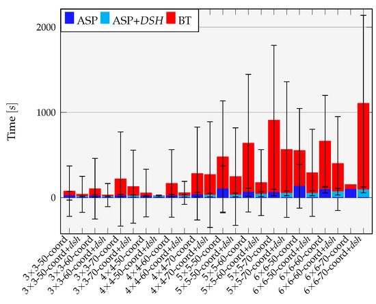
Figure 7.
Overview of the average distribution of runtimes of the successful runs using the coordinated approach and the coordinated+DSH approach for all instance sets. The vertical error bars show the standard deviation.
Regarding the number of couplings between logic solver and background theory, this number varies on average between 3 and 6. Note that the number of required couplings to find a feasible synthesis in all experiments of the work at hand is generally reduced. Here, the addition of the Korst-constraint (cf. Equation (2)) in the answer set solver, missing in previous approaches [26,27], already ensures that all pairwise computational task combinations on a tile are schedulable and potential pairwise scheduling conflicts are not encountered in the background theory anymore.
The changed distribution of efforts in Figure 7 between answer set solving and background theory solver compared to the classical approach becomes more prominent if one computes the quotient of averaged runtimes of the time spent in the background theory divided by the time spent in the answer set solver. This quotient is between 70 and 600 for all instances with 3 × 3 mesh grids in the classical approach, whereas the quotient is in the range 2–10 for all instances with any investigated mesh grid size in the coordinated synthesis approach. Thus, w.r.t. to the share of the overall solving time in the coordinated approach, considerable more effort is shifted to the answer set solver.
However, as already indicated earlier, starting with the 5 × 5-70 instances, also the coordinated approach reaches its limits. The Table 3, Table 4 and Table 5 capture three different categories of timeout runs of the coordinated approach.
Table 3.
Runtime distribution and number of timeout runs within the coordinated approach with timeout reached in the background theory (BT).
Table 4.
Runtime distribution and number of timeout runs within the coordinated approach with timeout reached in the answer set solver.
Table 5.
Number of runs that reached the memory limit within the background theory in the coordinated approach.
Here, the runs reaching the set timeout for a synthesis run can be divided into two categories: Table 3 shows selected data of runs of different instance sets where a synthesis run is dominated by the average time the coordinated approach spends within the background theory. This is similar to what we saw in the results for the classical approach but now we make this observation at considerable harder instance sets.
However, as a new observation, Table 4 shows average times of synthesis runs where the runtime until the timeout is mainly dominated by the answer set solver. In these cases, the answer set solver could not find a new binding and routing candidate in the meanwhile restricted search space after a few couplings with the background theory solver.
The final and third category is that for larger instances the background theory allocates memory reaching the overall synthesis memory limit and thus the synthesis run is canceled (cf. Table 5). Thereby, the memory limit is always reached in the last stage of the hierarchical scheduling scheme where the schedulability of independent app clusters is decided. However, in these cases there is always only one large application cluster resulting in scheduling problems spanning all hardware resources (PEs, NIs and routers) of the hardware platform. As a consequence, these scheduling problems are too memory intense to decide given our memory limit of 62 GB RAM.
All the results presented in Table 3, Table 4 and Table 5 are not desired as they limit the scalability of the coordinated synthesis approach, especially in the 6 × 6 mesh grid regime at higher utilization (cf. Table 2). Thus, we enhanced the coordinated synthesis approach by including domain-specific heuristics within the answer set solver. Again, the goal was to have “nicer” solutions proposed to the background theory which can be decided within reasonable time and without running into memory limitations. Furthermore, another goal was to reduce the occurring long solving times in the answer set solver as observed for some 6 × 6 mesh grid instances (cf. Table 4).
8.3.3. Results of Coordinated Approach with DSH
Table 2 (columns “DSH”) shows the respective number of solved instances for the coordinated+DSH approach. Furthermore, Figure 7 includes the average runtime distribution between the answer set solver and the background theory for solved runs of instances.
By comparing the solved instances between the coordinated approach with the coordinated+DSH approach we make two main observations. First and most obvious, the scaling by using DSH is significant better which is evident by looking at the “0/5” bin column starting at the 5 × 5-70 instance set. Second, by looking at the instances where more runs of an instance where solved (“5/5” and “4/5” bin), noticeable more runs of instances were solved in the regime of harder instance sets, i.e., those sets with 70% platform utilization. Thus, by using our domain knowledge encoded in the DSH, we are able to make the coordinated synthesis approach even more scalable and more robust (since more runs of instances are solved).
Regarding the time to derive a feasible system synthesis, by comparing the bars in Figure 7, the average time spend in the answer set solver and background theory solver is also always lower in the coordinated+DSH approach, and therefore is the average total synthesis time (with the exception of the single data point (single solved run) for 6 × 6-70-coord in Figure 7 which is neglected in our statement due to statistical relevance.)
Note that the answer set solver does not report any overhead in terms of additional variables or constraints if domain-specific heuristics are used within the coordinated approach. As described in [17], the additional formulation of the domain-specific heuristics are only used if non-deterministic choices have to be performed during the solving process and have no immediate contribution to the underlying complexity to the problem that needs to be solved.
While we also observed that the coordinated approach can spend a considerable amount of time within the answer set solver (see Table 4), this issue does not occur anymore if we use domain-specific heuristics together with the coordinated approach. Furthermore, not one synthesis run reaches the memory limit anymore.
Overall, our experiments show that the combined coordinated+DSH approach enriched with DSH considerably increases the scalability of the solely coordinated approach. Additionally, the average synthesis times are reduced. However, its limitations become more noticeable especially for the hardest instance set where almost half the instances in the 6 × 6-70 set could not be solved.
9. Concluding Remarks
Within our experimental section, we showed that previous related symbolic system synthesis approaches may lack applicability to scale beyond 3 × 3 tiled mesh architectures. In order to increase applicability towards larger and higher utilized architectures, we presented the coordinated synthesis approach. We realized the coordination by implementing a scheduling-aware binding and routing refinement in the logic solver, in our case an answer set solver. With this approach the logic solver is able to provide solution candidates to the background theory where schedulability can then be decided within a reasonable amount of time, which otherwise is not the case.
While the coordinated approach enhances the applicability of SMT-based system synthesis considerably, this approach reaches it limits around highly utilized 5 × 5-mesh architectures. We demonstrate how domain-specific knowledge encoded in domain-specific heuristics in the logic solver enables a further increase in scalability and robustness. Hence, we are able to solve significantly more runs from our instances sets up to around 6 × 6-mesh hardware architectures that are utilized on average at .
Author Contributions
Conceptualization, A.R. and C.H.; methodology, A.R.; software, A.R.; validation, A.R.; formal analysis, A.R.; investigation, A.R.; data curation, A.R.; writing—original draft preparation, A.R. and C.H.; writing—review and editing, A.R. and C.H.; visualization, A.R.; supervision, C.H.; project administration, C.H. All authors have read and agreed to the published version of the manuscript.
Funding
This work was partially funded by the German Science Foundation (DFG) under grant HA 4463/4-2.
Conflicts of Interest
The authors declare no conflict of interest.
References
- Gerstlauer, A.; Haubelt, C.; Pimentel, A.D.; Stefanov, T.P.; Gajski, D.D.; Teich, J. Electronic System-Level Synthesis Methodologies. IEEE Trans. Comput. Aided Des. Integr. Circuits Syst. 2009, 28, 1517–1530. [Google Scholar] [CrossRef]
- Infineon. AURIX 32-Bit TriCore TC2xx Product Specification. Available online: https://www.infineon.com/cms/en/product/microcontroller/32-bit-tricore-microcontroller/32-bit-tricore-aurix-tc2xx/ (accessed on 14 June 2022).
- Bjerregaard, T.; Mahadevan, S. A survey of research and practices of Network-on-chip. ACM Comput. Surv. 2006, 38, 1. [Google Scholar] [CrossRef]
- Hennessy, J.L.; Patterson, D.A. Computer Architecture—A Quantitative Approach, 5th ed.; Appendix F: Interconnection Networks; Morgan Kaufmann: Waltham, MA, USA, 2012. [Google Scholar]
- Reimann, F.; Glaß, M.; Haubelt, C.; Eberl, M.; Teich, J. Improving platform-based system synthesis by satisfiability modulo theories solving. In Proceedings of the 8th International Conference on Hardware/Software Codesign and System Synthesis, CODES+ISSS, Scottsdale, AZ, USA, 24–28 October 2010; pp. 135–144. [Google Scholar] [CrossRef]
- Reimann, F.; Lukasiewycz, M.; Glaß, M.; Haubelt, C.; Teich, J. Symbolic system synthesis in the presence of stringent real-time constraints. In Proceedings of the 48th Design Automation Conference, DAC, San Diego, CA, USA, 5–10 June 2011; pp. 393–398. [Google Scholar] [CrossRef]
- Lukasiewycz, M.; Chakraborty, S. Concurrent architecture and schedule optimization of time-triggered automotive systems. In Proceedings of the 10th International Conference on Hardware/Software Codesign and System Synthesis, CODES+ISSS, Tampere, Finland, 7–12 October 2012; pp. 383–392. [Google Scholar] [CrossRef]
- Valdes, J.; Tarjan, R.E.; Lawler, E.L. The recognition of Series Parallel digraphs. In Proceedings of the 11th Annual ACM Symposium on Theory of Computing, Atlanta, GE, USA, 30 April–2 May 1979; pp. 1–12. [Google Scholar] [CrossRef]
- Neubauer, K.; Wanko, P.; Schaub, T.; Haubelt, C. Enhancing symbolic system synthesis through ASPmT with partial assignment evaluation. In Proceedings of the Design, Automation & Test in Europe Conference & Exhibition, DATE, Lausanne, Switzerland, 27–31 March 2017; pp. 306–309. [Google Scholar] [CrossRef]
- Kumar, P.; Chokshi, D.B.; Thiele, L. A satisfiability approach to speed assignment for distributed real-time systems. In Proceedings of the Design, Automation and Test in Europe, DATE, Grenoble, France, 18–22 March 2013; pp. 749–754. [Google Scholar] [CrossRef]
- Baral, C. Knowledge Representation, Reasoning and Declarative Problem Solving; Cambridge University Press: Cambridge, UK, 2003. [Google Scholar] [CrossRef]
- Gelfond, M.; Kahl, Y. Knowledge Representation, Reasoning, and the Design of Intelligent Agents: The Answer-Set Programming Approach; Cambridge University Press: Cambridge, UK, 2014. [Google Scholar] [CrossRef]
- Gebser, M.; Kaminski, R.; Kaufmann, B.; Schaub, T. Answer Set Solving in Practice; Synthesis Lectures on Artificial Intelligence and Machine Learning; Morgan & Claypool Publishers: San Rafael, CA, USA, 2012. [Google Scholar] [CrossRef]
- Andres, B.; Gebser, M.; Schaub, T.; Haubelt, C.; Reimann, F.; Glaß, M. Symbolic System Synthesis Using Answer Set Programming. In Proceedings of the 12th International Conference on Logic Programming and Nonmonotonic Reasoning, LPNMR, Corunna, Spain, 15–19 September 2013; Volume 8148, pp. 79–91. [Google Scholar] [CrossRef]
- Barrett, C.W.; Sebastiani, R.; Seshia, S.A.; Tinelli, C. Satisfiability Modulo Theories. In Handbook of Satisfiability; IOS Press: Amsterdam, The Netherlands, 2009; Volume 185, pp. 825–885. [Google Scholar] [CrossRef]
- Gebser, M.; Kaufmann, B.; Schaub, T. Conflict-driven answer set solving: From theory to practice. Artif. Intell. 2012, 187, 52–89. [Google Scholar] [CrossRef]
- Gebser, M.; Kaufmann, B.; Romero, J.; Otero, R.; Schaub, T.; Wanko, P. Domain-Specific Heuristics in Answer Set Programming. In Proceedings of the Twenty-Seventh AAAI Conference on Artificial Intelligence, Bellevue, WA, USA, 14–18 July 2013. [Google Scholar]
- Lukasiewycz, M.; Streubühr, M.; Glaß, M.; Haubelt, C.; Teich, J. Combined system synthesis and communication architecture exploration for MPSoCs. In Proceedings of the Design, Automation and Test in Europe, DATE, Nice, France, 20–24 April 2009; pp. 472–477. [Google Scholar] [CrossRef]
- Nieuwenhuis, R.; Oliveras, A.; Tinelli, C. Solving SAT and SAT Modulo Theories: From an abstract Davis–Putnam–Logemann–Loveland procedure to DPLL(T). J. ACM 2006, 53, 937–977. [Google Scholar] [CrossRef]
- Satish, N.; Ravindran, K.; Keutzer, K. A decomposition-based constraint optimization approach for statically scheduling task graphs with communication delays to multiprocessors. In Proceedings of the Design, Automation and Test in Europe, DATE, Nice, France, 16–20 April 2007; pp. 57–62. [Google Scholar] [CrossRef]
- Liu, W.; Gu, Z.; Xu, J.; Wu, X.; Ye, Y. Satisfiability Modulo Graph Theory for Task Mapping and Scheduling on Multiprocessor Systems. IEEE Trans. Parallel Distrib. Syst. 2011, 22, 1382–1389. [Google Scholar] [CrossRef]
- Jackson, E.K.; Kang, E.; Dahlweid, M.; Seifert, D.; Santen, T. Components, platforms and possibilities: Towards generic automation for MDA. In Proceedings of the 10th International Conference on Embedded Software, EMSOFT, Scottsdale, AZ, USA, 24–29 October 2010; pp. 39–48. [Google Scholar] [CrossRef]
- Chakraborty, S.; Künzli, S.; Thiele, L. A General Framework for Analysing System Properties in Platform-Based Embedded System Designs. In Proceedings of the Design, Automation and Test in Europe, DATE, Munich, Germany, 3–7 March 2003; pp. 10190–10195. [Google Scholar] [CrossRef]
- Gebser, M.; Kaminski, R.; Kaufmann, B.; Ostrowski, M.; Schaub, T.; Wanko, P. Theory Solving Made Easy with Clingo 5. In Proceedings of the Technical Communications of the 32nd International Conference on Logic Programming, ICLP, New York, NY, USA, 16–21 October 2016; Volume 52, pp. 2:1–2:5. [Google Scholar] [CrossRef]
- Neubauer, K.; Beichler, B.; Haubelt, C. Exact Design Space Exploration Based on Consistent Approximations. Electronics 2020, 9, 1057. [Google Scholar] [CrossRef]
- Biewer, A.; Andres, B.; Gladigau, J.; Schaub, T.; Haubelt, C. A symbolic system synthesis approach for hard real-time systems based on coordinated SMT-solving. In Proceedings of the Design, Automation & Test in Europe, DATE, Grenoble, France, 9–13 March 2015; pp. 357–362. [Google Scholar]
- Andres, B.; Biewer, A.; Romero, J.; Haubelt, C.; Schaub, T. Improving Coordinated SMT-Based System Synthesis by Utilizing Domain-Specific Heuristics. In Proceedings of the 13th International Logic Programming and Nonmonotonic Reasoninh Conference, LPNMR, Lexington, KY, USA, 27–30 September 2015; pp. 55–68. [Google Scholar] [CrossRef]
- Korst, J.H.M.; Aarts, E.H.L.; Lenstra, J.K.; Wessels, J. Periodic Multiprocessor Scheduling. In Proceedings of the Parallel Architectures and Languages Europe, PARLE, Eindhoven, The Netherlands, 10–13 June 1991; pp. 166–178. [Google Scholar] [CrossRef]
- Biewer, A.; Munk, P.; Gladigau, J.; Haubelt, C. On the Influence of Hardware Design Options on Schedule Synthesis in Time-Triggered Real-Time Systems. In Proceedings of the Methoden und Beschreibungssprachen zur Modellierung und Verifikation von Schaltungen und Systemen, MBMV, Chemnitz, Germany, 3–4 March 2015; pp. 105–114. [Google Scholar]
- Lukasiewycz, M.; Schneider, R.; Goswami, D.; Chakraborty, S. Modular scheduling of distributed heterogeneous time-triggered automotive systems. In Proceedings of the 17th Asia and South Pacific Design Automation Conference, ASP-DAC, Sydney, Australia, 30 January–2 February 2012; pp. 665–670. [Google Scholar] [CrossRef]
- Minaeva, A.; Akesson, B.; Hanzálek, Z.; Dasari, D. Time-Triggered Co-Scheduling of Computation and Communication with Jitter Requirements. IEEE Trans. Comput. 2018, 67, 115–129. [Google Scholar] [CrossRef]
- Steiner, W. An Evaluation of SMT-Based Schedule Synthesis for Time-Triggered Multi-hop Networks. In Proceedings of the 31st IEEE Real-Time Systems Symposium, RTSS, San Diego, CA, USA, 30 November–3 December 2010; pp. 375–384. [Google Scholar] [CrossRef]
- Steiner, W. Synthesis of Static Communication Schedules for Mixed-Criticality Systems. In Proceedings of the 14th IEEE International Symposium on Object/Component/Service-Oriented Real-Time Distributed Computing Workshops, ISORC Workshops, Newport Beach, CA, USA, 28–31 March 2011; pp. 11–18. [Google Scholar] [CrossRef]
- Huang, J.; Blech, J.O.; Raabe, A.; Buckl, C.; Knoll, A.C. Static scheduling of a Time-Triggered Network-on-Chip based on SMT solving. In Proceedings of the Design, Automation & Test in Europe, DATE, Dresden Germany, 12–16 March 2012; pp. 509–514. [Google Scholar] [CrossRef]
- Craciunas, S.S.; Oliver, R.S. SMT-based Task- and Network-level Static Schedule Generation for Time-Triggered Networked Systems. In Proceedings of the 22nd International Conference on Real-Time Networks and Systems, RTNS, Versailles, France, 8–10 October 2014; p. 45. [Google Scholar] [CrossRef]
- Zhang, L.; Goswami, D.; Schneider, R.; Chakraborty, S. Task- and network-level schedule co-synthesis of Ethernet-based time-triggered systems. In Proceedings of the 19th Asia and South Pacific Design Automation Conference, ASP-DAC, Singapore, 20–23 January 2014; pp. 119–124. [Google Scholar] [CrossRef]
- Schweissguth, E.B.; Danielis, P.; Timmermann, D.; Parzyjegla, H.; Mühl, G. ILP-based joint routing and scheduling for time-triggered networks. In Proceedings of the 25th International Conference on Real-Time Networks and Systems, RTNS, Grenoble, France, 4–6 October 2017; pp. 8–17. [Google Scholar] [CrossRef]
- Ostrowski, M.; Schaub, T. ASP modulo CSP: The clingcon system. Theory Pract. Log. Program. 2012, 12, 485–503. [Google Scholar] [CrossRef][Green Version]
- Kramer, S.; Ziegenbein, D.; Hamann, A. Real world automotive benchmarks for free. In Proceedings of the 6th International Workshop on Analysis Tools and Methodologies for Embedded and Real-time Systems, WATERS, Lund, Sweden, 7 July 2015. [Google Scholar]
- Beyer, D. Reliable and Reproducible Competition Results with BenchExec and Witnesses (Report on SV-COMP 2016). In Proceedings of the 22nd International Conference Tools and Algorithms for the Construction and Analysis of Systems, TACAS, Eindhoven, The Netherlands, 2–8 April 2016; Volume 9636, pp. 887–904. [Google Scholar] [CrossRef]
- Dutertre, B. Yices 2.2. In Proceedings of the 26th International Conference on Computer Aided Verification, CAV, Vienna, Austria, 18–22 July 2014; Volume 8559, pp. 737–744. [Google Scholar] [CrossRef]
- De Moura, L.M.; Bjørner, N. Z3: An Efficient SMT Solver. In Proceedings of the 14th International Conference on Tools and Algorithms for the Construction and Analysis of Systems, TACAS, Munich, Germany, 29 March–6 April 2008; Volume 4963, pp. 337–340. [Google Scholar] [CrossRef]
- Pozo, F.; Rodríguez-Navas, G.; Hansson, H.; Steiner, W. SMT-based synthesis of TTEthernet schedules: A performance study. In Proceedings of the 10th IEEE International Symposium on Industrial Embedded Systems, SIES, Siegen, Germany, 8–10 June 2015; pp. 162–165. [Google Scholar] [CrossRef]


Publisher’s Note: MDPI stays neutral with regard to jurisdictional claims in published maps and institutional affiliations. |
© 2022 by the authors. Licensee MDPI, Basel, Switzerland. This article is an open access article distributed under the terms and conditions of the Creative Commons Attribution (CC BY) license (https://creativecommons.org/licenses/by/4.0/).