Ground Pedestrian and Vehicle Detections Using Imaging Environment Perception Mechanisms and Deep Learning Networks

Abstract

In order to build a robust network for the unmanned aerial vehicle (UAV)-based ground pedestrian and vehicle detection with a small number of training datasets but strong luminance environment adaptability, a system that considers both environment perception computation and a lightweight deep learning network is proposed. Because the visible light camera is sensitive to complex environmental lights, the following computational steps are designed: First, entropy-based imaging luminance descriptors are calculated; after image data are transformed from RGB to Lab color space, the mean-subtracted and contrast-normalized (MSCN) values are computed for each component in Lab color space, and then information entropies were estimated using MSCN values. Second, environment perception was performed. A support vector machine (SVM) was trained to classify the imaging luminance into excellent, ordinary, and severe luminance degrees. The inputs of SVM are information entropies; the output is the imaging luminance degree. Finally, six improved Yolov3-tiny networks were designed for robust ground pedestrian and vehicle detections. Extensive experiment results indicate that our mean average precisions (MAPs) of pedestrian and vehicle detections can be better than ~80% and ~94%, respectively, which overmatch the corresponding results of ordinary Yolov3-tiny and some other deep learning networks.

1. Introduction

Intelligent surveillance [1] is one of key construction targets of smart cities. Intelligent surveillance can realize pedestrian behavior analysis [2], traffic flow monitoring, abnormal information forecasting, and early dangerous state warning [3], etc. Many systems, such as ground or airborne surveillance terminals, can be considered for intelligent surveillance applications. Compared with the ground system, airborne surveillance equipment uses unmanned aerial vehicles (UAVs) to collect images with large view fields and view angles, which can provide convenient applications for ground target detection [4]. Currently, visible light cameras are commonly used for UAV surveillance. A visible light camera can capture vivid imaging data for observation and analysis; however, the complex environment light will always degrade its imaging effect [5] dramatically. For example, when long-endurance UAVs are used for information collection, it will experience problems with respect to changes in light intensity and direction, the scale and posture differences of the ground target, and the partial occlusion of complex scenes. Thus, designing a robust and highly efficient ground target detection method is a requirement that the municipal administration department is considering.

Three kinds of techniques have been developed to improve the imaging effect and computational robustness of visible light camera-based systems. The first method uses an optic filter [6] to constrain the negative influence of environmental light. The drawback of this method is observed when the imaging output is not adequate for observation because too many details in typical spectral bands are filtered. The second technique utilizes an image enhancement algorithm [7] to improve imaging quality. The shortcoming of this technique consists in its poor computational robustness for complex environment changes. The third measurement employs neural networks (especially the deep learning network [8]) to strengthen target detection effects. Unfortunately, the requirement of a large amount of training data and its slow training processing always limit its application in practical tasks. Recently, the technique of using lightweight deep learning networks [9] can solve this problem to some extent; moreover, much attention is currently directed toward designing this type of network.

Deep learning network has met its great success in recent years. Regarding the target detection task, in general, deep learning network can be classified into the one-stage method and two-stage approach [10]. The one-stage method uses regression analysis to detect targets. This method omits the generation procedure of candidate regions and gets target classification and position information directly. On the other hand, the two-stage approach considers selective searching or edge boxes to obtain the possible target-contained region proposal; then, it estimates the target region by using candidate region classification and position regression. The representative networks and their computational flow charts are illustrated in

Table 1. The representative methods of deep learning network for target detection.

Network Type	Representative Network
One-stage method	You only look once (Yolo) series [11,12], single shot multibox detector (SSD) series [13,14], RetinaNet [15], CornerNet [16], CenterNet [17], and EfficientDet [18].
Two-stage approach	Region-based convolutional neural network (R-CNN) [19], spatial pyramid pooling network (SPP-Net) [20], Fast R-CNN [21], Faster R-CNN [22], Mask R-CNN [23], Cascade R-CNN [24], and TridentNet [25].

and Figure 1. Another classification method of deep learning technique includes anchor-based and anchor-free methods. The anchor boxes are a type of multi-scale descriptor that can mark potential regions of target. For example, most methods listed in Table 1 belong to the anchor-based method, with the exception of CornerNet.

Applying target detection in outdoor environment will always be confronted with a series of problems. In addition to the complex environment illumination, atmosphere phenomenon, and different photography methods, the limited computational resource and training data will also induce problems for the process of algorithm design. When the target size is small, e.g., the aerial application, the large size of the convolution function, unideal distribution of training dataset, weak generalization ability of network model, improper setting of the anchor box, and suboptimal design of intersection over union will influence the performance of target detection. To conquer these difficulties, lightweight deep learning technique can be used. A lightweight network pursues highly efficient network design methods; the high-performance computation of convolution is also used to reduce the complexity of the network’s structure. The typical lightweight network includes MobileNet [26], SqueezeNet [27], or ShuffleNet [28], etc. Another solution for small numbers of training datasets relative to deep learning networks is using transfer learning. Transfer learning considers the accumulated knowledge and transfer mechanism to construct a network; however, a basic trained deep learning network is still needed.

In this paper, a ground pedestrian and vehicle detection method that considers both imaging environment perception and deep learning network is proposed for UAV applications. Regarding the environment perception method, after image data were transformed from RGB to Lab color space [29], the mean subtracted and contrast normalized (MSCN) values [30] were computed for each Lab component; then, the information entropy indices [31] were estimated using MSCN values. The support vector machine (SVM) [32] is used to classify imaging luminance into three degrees. Clearly, environment perception can realize image luminance classification for the following target detection according to imaging quality. As for ground pedestrian and vehicle detections, six improved Yolov3-tiny networks [33] with their typical network structures were designed. Each network has better detection performances for ground pedestrian and vehicle identification under its respective environment luminance scope.

Yolov3-tiny can realize a fast network calculation by simplifying the structure of Yolov3. Because its feature extraction structure has a few convolution layers and pooling layers, the extracted features are not rich enough and the average accuracy and recall rate are also not ideal. As for the application of UAV ground object recognition, the sizes and length–width ratios of vehicles and pedestrians in ground image are not fixed, and missing and false detections can be found easily when the target is far away from camera or changes its shape significantly. Therefore, balancing detection accuracy and network structure is a difficult problem in this research field [34,35]. In this paper, by subdividing the vehicles and pedestrians by their sizes as well as the environmental light by its intensity, a series of improved Yolov3-tiny networks was proposed, and then an efficient ground object detection method can be realized.

The main contributions of this paper include the following.

(1)

A ground pedestrian and vehicle detection method, which considers both luminance evaluation-based environment perception and improved one-stage lightweight deep learning network, is developed.

(2)

The MSCN values, information entropy indices, and SVM classification are considered for implementing imaging luminance estimation.

(3)

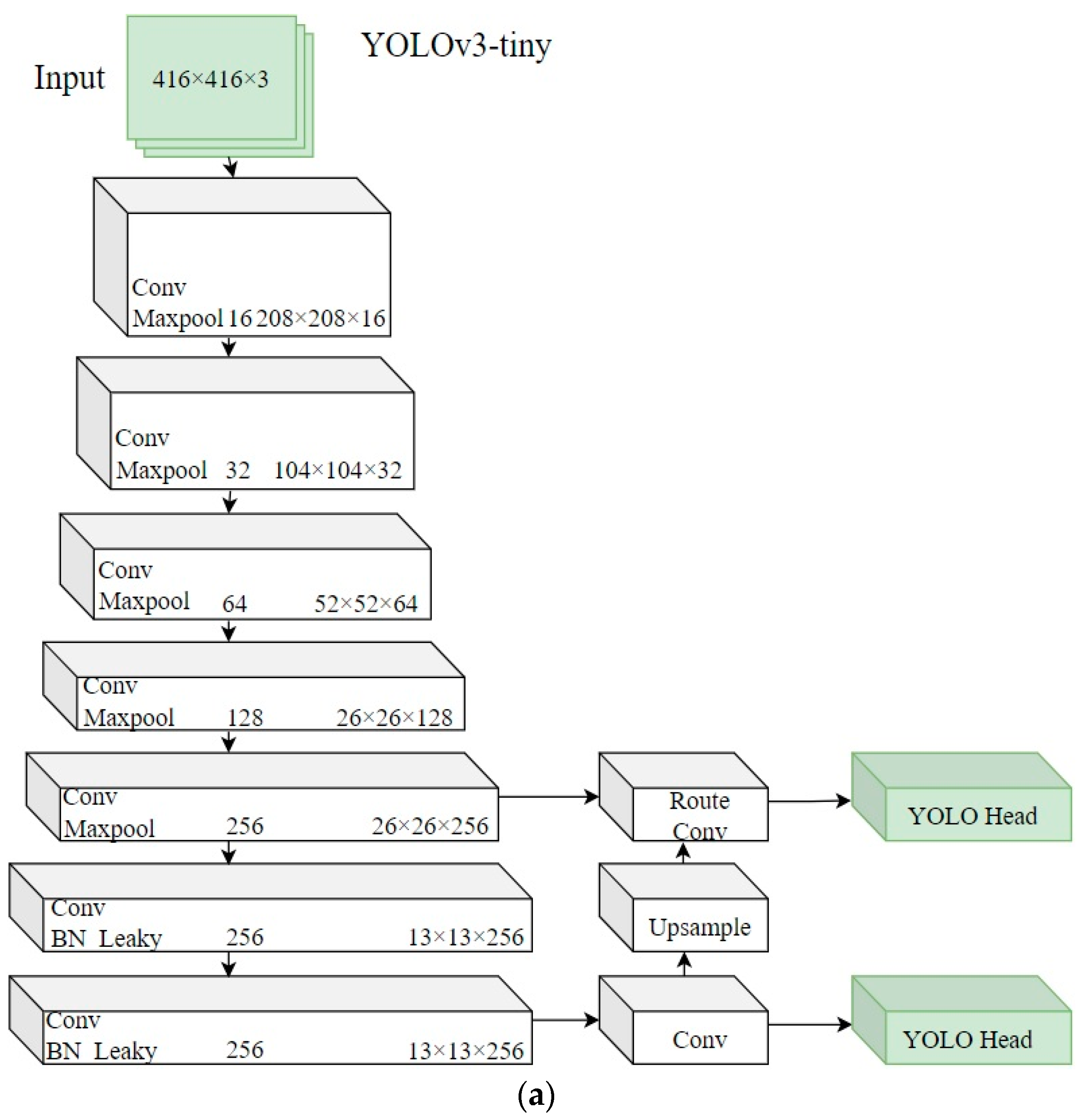
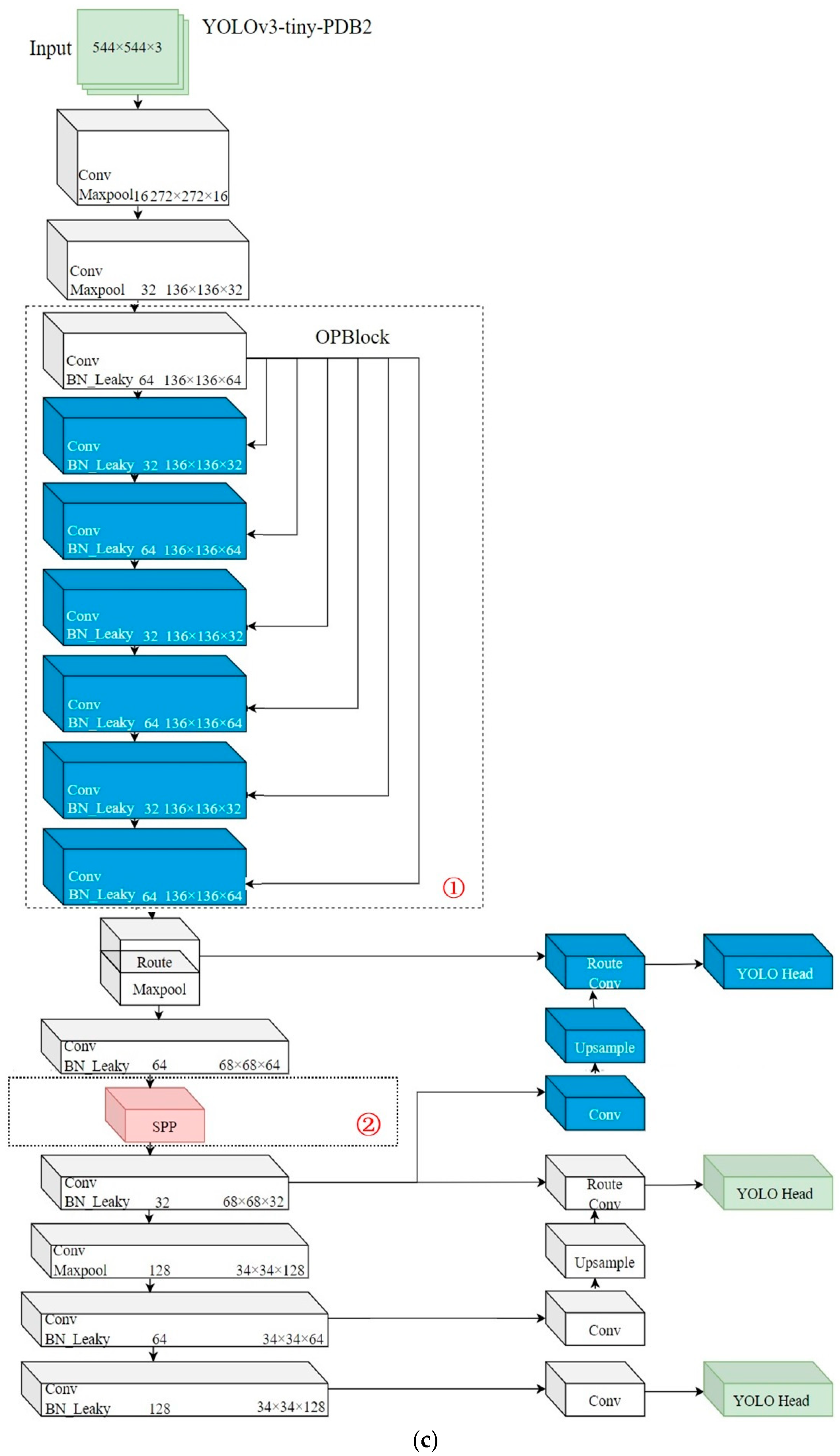
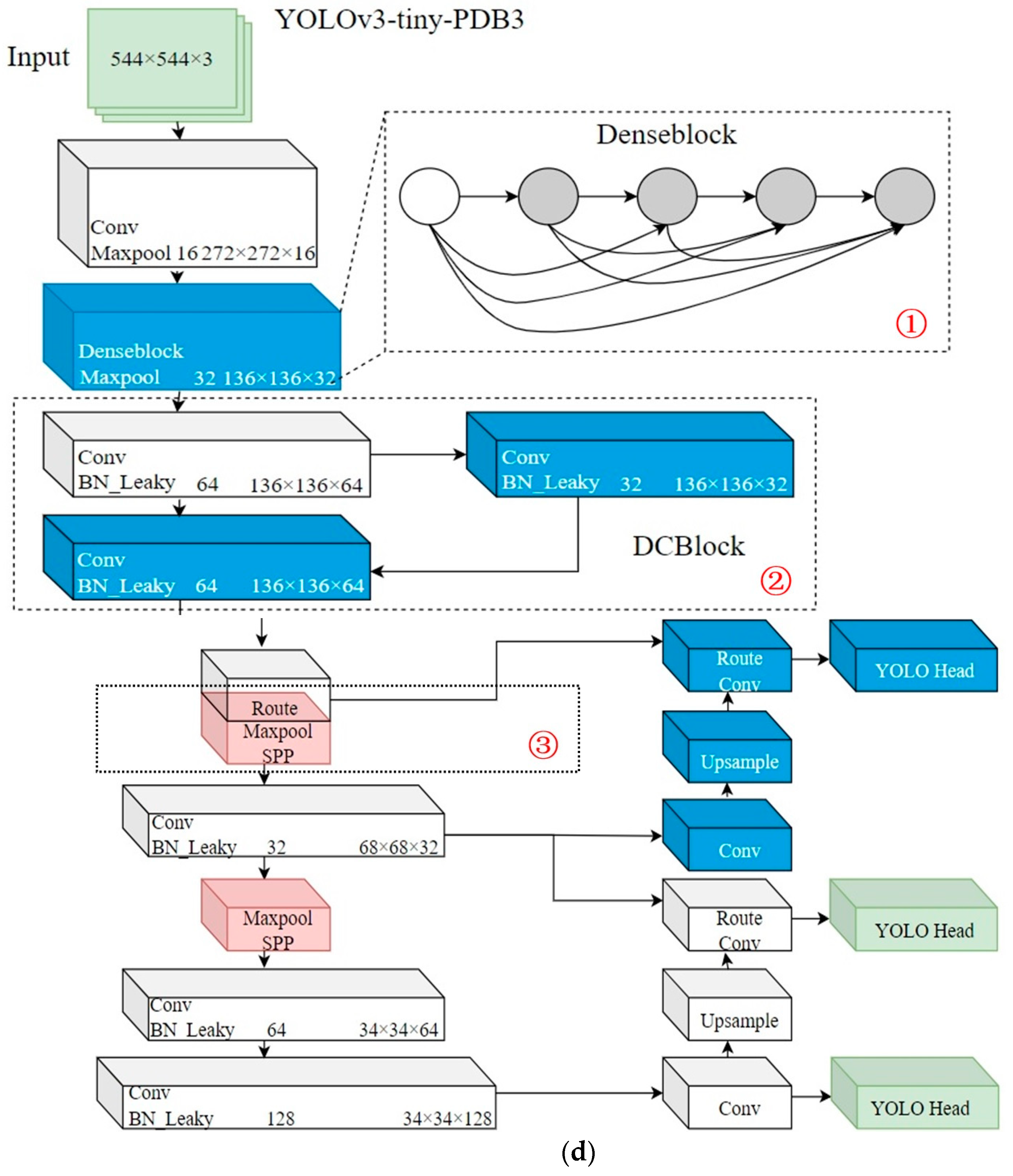
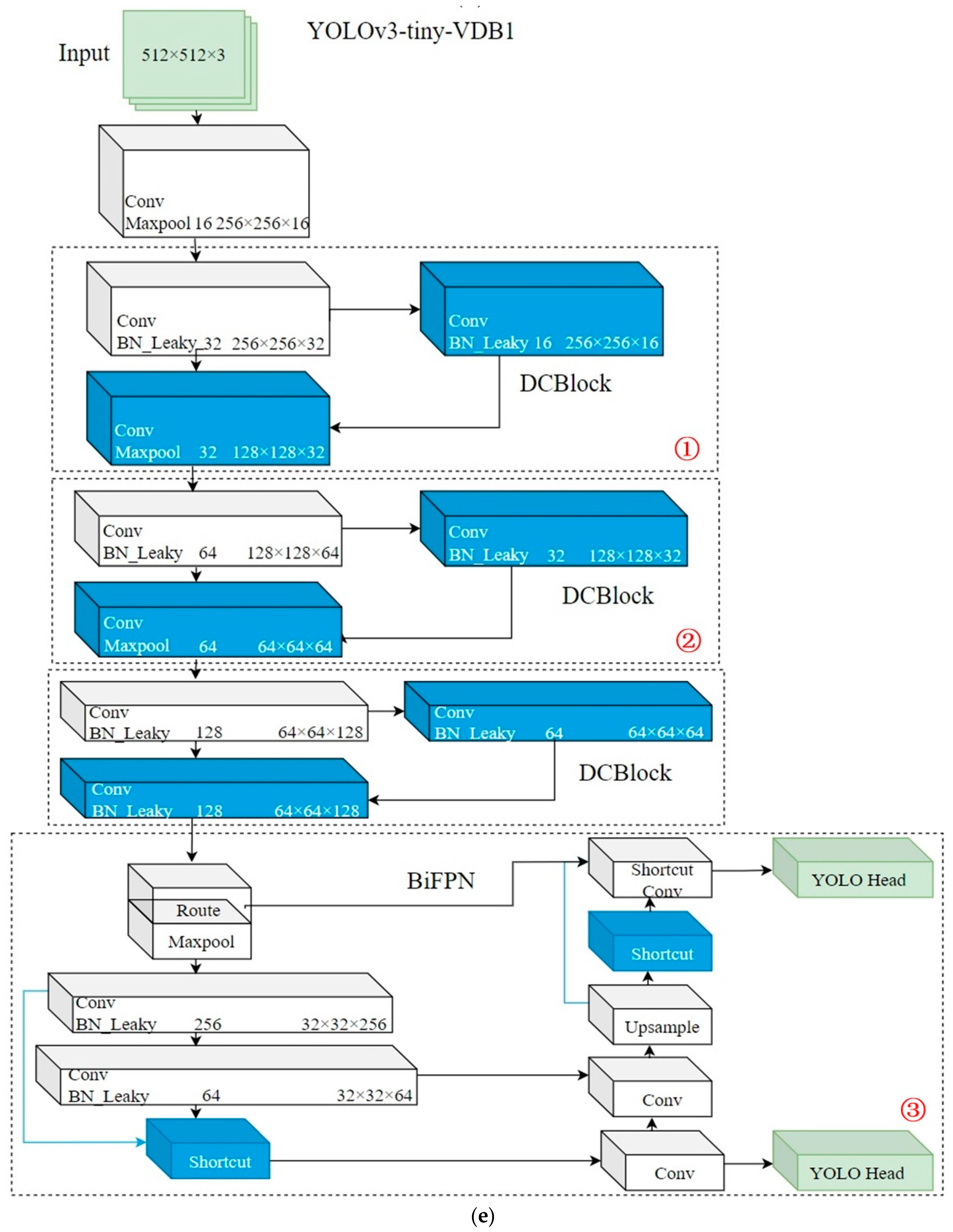
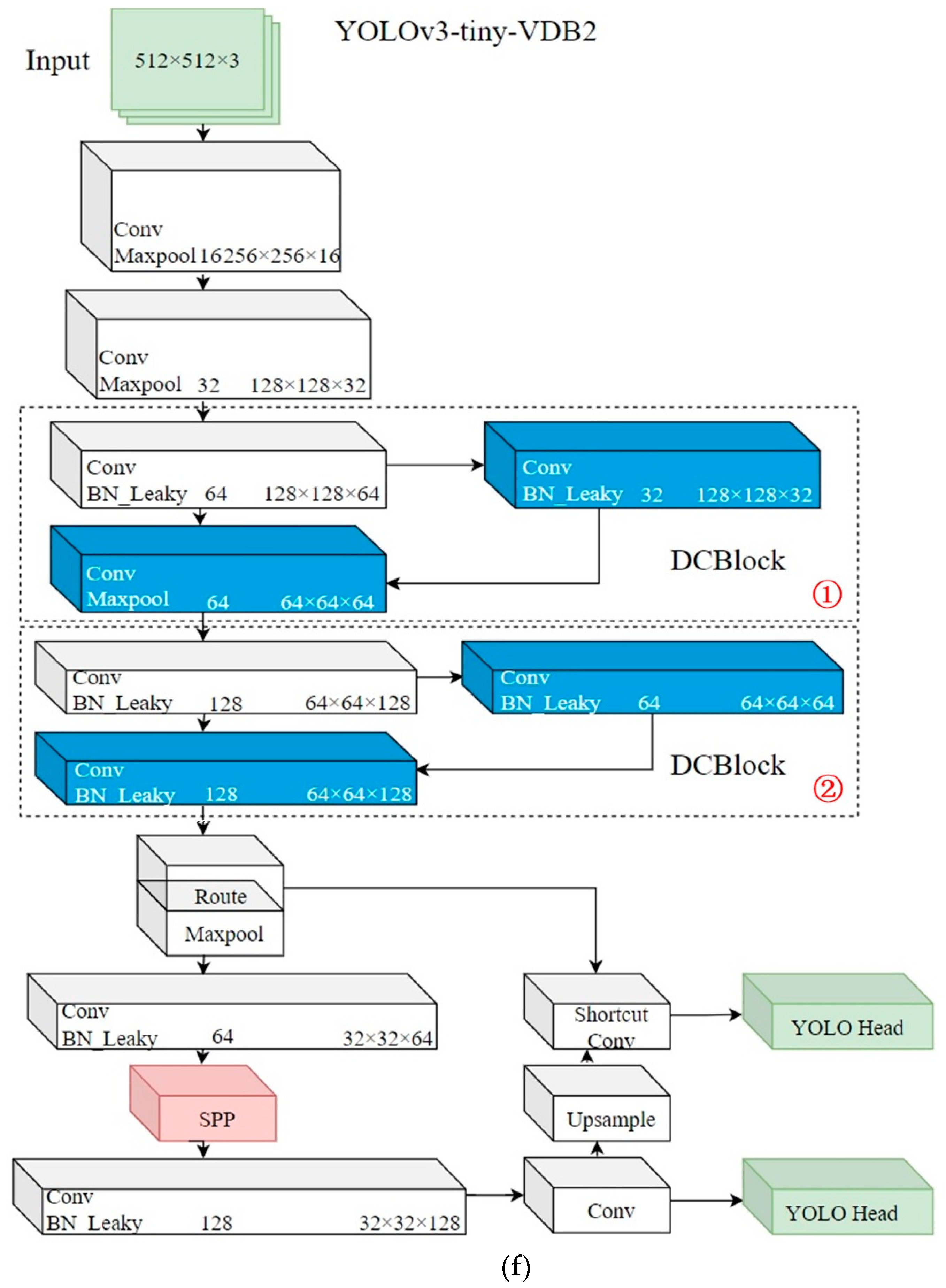
DCBlock, OPBlock, and Denseblock are designed or used in Yolov3-tiny to realize a robust pedestrian and vehicle detection under complex imaging luminance.

In the following sections, first, the proposed algorithm will be presented in detail. Second, the data source, comparison and evaluation experiments, and performance discussions will be illustrated. Finally, a conclusion is provided.

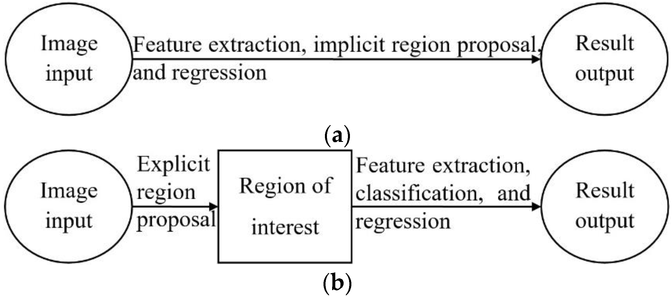
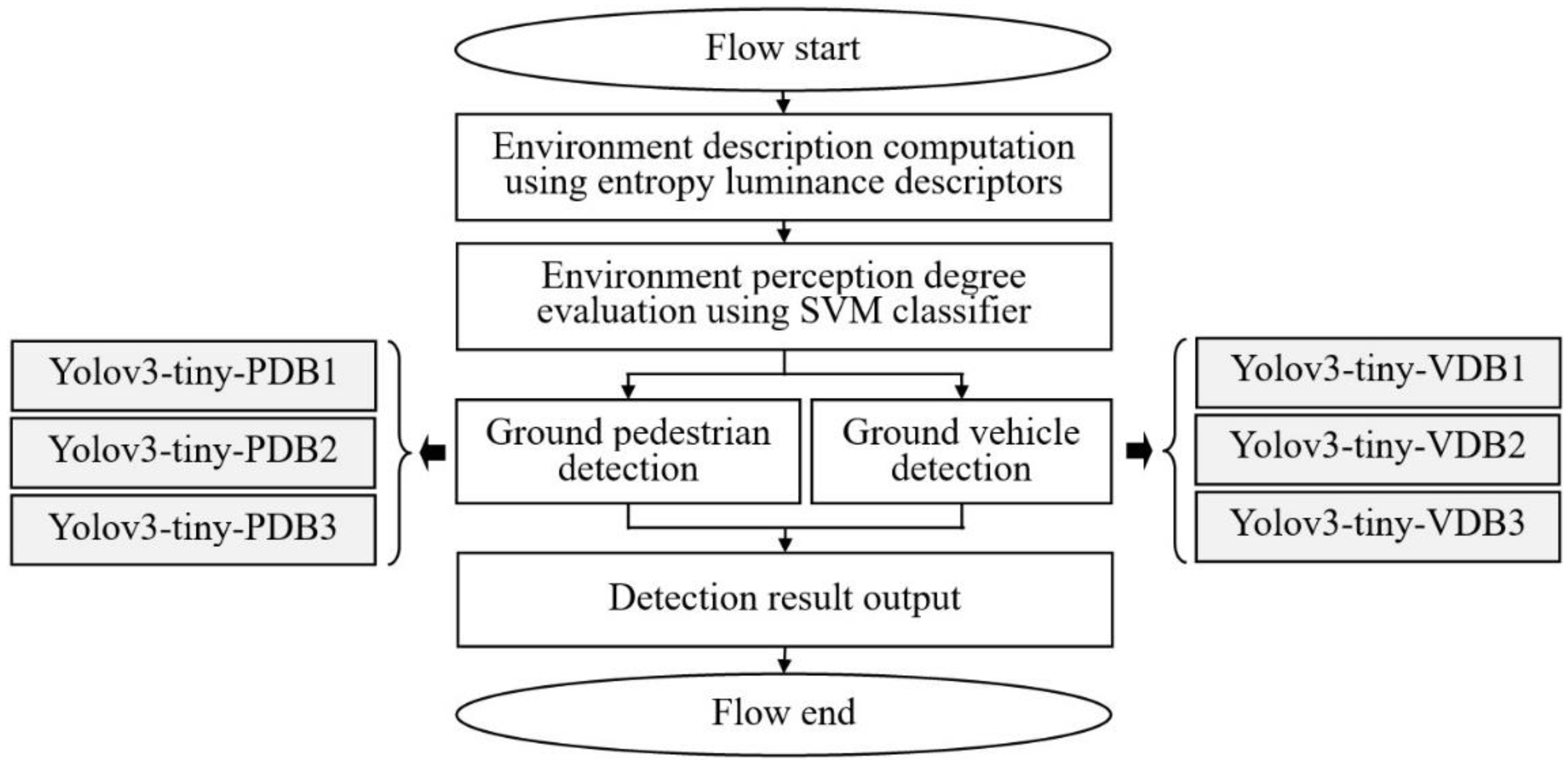
2. Proposed Algorithm

Figure 2 presents the proposed computational flow chart of our ground pedestrian and vehicle detection algorithm. From Figure 2, both the entropy-based luminance descriptor and SVM classifier are used for imaging environment perception; six improved Yolov3-tiny networks are used for ground pedestrian and vehicle detections. In Figure 2, Yolov3-tiny-PDB1, Yolov3-tiny-PDB2, and Yolov3-tiny-PDB3 were employed to detect ground pedestrians when imaging luminance is excellent, ordinary, and severe, respectively. Yolov3-tiny-VDB1, Yolov3-tiny-VDB2, and Yolov3-tiny-VDB3 were used to detect ground vehicle when imaging luminance is excellent, ordinary, and severe. Excellent imaging luminance means that the environment’s light intensity is ~≥1500 lx; ordinary imaging luminance means that the environment’s light intensity is ~≥300 lx and ~<1500 lx; severe imaging luminance indicates that the environment’s light intensity is ~≥50 lx and ~<300 lx.

2.1. The Color Space Transform

When our system captures an image, the color space transformation transition from RGB to Lab color space. Lab color space was authenticated by the International Commission on Illumination. It was initially invented to describe illumination and color more accurately. In Lab color space, component L is a correlate of lightness, component a represents the degree of redness versus greenness, and component b indicates the degree of yellow color versus blue color. Compared with RGB color space, color expressions in Lab color space are closer to the cognition effect of people [36], i.e., it is perceptual uniform; as a result, the imaging quality evaluation in Lab color space will have better performance in luminance evaluation. Luminance can reflect the luminous intensity or light response intensity of the matter. When it is associated with an imaging application, luminance estimation should be connected with both objective radiation intensity and the subjective perception degree relative to people; after all, people are the designers or users of imaging system or image processing algorithm.

2.2. The Environment Perception Computation

After color space transformation, first, the MSCN values were computed. MSCN [30] is a normalized illumination that can enhance the distribution character of the original data [37]. For example, after MSCN computation, the processed data will have strong distribution performances of standard Gaussian distribution. Clearly, Gaussian distribution has good performances in data analysis and computation. Equations (1)–(3) present the computational method of MSCN values; clearly, they also belong to data standardization processing [38] from a data preprocessing point of view. MSCN can reduce content influences from neighboring pixels in the image; this also indicates the following: As a kind of image quality evaluation metric, MSCN has better robustness in terms of restraint from disturbances in image content [39]. Second, information entropy indices are computed. Information entropy [31] represents the amount of information of typical distribution. It also can be comprehended as the average amount of information after redundancy exclusion. Equation (4) is its computational method. Clearly, since MSCN values can reflect statistical features of input image and the entropy can also disclose the image structure feature; the sequential computations of MSCN and information entropy can represent image luminance to some extent. Third, SVM is used for imaging luminance classification. It is well known that SVM can obtain good classification accuracy only with a small amount of training data. In addition, it possesses fast processing speed; therefore, a three-input and one-output SVM is utilized in this study:

$${I^{\prime }}_X\left(i,j\right)=\frac{I_X\left(i,j\right)-{\mu }_X\left(i,j\right)}{{\sigma }_X\left(i,j\right)+C}$$

(1)

$${\mu }_X\left(i,j\right)={\displaystyle \sum _{k=-K}^K{\displaystyle \sum _{l=-L}^L{w}_{k,l}{I}_X\left(i+k,j+l\right)}}$$

(2)

$${\sigma }_X\left(i,j\right)=\sqrt{{\displaystyle \sum _{k=-K}^K{\displaystyle \sum _{l=-L}^L{w}_{k,l}{\left[I_X\left(i+k,j+l\right)-{\mu }_X\left(i,j\right)\right]}^2}}}$$

(3)

$$H_X=-{\displaystyle \sum _{m=0}^{255}{P}_X\left(m\right){\log }_2{P}_X\left(m\right)}$$

(4)

where I_X(i, j) is the imaging intensity of the X component of the Lab color space in position (i, j), i = 1, 2, …, M, j = 1, 2, …, N; M and N are the height and weight of the input image; I’_X(i, j) is the MSCN estimation result of I_X(i, j); μ_X(i, j) is the mean value of I_X(i, j); σ_X(i, j) is the standard deviation value of I_X(i, j); C is a constant, C = 1.0, in this paper; X ∈ {L, a, b}; w_{k, l} is a Gaussian filter; k and l are the sizes of discrete Gaussian filter, k = −K, …, K, l = −L, …, L, K = 2, L = 2 in this paper; H_X is the information entropy of the X component; P_X(m) is the histogram value of I’_X(i, j) in gray intensity m.

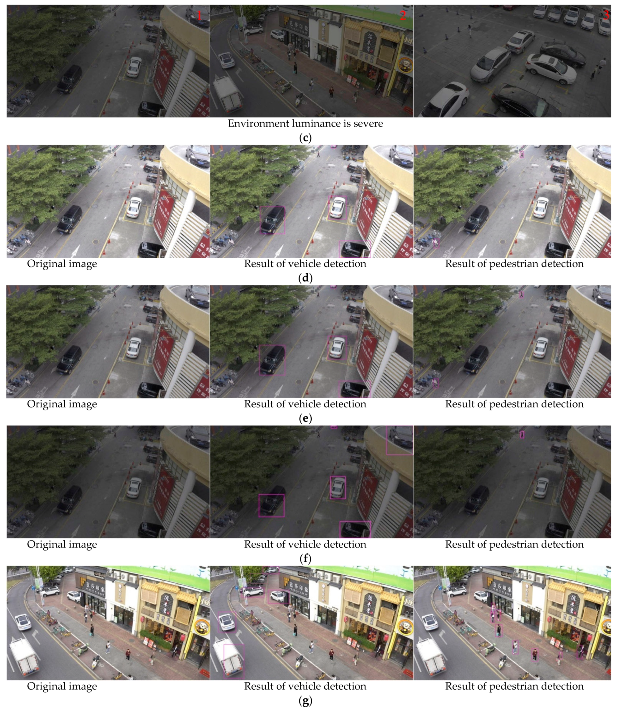
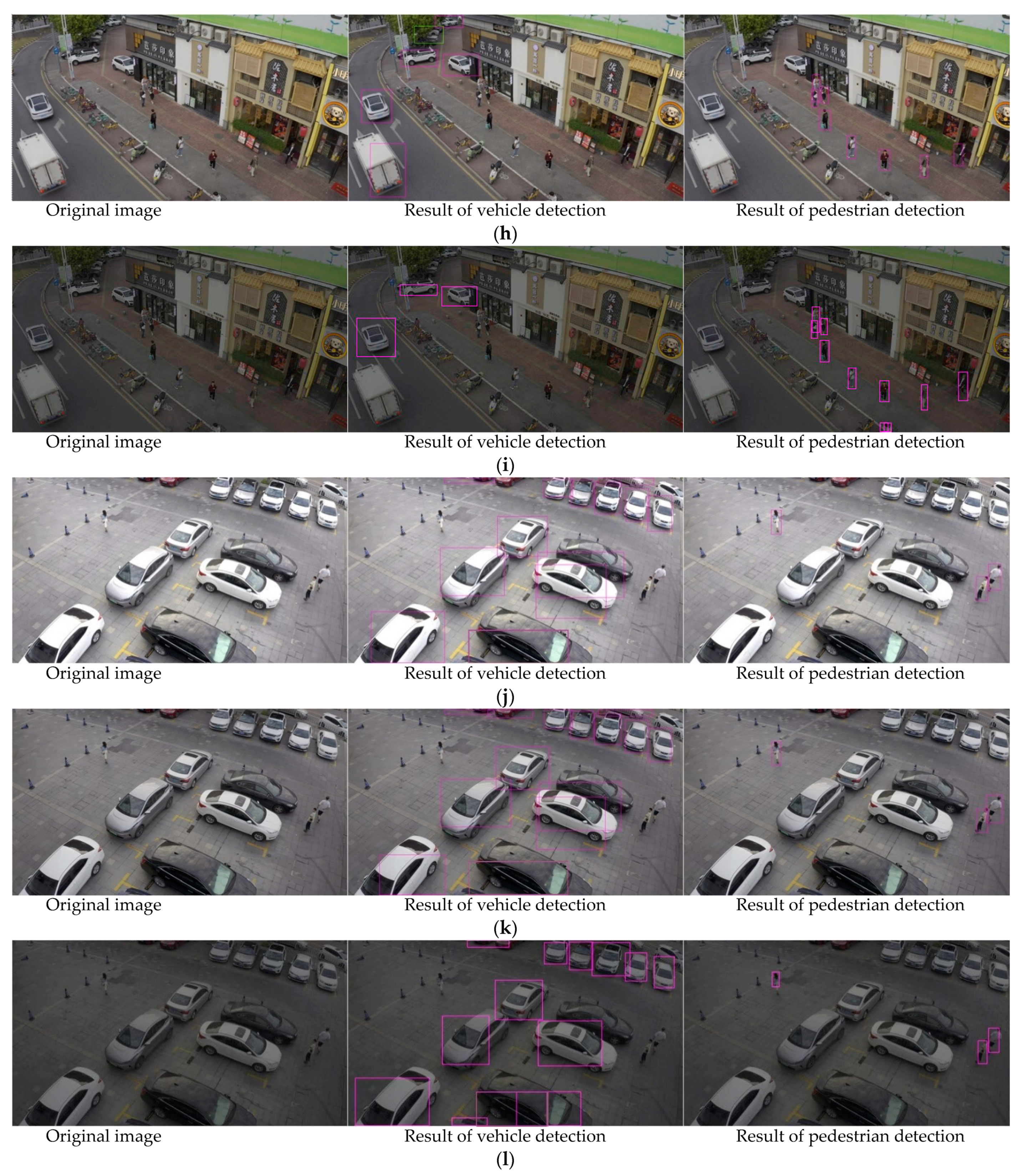
2.3. The Ground Pedestrian and Vehicle Detection

After environment perception, three kinds of luminance can be obtained: excellent, ordinary, and severe. To obtain a robust classification, we distinguish the network designs of pedestrians and vehicles with the consideration of different imaging luminance.

Table 2. Definitions of imaging luminance degrees.

	Imaging Luminance Degree
	Excellent	Ordinary	Severe
The environment light intensity	~≥1500 lx	~≥300 lx and ~<1500 lx	~≥50 lx and ~<300 lx
The information entropy	HL > 4.8, 2.8 > Ha > 1.5, and 2.5 > Hb ≥ 1.0	5.0 > HL ≥ 3.7, 2.9 > Ha ≥ 1.7, and 2.2 > Hb ≥ 1.3	4.8 > HL ≥ 2.8, 3.6 > Ha ≥ 1.0, 2.0 > Hb ≥ 1.2

presents the definition of imaging luminance degree. In Table 2, the imaging luminance degrees are defined by both the environment light intensities and information entropy values.

Regarding ground pedestrian detection, the network input is set by 544 × 544 because of the small pedestrian sizes. When imaging luminance is excellent, 1 × 1 and 3 × 3 convolutional layers are added after the third and the fourth convolutional layers of Yolov3-tiny. An upsample2 layer is added in the ninth convolutional layer. Moreover, the outputs of feature pyramid layers become 136 × 136 × 18, 68 × 68 × 18, and 34 × 34 × 18, respectively. When imaging luminance is ordinary, six convolutional layers (i.e., 1 × 1, 3 × 3, 1 × 1, 3 × 3, 1 × 1, and 3 × 3) are added after the third layer of Yolov3-tiny. The 5 × 5, 9 × 9, and 13 × 13 SPP layers are considered after the fourth convolutional layer. Moreover, a 136 × 136 prediction structure was also utilized. When imaging luminance is severe, a dense block is used to replace the second convolutional layer of Yolov3-tiny; 1 × 1, 3 × 3 and 1 × 1 convolutional layers were added after the third convolutional layer. SPP is considered for each prediction structure, and a 136 × 136 prediction structure was also utilized.

As for ground vehicle detection, the network input is set by 512 × 512 for the comparably large sizes of vehicles. When imaging luminance is excellent, more details will be obtained if the network’s resolution can be improved; thus, we delete two prediction structures of Yolov3-tiny in front, add a bi-directional feature pyramid network (BiFPN), and set 32 × 32 and 64 × 64 prediction structures in the end. The 1 × 1 and 3 × 3 convolutional layers are also considered for improving the detail detection ability of the network. When imaging luminance is ordinary, the details of vehicles become obscure; thus, 1 × 1 and 3 × 3 convolutional layers were added after the third and the fourth layers of the Yolov3-tiny network. An SPP structure that uses 5 × 5, 9 × 9, and 13 × 13 maximum pooling layers is also added after the seventh convolutional layer. When imaging light is severe, the network depth should be improved to obtain a stable detection effect. The feature collection structure of DenseNet [40] is used to replace the feature extraction layer of Yolov3-tiny, and an SPP layer is also employed in our model.

Figure 3 shows the structures of our proposed networks. The blocks marked by blue or red color are the modules proposed by us. Clearly, significant changes are made in these models. A DCBlock and an OPBlock were developed to replace the initial single convolutional layer of Yolov3-tiny; then, the features coming from previous layer can be reused and recombined properly. The design concepts are derived from the residual learning technique [41]. It is difficult to extract the features of different scales by using a single convolution layer; thus, an SPP module is used for multi-scale feature extraction and integration. This module is mainly composed of four parallel paths, i.e., one shortcut connection and three maximum pool layers. The core sizes are 5 × 5, 9 × 9, and 13 × 13. Then, a connection layer is set up to combine the characteristics of four paths as the final output. With the application of the SPP module, the features of different scales are extracted and integrated in one step, which can enhance the detection performance of the network. Finally, our network also adds dense block modules to Yolov3-tiny in order to fully reuse multi-layer features.

3. Experiments and Results

A series of tests and evaluation experiments was performed to assess the effectiveness of the proposed method. All simulation programs were written by Python (Pycharm2020) in our PC (4.0 GB RAM, 1.70 GHz Intel (R) Core (TM) i3-4005 U CPU).

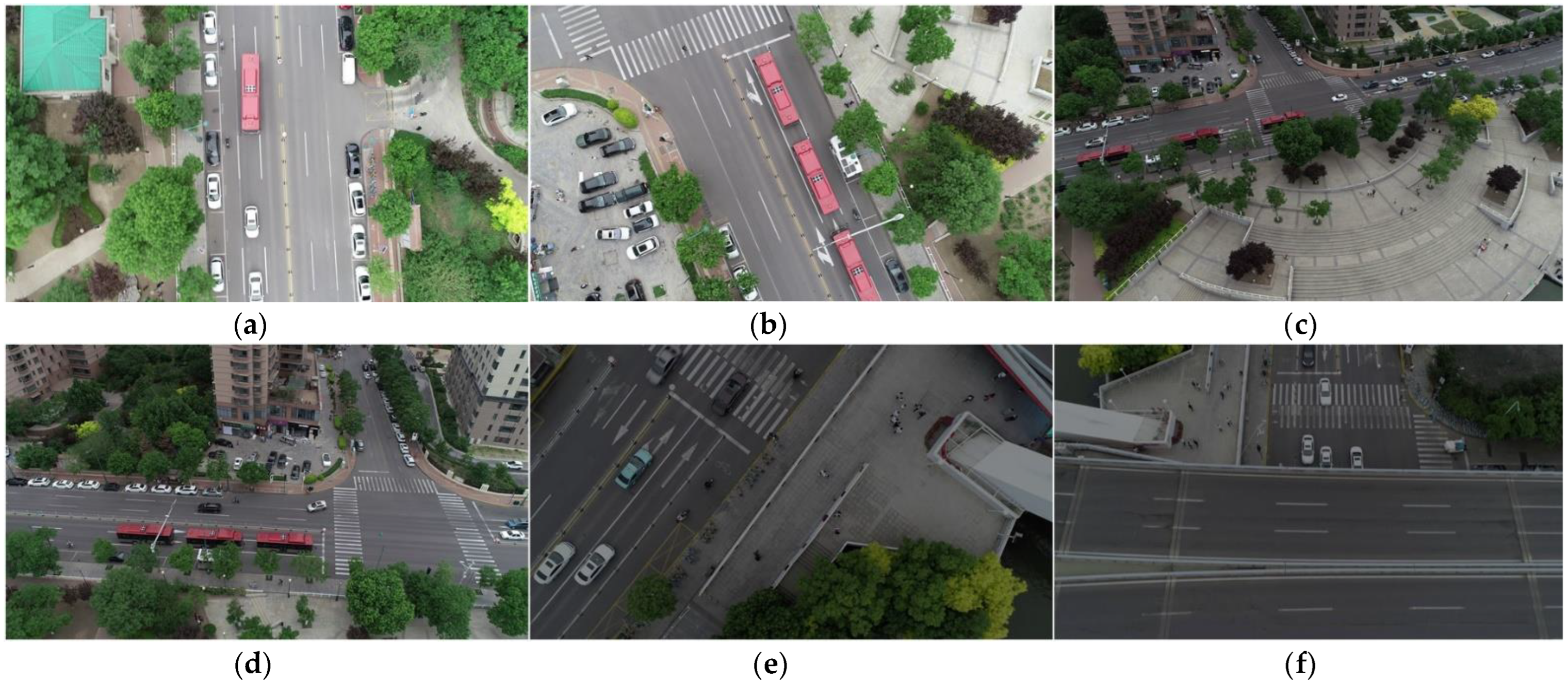
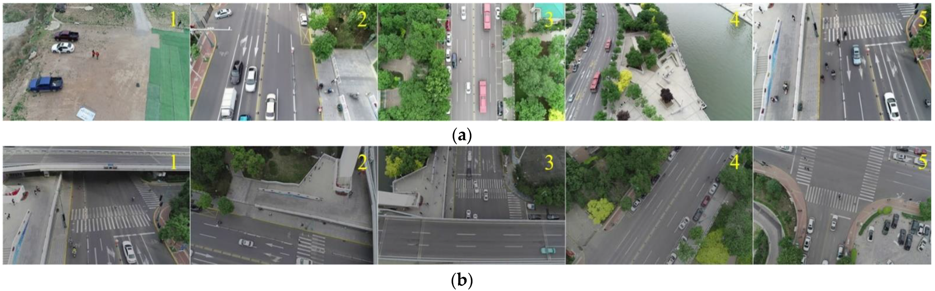
3.1. Experiment Data Collection and Orgnization

A commercial UAV was used to collect ground data under different environment luminance. The images captured during the daytime in summer and in Beijing and Shunde, China, were accumulated. Figure 4 presents an example of the image data. In Figure 4, (a) and (b) are the image samples that have excellent imaging luminance; (c) and (d) are the samples that have ordinary imaging luminance; (e) and (f) are the samples that have severe imaging luminance. From Figure 4, the degradation of imaging luminance comes from the change in environment luminance or change in photographic altitude from light sources (e.g., the sun light source or ground light reflection source, etc.). Clearly, in this study, poor environment luminance will create weak imaging luminance, while weak imaging luminance can also come from excellent environment luminance. In order to expand the size of training dataset, image degradation processing was also designed and performed. Equation (5) shows our computational method:

$$I_2(i,j)=n_1\times I_1(i,j)+n_2$$

(5)

where I₁(i, j) is the original image pixel in (i, j), which is always captured from excellent imaging luminance environments; I₂(i, j) is the degraded image pixel in (i, j); symbols n₁ and n₂ are the parameters. In this study, regarding ordinary luminance, n₁ = 1.1 and n₂ = 7; as for severe luminance, n₁ = 1.24 and n₂ = 8. Moreover, with respect to excellent luminance, n₁ = 1.0 and n₂ = 0.0.

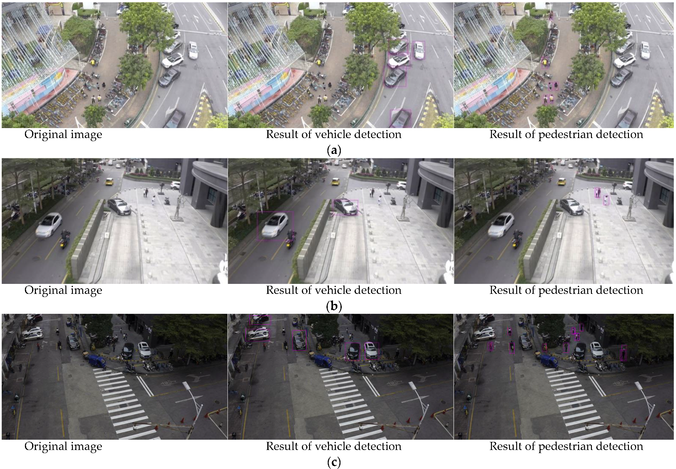
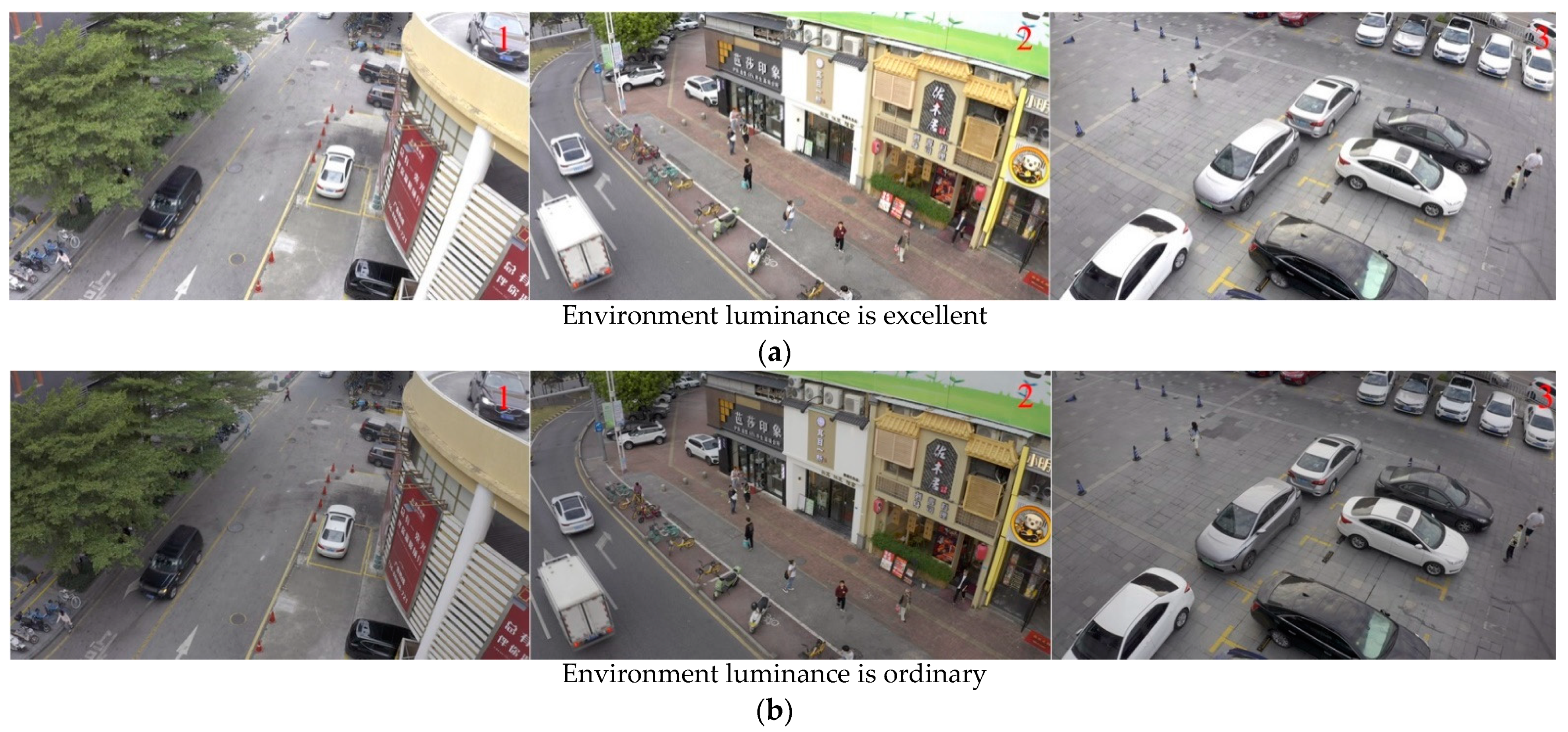
3.2. Evaluation of Environment Perception Method

A series of computations was performed to implement imaging environment perception. First, typical image data were selected and tagged from the original UAV dataset. Figure 5 presents the image samples. In Figure 5, (a) is the image samples captured with excellent imaging luminance effects; (b) and (c) show data collected from ordinary and severe imaging effects, respectively. Second, an evaluation experiment involving the SVM classifier was performed.

Table 3. Accuracy comparison of different SVM construction methods.

Kernel Function	Polynomial Function	Linear Function	Sigmoid Function	Radial Basis Function
Classification Accuracy	89.88%	89.91%	86.83%	94.18%

presents the results. In this experiment, the selected UAV dataset above was used to train SVM; the training data amount of SVM was 4116, and the test data amount was 4116. In Table 3, the classification accuracies using different kernel functions [46] were investigated; the experiment’s results show that the radial basis function-based method can obtain the best processing effects. Third, SVM-based environment perception computations and subjective imaging luminance evaluations were performed.

Table 4. Results of information entropy indices, SVM output, and subjective imaging luminance evaluation.

Image Name	HL	Ha	Hb	SVM Output	Subjective Imaging Luminance Evaluation Result
Figure 5(a1)	5.0249	2.3291	1.6198	Excellent	Excellent
Figure 5(a2)	4.8127	1.9634	1.9739	Excellent	Excellent
Figure 5(a3)	4.9405	2.7008	2.4635	Excellent	Excellent
Figure 5(a4)	4.9211	2.4632	1.9028	Excellent	Excellent
Figure 5(a5)	4.8957	2.0603	1.7359	Excellent	Excellent
Figure 5(b1)	3.8071	1.9116	1.5406	Ordinary	Ordinary
Figure 5(b2)	4.1549	2.3701	1.6831	Ordinary	Ordinary
Figure 5(b3)	3.7945	1.7859	1.380	Ordinary	Severe
Figure 5(b4)	4.2191	3.3829	2.1078	Ordinary	Ordinary
Figure 5(b5)	4.4361	2.3164	1.6128	Ordinary	Ordinary
Figure 5(c1)	4.6073	3.6122	1.6468	Severe	Severe
Figure 5(c2)	2.8561	1.6391	1.3944	Severe	Severe
Figure 5(c3)	3.0664	1.1879	1.4347	Severe	Severe
Figure 5(c4)	4.0096	1.7767	2.0469	Severe	Severe
Figure 5(c5)	3.6726	1.4922	1.5965	Severe	Severe

illustrates the results of information entropy (H_L, H_a, and H_b), SVM output, and the subjective evaluation of imaging luminance degree. The subjective evaluation results came from the subjects’ votes of imaging luminance degree, and the average vote values were used in this experiment. Similarly, the vote degrees also have three levels: excellent, ordinary, and severe. From Table 4, subjective and objective assessments can obtain a similar result; thus, we think our method can obtain a comparable stable processing effect.

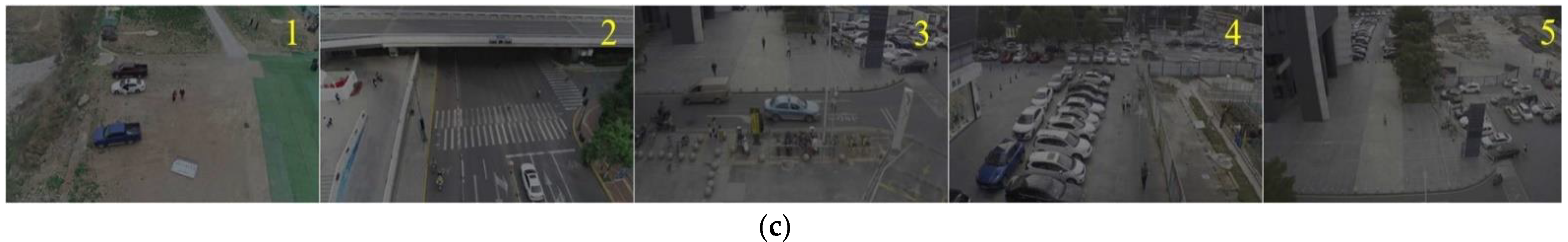
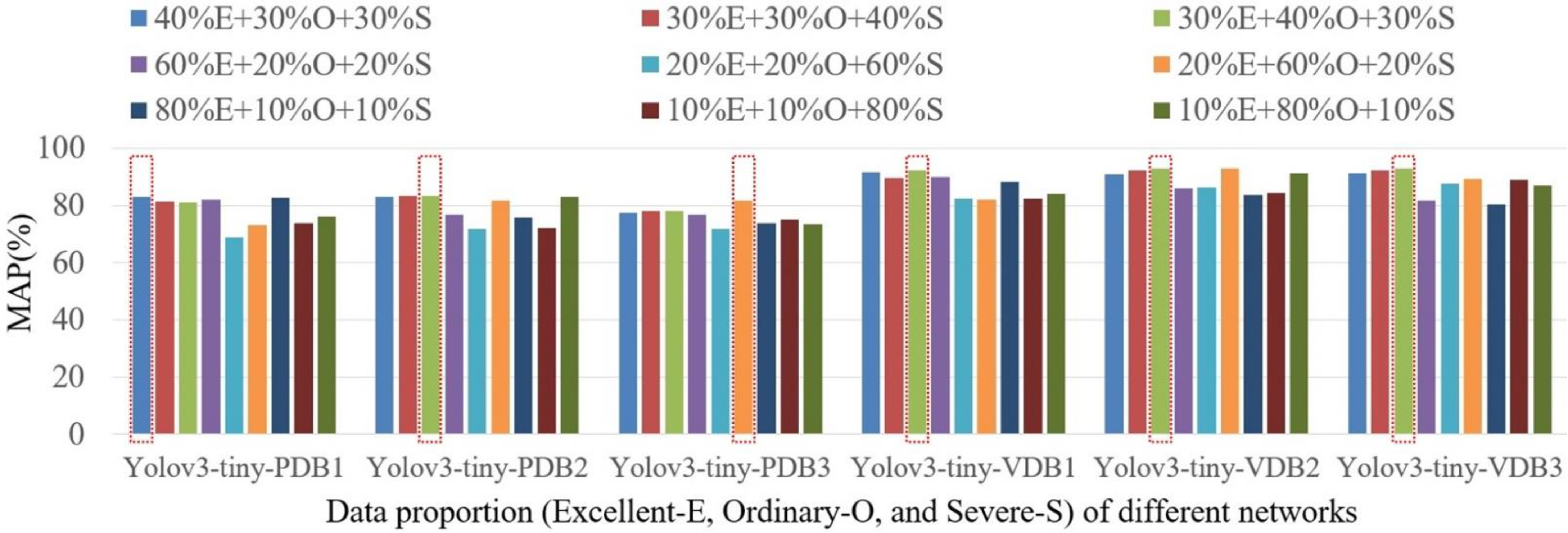
3.3. Evaluation of Ground Pedestrian and Vehicle Detection Methods

The experimental comparisons were made to evaluate the effectiveness of the proposed pedestrian and vehicle detection methods. Twelve deep learning-based networks were compared: Yolov3-tiny-PDB1, Yolov3-tiny-PDB2, Yolov3-tiny-PDB3, Yolov3-tiny-VDB1, Yolov3-tiny-VDB2, Yolov3-tiny-VDB3, Yolov3-tiny, Yolov4+Mobilenetv3 [47], Efficientnet-B0 [48], RetinaNet [22], CenterNet [24], and SSD [49]. After a series of tests, all evaluated networks could be used in the real time computation of UAV applications. Mobilenetv3 is a network that considers both depthwise separable convolution and attention mechanisms. Automatic machine learning techniques, including MnasNet and NetAdapt, are utilized. Efficientnet-B0 is an architecture that uses MnasNet with the consideration of excitation optimization in MBConv layers to build its network. The compound scaling method is utilized in this model. RetinaNet is designed to solve the focal loss problem of traditional networks. The unbalanced category issue can be handled well by this network. CenterNet is a kind of anchor-free network; moreover, apparent improvements have been made in its network structure, heatmap generation, and data enhancement. The SSD method employs a multi-scale default box to generate a feature map. It provides good performance in real-time computation in many applications. Because Yolo-family networks have similar processing mechanisms and computational effects, they are not compared much in this experiment.

Table 5. Detection accuracy comparisons using different deep learning networks and test datasets.

MAP(%)/ Recall(%)	Network Type
	Yolov3- Tiny-PDB1	Yolov3- Tiny-PDB2	Yolov3- Tiny-PDB3	Yolov3- Tiny-VDB1	Yolov3- Tiny-VDB2	Yolov3- Tiny-VDB3	Yolov3- Tiny	Yolov4+ Mobilenetv3	Efficientnet -B0	Retina Net	Center Net	SSD
Mixture dataset1 a	81.10/ 68.95	82.13/ 71.39	77.64/ 55.73	-	-	-	77.94/ 79.27	76.56/ 74.97	68.52/ 57.71	42.03/ 20.04	75.57/ 49.32	47.36/ 11.49
Mixture dataset2	-	-	-	87.76/ 74.33	91.89/ 84.73	90.33/ 76.58	91.54/ 88.24	89.88/ 77.90	86.64/ 72.85	86.14/ 71.07	86.51/ 46.57	88.98/ 60.37
Typical dataset1	85.36/ 74.69	82.50/ 73.86	78.17/ 73.31	-	-	-	73.21/ 71.26	78.67/ 76.06	76.01/ 51.84	39.68/ 18.50	81.80/ 36.28	49.38/ 8.95
Typical dataset2	80.09/ 72.58	84.75/ 82.21	77.04/ 54.97	-	-	-	70.43/ 70.08	75.52/ 76.90	66.02/ 43.15	38.96/ 18.14	82.65/ 44.74	46.07/ 13.24
Typical dataset3	77.76/ 66.39	76.59/ 71.18	79.15/ 67.32	-	-	-	68.31/ 67.49	77.09/ 71.83	64.78/ 40.57	36.99/ 15.84	78.12/ 56.91	33.07/ 5.08
Typical dataset4	-	-	-	94.29/ 76.83	90.21/ 90.03	90.77/ 79.62	92.47/ 91.41	93.34/ 91.98	83.39/ 75.40	84.07/ 68.37	91.96/ 79.24	91.16/ 61.51
Typical dataset5	-	-	-	90.46/ 78.14	94.26/ 91.25	92.93/ 86.96	92.14/ 92.81	92.61/ 90.05	82.61/ 72.68	83.99/ 69.23	89.67/ 75.86	90.53/ 62.07
Typical dataset6	-	-	-	87.76/ 74.33	92.57/ 92.07	94.48/ 90.79	91.66/ 92.17	92.33/ 89.46	80.77/ 67.71	82.87/ 67.24	89.59/ 66.78	90.33/ 61.41

^a Mixture dataset1 and Mixture dataset2 were designed for pedestrian and vehicle detections respectively, where imaging luminance with all kind of situations (i.e., the proportions of different luminance image datasets are equal) was used. Typical dataset1 and dataset4 were designed for pedestrian and vehicle detections when imaging luminance is excellent. Typical dataset 2 and dataset 5 were designed for pedestrian and vehicle detections when imaging luminance is normal. Typical dataset3 and dataset6 were designed for pedestrian and vehicle detections when imaging luminance is severe.

provides the corresponding results using different deep learning networks and test datasets. In Table 5, a series of datasets was used for network evaluation: Mixture datasets do not distinguish imaging luminance and use all accumulated image data to train networks (i.e., the proportions of three types of image dataset are equal); the typical datasets only consider image data with the same imaging luminance to build their training and test datasets. In this experiment, the sizes of the training datasets (including the Mixture dataset1, Typical dataset1, Typical dataset2, and Typical dataset3) of pedestrian detection are all 2354; the corresponding test data sizes are all 262; the sizes of training datasets (including the Mixture dataset2, Typical dataset4, Typical dataset5, and Typical dataset6) of vehicle detection are all 2219, the corresponding test data sizes are all 555. From Table 5, regarding mixture datasets, our networks (including both Yolov3-tiny-PDB2 and Yolov3-tiny-VDB2) for ordinary luminance application can obtain the best results among all networks. As for the image data captured in typical luminance degrees, our networks also can obtain the best processing effects in their individual test experiments.

Table 6. Average processing time comparison using different deep learning networks.

	Yolov3- Tiny-PDB1	Yolov3- Tiny-PDB2	Yolov3- Tiny-PDB3	Yolov3- Tiny-VDB1	Yolov3- Tiny-VDB2	Yolov3- Tiny-VDB3	Yolov3- tiny	Yolov4+ Mobilenetv3	Efficientnet -B0	Retina Net	Center Net	SSD
Processing time (ms/frame)	4.154	5.380	6.798	5.251	5.416	7.448	3.874	14.259	100.274	65.239	22.359	52.632

shows the computational speeds of all networks in Table 5. From Table 6, our networks can accomplish pedestrian and vehicle detections within 8.0 ms per frame. Figure 6 presents examples of ground pedestrian and vehicle detection results of our proposed method, and images with different scenes and environment luminance are used. In Figure 6, a purple rectangle is used to mark the detected vehicle and pedestrian. Figure 7 shows the processing examples of images with the same scene but different environment luminance. In Figure 7, although imaging luminance is different, the detection results are the same. From Figure 6 and Figure 7, our method can detect most pedestrians and vehicles in complex scenes with different environment luminance degrees.

An ablation analysis experiment was performed to test the validity of proposed networks. In general, regarding the ablation analysis experiment, the modules in the original model will be removed or replaced one-by-one in order to build a new network structure; then, performance evaluations will be conducted for the new networks. As for the Yolov3-tiny network, to maintain its basic network structure, only the elimination operation was considered in this experiment.

Table 7. Ablation analysis results using different networks and datasets.

Network Description	Dataset Description	MAP(%)/Recall(%)
Yolov3-tiny_VDB1	Data of vehicle detection experiment; the data proportions of excellent, ordinary, and severe luminance degrees are 100%, 0%, and 0%.	94.29/76.83
Yolov3-tiny_VDB1 without module 1.		87.86/72.36
Yolov3-tiny-VDB1 without modules 1 and 2.		86.68/69.83
Yolov3-tiny-VDB1 without modules 1, 2, and 3.		83.86/64.85
Yolov3-tiny-VDB1	Data of vehicle detection experiment; the data proportions of excellent, ordinary, and severe luminance degrees are equal.	87.76/74.33
Yolov3-tiny_VDB1 without module 1.		87.54/71.53
Yolov3-tiny-VDB1 without modules 1 and 2.		86.03/66.16
Yolov3-tiny-VDB1 without modules 1, 2, and 3.		84.19/70.55
Yolov3-tiny-PDB1	Data of pedestrian detection experiment; the data proportions of excellent, ordinary, and severe luminance degrees are 100%, 0%, and 0%.	85.36/74.69
Yolov3-tiny-PDB1 without module 1.		71.79/66.19
Yolov3-tiny-PDB1 without modules 1 and 2.		69.28/59.32
Yolov3-tiny-PDB1	Data of pedestrian detection experiment; the data proportions of excellent, ordinary, and severe luminance degrees are equal.	81.10/68.95
Yolov3-tiny-PDB1 without module 1.		69.48/59.67
Yolov3-tiny-PDB1 without modules 1 and 2.		66.13/54.20
Yolov3-tiny-VDB2	Data of vehicle detection experiment; the data proportions of excellent, ordinary, and severe luminance degrees are 0%, 100%, and 0%.	94.26/91.25
Yolov3-tiny-VDB2 without module 1.		91.91/83.72
Yolov3-tiny-VDB2 without modules 1 and 2.		91.27/83.02
Yolov3-tiny-VDB2	Data of vehicle detection experiment; the data proportions of excellent, ordinary, and severe luminance degrees are equal.	91.89/84.73
Yolov3-tiny-VDB2 without module 1.		90.69/86.96
Yolov3-tiny-VDB2 without modules 1 and 2.		87.20/72.58
Yolov3-tiny-PDB2	Data of pedestrian detection experiment; the data proportions of excellent, ordinary, and severe luminance degrees are 0%, 100%, and 0%.	84.75/82.21
Yolov3-tiny-PDB2 without module 1.		67.94/56.55
Yolov3-tiny-PDB2 without modules 1 and 2.		70.49/59.67
Yolov3-tiny-PDB2	Data of pedestrian detection experiment; the data proportions of excellent, ordinary, and severe luminance degrees are equal.	82.13/71.39
Yolov3-tiny-PDB2 without module 1.		65.31/55.89
Yolov3-tiny-PDB2 without modules 1 and 2.		66.81/54.01
Yolov3-tiny-VDB3	Data of vehicle detection experiment; the data proportions of excellent, ordinary, and severe luminance degrees are 0%, 0%, and 100%.	94.48/90.79
Yolov3-tiny-VDB3 without module 1.		89.78/75.57
Yolov3-tiny-VDB3	Data of vehicle detection experiment; the data proportions of excellent, ordinary, and severe luminance degrees are equal.	90.33/76.58
Yolov3-tiny-VDB3 without module 1.		82.24/61.49
Yolov3-tiny-PDB3	Data of pedestrian detection experiment; the data proportions of excellent, ordinary, and severe luminance degrees are 0%, 0%, and 100%.	79.15/67.32
Yolov3-tiny-PDB3 without module 1.		48.01/34.89
Yolov3-tiny-PDB3 without modules 1 and 2.		43.32/22.95
Yolov3-tiny-PDB3 without modules 1, 2, and 3.		37.91/26.69
Yolov3-tiny-PDB3	Data of pedestrian detection experiment; the data proportions of excellent, ordinary, and severe luminance degrees are equal.	77.64/55.73
Yolov3-tiny-PDB3 without module 1.		37.70/20.31
Yolov3-tiny-PDB3 without modules 1 and 2.		32.75/11.97
Yolov3-tiny-PDB3 without modules 1, 2, and 3.		30.01/12.61

presents the corresponding results. As stated above, Figure 3 illustrates the structures of our proposed improved Yolov3-tiny networks; the dashed boxes and their red numbers mark the replaceable modules of the ablation experiment. In Table 7, both the typical datasets and the mixture datasets, i.e., the same datasets in Table 5, were used for MAP and recall evaluations. When implementing the ablation experiment, the modules in dashed boxes were first removed (i.e., implementing the elimination operation) one-by-one; then, typical or mixture datasets were used to test the remaning networks. From Table 7, our proposed networks can obtain the best detection results, and the best results of different networks are also marked in bold.

An evaluation experiment using different proportions of various imaging quality data was carried out. Figure 8 presents the corresponding results. In Figure 8, different data proportions were considered: 40%/30%/30%, 60%/20%/20%, and 80%/10%/10%. The selection of these data proportions comes from our application experiences: Many of our experiment results have shown that the approximately equal proportion of three types of training data (i.e., the data collected from the excellent, ordinary, and severe luminance conditions) will result in a high network detection effect; thus, in this experiment, we only selected different data combination modes with large proportion differences to test and verify this hypothesis above. Furthermore, this experience can assess the MAP index when the proportions of different data types are approximate equal or when they have large quantity deviations. In Figure 8, for example, “30%E + 30%O + 40%S” means that we use 30% image data with excellent luminance effect, 30% data with ordinary luminance effect, and 40% data with severe luminance effect to build the experimental dataset. Our trained and improved Yolov3-tiny networks were utilized in this experiment. The test data amounts of pedestrian and vehicle detections were 250 and 550, respectively. The largest MAP values of each network are marked by red dash rectangles. From Figure 8, regarding pedestrian detection networks, when data proportions are 40%E + 30%O + 30%S, 30%E + 40%O + 30%S, and 20%E + 60%O + 20%S, the best MAP can be obtained. This result may indicate that a high pedestrian detection rate can be obtained when the proportions of different data types are approximate equal or ordinary luminance dataset can play an important role among these datasets. As for vehicle detection networks, the corresponding networks can obtain the best processing effect when the data proportion is 30%E + 40%O + 30%S. This result also displays the best performance of approximate equal data combination modes. The best result can be found when the proportion of ordinary luminance image is the largest.

3.4. Discussions

UAV ground target detection has wide application prospects [50] in intelligent transportation, crowd management, and crime prevention, etc. Regarding smart city construction, the main difficulties in the application of this type of technique comes from the negative influence of environment luminance and the atmosphere [51]; the response ability of optic devices will be seriously degraded by these factors, and then it will affect the following image processing algorithm in many cases. Multispectral camera or multi-camera systems can be used to solve this problem to some extent; however, their set up costs are very high. Recently, low-cost visible light cameras combined with deep learning network-based detection algorithms have been used to solve this particular task; the main drawbacks of this method is collecting the large amount of training data and slow network training speeds, which limit their applications. In this study, a two-thread computation method was developed: One thread is used to monitor and evaluate imaging luminance changes; the other thread is considered for robust ground target detection according to the assessment result of environment perceptions. With the guidance of imaging quality analysis, a variety of lightweight deep learning networks can be employed for real-time ground target detection.

As we all know, the main difficulty in the application of visible light camera under outdoor conditions comes from the change of complex environmental light; this problem is apparent, particularly in the application of UAV systems. Suspended particles in the air can scatter and absorb sunlight, and the response ability of ordinary cameras under high environment brightness (pixel linear response ability, noise suppression ability, etc.) is generally better than that obtained under low environment brightness degrees, which will always lead to the phenomena of low imaging contrast and blurred edge when we observe ground targets from longer distances. Clearly, during the day, the changes in skylight follow significant laws. According to the analysis of different weather conditions, we can distinguish the impact of different imaging environments on the final output of the camera effectively. In this paper, our system adopts a high-definition motion camera, and the UAV only performs slow-speed flight tasks; other problems, such as motion blur or defocus blur, will hardly appear in the process of system applications. Therefore, the final environmental perception calculation in this paper mainly considers the estimation of environmental brightness. Table 2 and Figure 5 present the definitions and examples of images captured under different environment luminance degrees. In the future, more image data will be accumulated in our system to improve the accuracy of imaging luminance computation.

Many image quality evaluation metrics could be used for environment perception; however, considering both the processing speed and analysis effect, only entropy-based imaging luminance evaluation metrics were used in this study. In general, the edge detail, region contrast, or image noise [52] will affect image quality of the ground targets; however, their complex computations will restrict system applications in engineering. MSCN values can reduce the mean shift and restrain the local variance of contrast information; then, the relevance among pixels can be weakened. Since entropy is always used for texture analysis and the application of high-definition cameras will not meet strong image noise, as a result, the sequential computations of MSCN values and entropy can reflect imaging luminance rather than contrast or other details. The processing speeds of proposed method are also computed when multi-factor evaluation (the edge blur, region contrast, and imaging noise) [5] and our single factor evaluation assessment (entropy-based imaging luminance) are used for perception. The experiment result shows that the multi-factor method [5,53] will use ~0.0643 s while our method will only spend ~ 0.0347 s to accomplish imaging environment perception computations for each image. This result can indicate the advantage of our method to some extent.

The lightweight deep learning network [54] was considered in this study for convenient UAV applications. The main merits of this type of network consist in its small requirement of training data and short consumption time periods for network training. It is well known that the transfer learning network [55] can solve training issues related to a small amount of experimental data too. Transfer learning uses a priori information and pre-training networks to reduce data collection costs and training resource consumption. Transfer learning holds the assumption that the new untrained network has the same or similar data distribution relative to the pre-training network. Unfortunately, this assumption is not true in many practical applications because the distribution of new datasets is always unknown. Clearly, the construction of a pre-training network also is a complex task in practice. In this study, our evaluation experiments show the following: Although some transfer learning methods (such as pre-training in addition to training full connection layers or pre-training in addition to training grouping convolutions, full connection layer, and batch normalization layer) can obtain better detection accuracies than the lightweight network, they do not fit the fast application requirements of a city’s administration department. As a result, the proposed improved Yolov3-tiny networks are utilized in this study.

Another problem for ground pedestrian and vehicle recognition is the image noise reduction issue. For UAVs, environmental factors, such as complex air medium, ground electromagnetic wave interference, and changeable environment light, will lead to all types of noise. Common noise will cause the loss of edge details and a lack of feature and texture details in aerial images. These problems will have a particularly significant impact on small aerial target detections. In order to solve the problems above to a certain extent, on the one hand, the camera system with higher resolution, high dynamic range, and low system noise should be selected as much as possible from the perspective of hardware system design; on the other hand, noise analyses and reduction technologies [56,57] such as the edge-preservation filtering need to be investigated. The design of relevant fast algorithms also should be considered in order to meet the needs of UAV aerial photography. Regarding the noise reduction problem, this paper mainly improves the input aspect ratio of our improved Yolov3-tiny network and appropriately designs the noise reduction module to achieve highly robust feature extraction and noise suppression. DCBlock and OPBlock inherited the structure of residual networks, which can solve the problem of detailed feature loss and suppress background noise well. Through the dense connection between layers, Denseblock can consider local information and play an important role in suppressing background noise.

The proposed method has at least three advantages. First, its computational stability is comparably high. Because of the application of imaging luminance analysis (i.e., the environment perception computation [58]), deep learning networks can be selected intelligently according to environment luminance changes; moreover, the environment’s adaptability toward target detection algorithms can be improved dramatically. Second, the usability of the proposed method is good. In this study, many lightweight deep learning networks were used, and only a small amount of training data were needed. This merit can reduce the workload of training data collection and decrease the consumption of time during network training, both of which are fit for emergency applications of UAVs. Third, the expandability of this system is also excellent. Clearly, different environment perception metrics and some other lightweight deep learning networks can also be considered to replace current entropy-based metrics and improved Yolov3-tiny networks [59]. Our proposed method also has some shortcomings. For example, in order to reduce the computational complexity of environment perception, only the basic information entropy function was used; actually, the entropy estimation method in other data space [60] can be considered in our system in the future. In the next step, a special integrated circuit system will be developed for our proposed method to realize an onboard computation.

4. Conclusions

A robust ground pedestrian and vehicle detection method for UAV applications was proposed. Both environment perception computations and deep learning network detections were considered in this method. First, imaging luminance descriptors were estimated: MSCN values were computed for each color component after the initial image data were transformed from RGB to Lab color space; then, information entropies were calculated by using the MSCN values listed above. Second, SVM was used to implement a fast imaging luminance classification. Its inputs include three information entropy indices, and its output is the imaging luminance degree. Third, six improved lightweight Yolov3-tiny networks were designed for ground pedestrian and vehicle detections under three types of imaging luminance degrees. Some highly efficient network structures, such as DCBlock, OPBlock, and Denseblock, were proposed or used in our models. Extensive experiment results have illustrated that the MAPs of pedestrian and vehicle detections are better than ~80% and ~94%, respectively. In the future, more environment perception metrics will be designed and other lightweight deep learning networks will be considered for real-time UAV applications.

References

1. Zhang, F.; Xu, Z.; Chen, W.; Zhang, Z.; Zhong, H.; Luan, J.; Li, C. An image compression method for video surveillance system in underground mines based on residual networks and discrete wavelet transform. Electronics 2019, 8, 1559. [Google Scholar] [CrossRef] [Green Version]
2. Nawaratne, R.; Kahawala, S.; Nguyen, S.; De Silva, D. A generative latent space approach for real-time surveillance in smart cities. IEEE Trans. Ind. Inform. 2021, 17, 4872–4881. [Google Scholar] [CrossRef]
3. Li, X.; Yu, Q.; Alzahrani, B.; Barnawi, A.; Alhindi, A.; Alghazzawi, D.; Miao, Y. Data fusion for intelligent crowd monitoring and management systems: A survey. IEEE Access 2021, 9, 47069–47083. [Google Scholar] [CrossRef]
4. Kim, H.; Kim, S.; Yu, K. Automatic extraction of indoor spatial information from floor plan image: A patch-based deep learning methodology application on large-scale complex buildings. ISPRS Int. J. Geo Inf. 2021, 10, 828. [Google Scholar] [CrossRef]
5. Liu, H.; Yan, B.; Wang, W.; Li, X.; Guo, Z. Manhole cover detection from natural scene based imaging environment perception. KSII Trans. Internet Inf. Syst. 2019, 13, 5059–5111. [Google Scholar]
6. Honkavaara, E.; Eskelinen, M.A.; Polonen, I.; Saari, H.; Ojanen, H.; Mannila, R.; Holmlund, C.; Hakala, T.; Litkey, P.; Rosnell, T.; et al. Moisture of a peat production area using hyperspectral frame cameras in visible to short-wave infrared spectral ranges onboard a small unmanned airborne vehicle (UAV). IEEE Trans. Geosci. Remote Sens. 2016, 54, 5440–5454. [Google Scholar] [CrossRef] [Green Version]
7. Gao, T.; Li, K.; Chen, T.; Liu, M.; Mei, S.; Xing, K.; Li, Y. A novel UAV sensing image defogging method. IEEE J STARS 2020, 13, 2610–2625. [Google Scholar] [CrossRef]
8. Khelifi, L.; Mignotte, M. Deep learning for change detection in remote sensing images: Comprehensive review and meta-analysis. IEEE Access 2020, 8, 126385–126400. [Google Scholar] [CrossRef]
9. Ezeme, O.M.; Mahmoud, Q.H.; Azim, A.A. Design and development of AD-CGAN: Conditional generative adversarial networks for anomaly detection. IEEE Access 2020, 8, 177667–177681. [Google Scholar] [CrossRef]
10. Azar, A.T.; Koubaa, A.; Mohamed, N.A.; Ibrahim, H.A.; Ibrahim, Z.F.; Kazim, M.; Ammar, A.; Benjdira, B.; Khamis, A.M.; Hameed, I.A.; et al. Drone deep reinforcement learning: A review. Electronics 2021, 10, 999. [Google Scholar] [CrossRef]
11. Liu, C.; Wu, Y.; Liu, J.; Sun, Z. Improved YOLOv3 network for insulator detection in aerial images with diverse background interference. Electronics 2021, 10, 771. [Google Scholar] [CrossRef]
12. Ammar, A.; Koubaa, A.; Ahmed, M.; Saad, A.; Benjdira, B. Vehicle detection from aerial images using deep learning: A comparative study. Electronics 2021, 10, 820. [Google Scholar] [CrossRef]
13. Vasic, M.K.; Papic, V. Multimodel deep learning for person detection in aerial images. Electronics 2020, 9, 1459. [Google Scholar] [CrossRef]
14. Shen, Z.; Liu, Z.; Li, J.; Jiang, Y.-G.; Chen, Y.; Xue, X. Object detection from scratch with deep supervision. IEEE Trans. Pattern Anal. 2020, 42, 398–412. [Google Scholar] [CrossRef] [PubMed] [Green Version]
15. Haroun, F.M.E.; Deros, S.N.M.; Din, N.M. Detection and monitoring of power line corridor from satellite imagery using RetinaNet and K-mean clustering. IEEE Access 2021, 9, 116720–116730. [Google Scholar] [CrossRef]
16. Rao, Y.; Yu, G.; Xue, J.; Pu, J.; Gou, J.; Wang, Q.; Wang, Q. Light-net: Lightweight object detector. IEEE Access 2020, 8, 201700–201712. [Google Scholar] [CrossRef]
17. Duan, K.; Bai, S.; Xie, L.; Qi, H.; Huang, Q.; Tian, Q. CenterNet: Keypoint triplets for object detection. In Proceedings of the IEEE/CVF International Conference on Computer Vision (ICCV’19), Seoul, Korea, 27 October–2 November 2019; pp. 6568–6577. [Google Scholar]
18. Mekhalfi, M.L.; Nicolo, C.; Bazi, Y.; Rahhal, M.M.A.; Alsharif, N.A.; Maghayreh, E.A. Contrasting YOLOv5, transformer, and EfficientDet detectors for crop circle detection in desert. IEEE Geosci. Remote Sens. 2022, 19, 205. [Google Scholar] [CrossRef]
19. Gao, Y.; Hou, R.; Gao, Q.; Hou, Y. A fast and accurate few-shot detector for objects with fewer pixels in drone image. Electronics 2021, 10, 783. [Google Scholar] [CrossRef]
20. Li, L.; Yang, Z.; Jiao, L.; Liu, F.; Liu, X. High-resolution SAR change detection based on ROI and SPP net. IEEE Access 2019, 7, 177009–177022. [Google Scholar] [CrossRef]
21. Li, J.; Liang, X.; Shen, S.; Xu, T.; Feng, J.; Yan, S. Scale-aware fast R-CNN for pedestrian detection. IEEE Trans. Multimed. 2018, 20, 985–996. [Google Scholar] [CrossRef] [Green Version]
22. Dike, H.U.; Zhou, Y. A robust quadruplet and faster region-based CNN for UAV video-based multiple object tracking in crowded environment. Electronics 2021, 10, 795. [Google Scholar] [CrossRef]
23. He, K.; Gkioxari, G.; Dollar, P.; Girshick, R. Mask R-CNN. IEEE Trans. Pattern Anal. 2020, 42, 386–397. [Google Scholar] [CrossRef] [PubMed]
24. Cai, Z.; Vasconcelos, N. Cascade R-CNN: High quality object detection and instance segmentation. IEEE Trans. Pattern Anal. 2021, 43, 1483–1498. [Google Scholar] [CrossRef] [PubMed] [Green Version]
25. Li, Y.; Chen, Y.; Wang, N.; Zhang, Z. Scale-aware trident networks for object detection. In Proceedings of the IEEE/CVF International Conference on Computer Vision (ICCV’19), Seoul, Korea, 27 October–2 November 2019; pp. 6053–6062. [Google Scholar]
26. Yu, W.; Lv, P. An end-to-end intelligent fault diagnosis application for rolling bearing based on MobileNet. IEEE Access 2021, 9, 41925–41933. [Google Scholar] [CrossRef]
27. Qiang, B.; Zhai, Y.; Zhou, M.; Yang, X.; Peng, B.; Wang, Y.; Pang, Y. SqueezeNet and fusion network-based accurate fast fully convolutional network for hand detection and gesture recognition. IEEE Access 2021, 9, 77661–77674. [Google Scholar] [CrossRef]
28. Gomes, R.; Rozario, P.; Adhikari, N. Deep learning optimization in remote sensing image segmentation using dilated convolutions and ShuffleNet. In Proceedings of the IEEE International Conference on Electro Information Technology (EIT’21), Mt. Pleasant, MI, USA, 14–15 May 2021; pp. 244–249. [Google Scholar]
29. Thoonen, G.; Mahmood, Z.; Peeters, S.; Scheunders, P. Multisource classification of color and hyperspectral images using color attribute profiles and composite decision fusion. IEEE J STARS 2012, 5, 510–521. [Google Scholar] [CrossRef]
30. Zheng, L.; Shen, L.; Chen, J.; An, P.; Luo, J. No-reference quality assessment for screen content images based on hybrid region features fusion. IEEE Trans. Multimed. 2019, 21, 2057–2070. [Google Scholar] [CrossRef]
31. Xu, L.; Chen, Q.; Wang, Q. Application of color entropy to image quality assessment. J. Imag. Grap. 2015, 20, 1583–1592. [Google Scholar]
32. Lin, S.-L. Application of machine learning to a medium Gaussian support vector machine in the diagnosis of motor bearing faults. Electronics 2021, 10, 2266. [Google Scholar] [CrossRef]
33. Kumar, S.; Yadav, D.; Gupta, H.; Verma, O.P.; Ansari, I.A.; Ahn, C.W. A novel YOLOv3 algorithm-based deep learning approach for waste segregation: Towards smart waste management. Electronics 2021, 10, 14. [Google Scholar] [CrossRef]
34. Xiao, D.; Shan, F.; Li, Z.; Le, Z.L.; Liu, X.; Li, X. A target detection model based on improved tiny-Yolov3 under the environment of mining truck. IEEE Access 2019, 7, 123757–123764. [Google Scholar] [CrossRef]
35. Gong, J.; Zhao, J.; Li, F.; Zhang, H. Vehicle detection in thermal images with an improved Yolov3-tiny. In Proceedings of the IEEE International Conference on Power, Intelligent Computing and Systems (ICPICS’20), Shenyang, China, 28–30 July 2020; pp. 253–256. [Google Scholar]
36. Ufuk Agar, A.; Allebach, J.P. Model-based color halftoning using direct binary search. IEEE Trans. Image Process. 2005, 14, 1945–1959. [Google Scholar] [CrossRef] [PubMed]
37. Mittal, A.; Moorthy, A.K.; Bovik, A.C. No-reference image quality assessment in the spatial domain. IEEE Trans. Image Process. 2012, 21, 4695–4708. [Google Scholar] [CrossRef] [PubMed]
38. Xie, J.; Sun, H.; Jiao, Y.; Lu, B. Inertial vertical speed warning model in an approaching phase. In Proceedings of the IEEE International Conference on Civil Aviation Safety and Information Technology (ICCASIT’20), Weihai, China, 14–16 October 2020; pp. 940–943. [Google Scholar]
39. Min, X.; Ma, K.; Gu, K.; Zhai, G.; Wang, Z.; Lin, W. Unified blind quality assessment of compressed natural, graphic, and screen content images. IEEE Trans. Image Process. 2017, 26, 5462–5474. [Google Scholar] [CrossRef]
40. Bakshi, S.; Rajan, S. Fall event detection system using inception-Densenet inspired sparse Siamese network. IEEE Sens. Lett. 2021, 5, 7002804. [Google Scholar] [CrossRef]
41. Zhang, M.; Chu, R.; Dong, C.; Wei, J.; Lu, W.; Xiong, N. Residual learning diagnosis detection: An advanced residual learning diagnosis detection system for COVID-19 in industrial internet of things. IEEE Trans. Ind. Inform. 2021, 17, 6510–6518. [Google Scholar] [CrossRef]
42. Li, Q.; Garg, S.; Nie, J.; Li, X. A highly efficient vehicle taillight detection approach based on deep learning. IEEE Trans. Intell. Transp. 2021, 22, 4716–4726. [Google Scholar] [CrossRef]
43. Xu, Z.; Jia, R.; Liu, Y.; Zhao, C.; Sun, H. Fast method of detecting tomatoes in a complex scene for picking robots. IEEE Access 2020, 8, 55289–55299. [Google Scholar] [CrossRef]
44. Cheng, R.; He, X.; Zheng, Z.; Wang, Z. Multi-scale safety helmet detection based on SAS-YOLOv3-tiny. Appl. Sci. 2021, 11, 3652. [Google Scholar] [CrossRef]
45. Adiono, T.; Putra, A.; Sutisna, N.; Syafalni, I.; Mulyawan, R. Low latency Yolov3-yiny accelerator for low –cost FPGA using general matrix multiplication principle. IEEE Access 2021, 9, 141890–141913. [Google Scholar] [CrossRef]
46. Yao, K.; Ma, Z.; Lei, J.; Shen, S.; Zhu, Y. Unsupervised representation learning method for UAV’s scene perception. In Proceedings of the IEEE 9th International Conference on Software Engineering and Service Science (ICSESS’18), Beijing, China, 23–25 November 2018; pp. 323–327. [Google Scholar]
47. Back, S.; Lee, S.; Shin, S.; Yu, Y.; Yuk, T.; Jong, S.; Ryu, S.; Lee, K. Robust skin disease classification by distilling deep neural network ensemble for the mobile diagnosis of herpes zoster. IEEE Assess 2021, 9, 20156–20169. [Google Scholar] [CrossRef]
48. Mulim, W.; Revikasha, M.F.; Rivandi; Hanafiah, N. Waste classification using EfficientNet-80. In Proceedings of the 1st International Conference on Computer Science and Artificial Intelligence (ICCSAI’21), Jakarta, Indonesia, 28 October 2021; pp. 253–257. [Google Scholar]
49. Gao, X.; Han, S.; Luo, C. A detection and verification model based on SSD and encoder-decoder network for scene text detection. IEEE Access 2019, 7, 71299–71310. [Google Scholar] [CrossRef]
50. Giyenko, A.; Cho, Y.I. Intelligent UAV in smart cities using IoT. In Proceedings of the 16th international Conference on Control, Automation and Systems (ICCAS’16), Gyeongju, Korea, 16–19 October 2016; pp. 207–210. [Google Scholar]
51. Liu, H.; Lu, H.; Zhang, Y. Image enhancement for outdoor long-range surveillance using IQ-learning multiscale Retinex. IET Image Process. 2017, 11, 786–795. [Google Scholar] [CrossRef]
52. Liu, H.; Lv, M.; Gao, Y.; Li, J.; Lan, J.; Gao, W. Information processing system design for multi-rotor UAV-based earthquake rescue. In Proceedings of the International Conference on Man-Machine-Environment System Engineering (ICMMESE’20), Zhengzhou, China, 19–21 December 2020; pp. 320–321. [Google Scholar]
53. Liu, H.; Wang, W.; He, Z.; Tong, Q.; Wang, X.; Yu, W. Blind image quality evaluation metrics design for UAV photographic application. In Proceedings of the 5th Annual IEEE International Conference on Cyber Technology in Automation, Control and Intelligent Systems (CYBER’15), Shenyang, China, 8–12 June 2015; pp. 293–297. [Google Scholar]
54. Passalis, N.; Tzelepi, M.; Tefa, A. Probabilistic knowledge transfer for lightweight deep representation learning. IEEE Trans. Neural Netw. Learn. 2021, 32, 2030–2039. [Google Scholar] [CrossRef] [PubMed]
55. Shao, L.; Zhu, F.; Li, X. Transfer learning for visual categorization: A survey. IEEE Trans. Neural Netw. Learn. 2015, 26, 1019–1034. [Google Scholar] [CrossRef] [PubMed]
56. Haneche, H.; Ouahabi, A.; Boudraa, B. New mobile communication system design for Rayleigh environments based on compressed sensing-source coding. IET Commun. 2019, 13, 2375–2385. [Google Scholar] [CrossRef]
57. Mahdaoui, A.E.; Ouahabi, A.; Moulay, M.S. Image denoising using a compressive sensing approach based on regularization constraints. Sensors 2022, 22, 2199. [Google Scholar] [CrossRef]
58. Mimouna, A.; Alouani, I.; Khalifa, A.B.; Hillali, Y.E.; Taleb-Ahmed, A.; Menhaj, A.; Ouahabi, A.; Amara, N.E.B. OLOMP: A heterogeneous multimodal dataset for advanced environment perception. Electronics 2020, 9, 560. [Google Scholar] [CrossRef] [Green Version]
59. Galvao, L.G.; Abbod, M.; Kalganova, T.; Palade, V.; Huda, M.N. Pedestrian and vehicle detection in autonomous vehicle perception systems—A review. Sensors 2021, 21, 7267. [Google Scholar] [CrossRef]
60. Roman, J.C.M.; Noguera, J.L.V.; Legal-Ayala, H.; Pinto-Roa, D.P.; Gomez-Guerrero, S.; Torres, M.G. Entropy and contrast enhancement of infrared thermal images using the multiscale top-hat transform. Entropy 2019, 21, 244. [Google Scholar] [CrossRef] [Green Version]
Figure 1. Computational flow chart of one-stage method and two-stage approach. (a) Computational flow chart of one-stage method. (b) Computational flow chart of two-stage approach.
Electronics 11 01873 g001
Figure 2. Proposed computational flow chart of ground pedestrian and vehicle detections.
Electronics 11 01873 g002
Figure 3. Structures of the basic and improved Yolov3-tiny networks [42,43,44,45]. (a) Structure of the classic Yolov3-tiny. (bd) Structures of Yolov3-tiny-PDB1, Yolov3-tiny-PDB2, and Yolov3-tiny-PDB3: the network of ground pedestrian detection under excellent, ordinary, and severe imaging luminance conditions. (eg) Structures of Yolov3-tiny-VDB1, Yolov3-tiny-VDB2, and Yolov3-tiny-VDB3: the networks of ground vehicle detection under excellent, ordinary, and severe imaging light conditions. The dashed boxes and their corresponding red numbers will be used in ablation analysis experiment.
Electronics 11 01873 g003aElectronics 11 01873 g003bElectronics 11 01873 g003cElectronics 11 01873 g003dElectronics 11 01873 g003eElectronics 11 01873 g003fElectronics 11 01873 g003g
Figure 4. Examples of UAV-captured image data. (a,b) are image samples captured under excellent imaging luminance. (c,d) Image samples captured under ordinary imaging luminance. (e,f) Image samples captured under severe imaging luminance.
Electronics 11 01873 g004
Figure 5. Image samples of environment luminance perception. (a) Images captured from excellent imaging luminance. (b) Images captured from ordinary imaging luminance. (c) Images captured from severe imaging luminance.
Electronics 11 01873 g005aElectronics 11 01873 g005b
Figure 6. Ground vehicle and pedestrian detection results of our proposed method using images with different scenes and environment luminance. (a) Image and detection results under excellent imaging luminance. (b) Image and detection results under ordinary imaging luminance. (c) Image and detection results under severe imaging luminance.
Electronics 11 01873 g006
Figure 7. Ground vehicle and pedestrian detection results of proposed method using images with same scene but different environment luminance. (ac) are the original images and their luminance degradation results. (df) Original images and detection results of (a1), (a2) and (a3), respectively. (gi) Original image and detection results of (b1), (b2) and (b3), respectively. (jl) Original image and detection results of (c1), (c2) and (c3), respectively.
Electronics 11 01873 g007aElectronics 11 01873 g007bElectronics 11 01873 g007c
Figure 8. Evaluation results using different proportions of various imaging quality data.
Electronics 11 01873 g008