
A Lightweight Method for Vehicle Classification Based on Improved Binarized Convolutional Neural Network

Abstract
:1. Introduction
- (1)
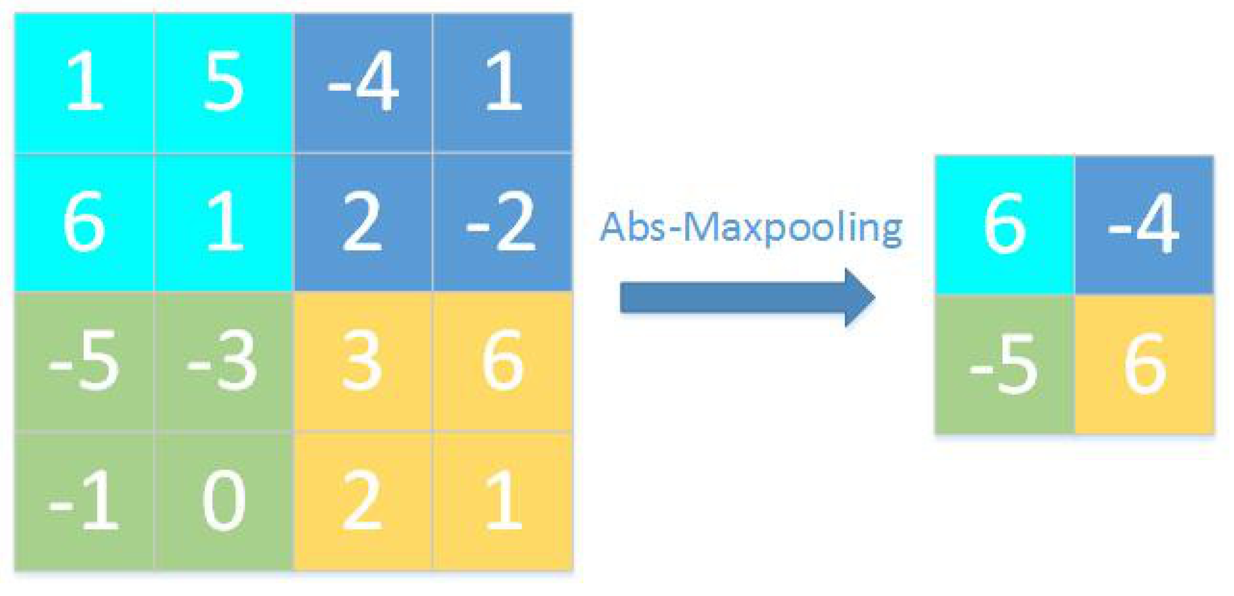
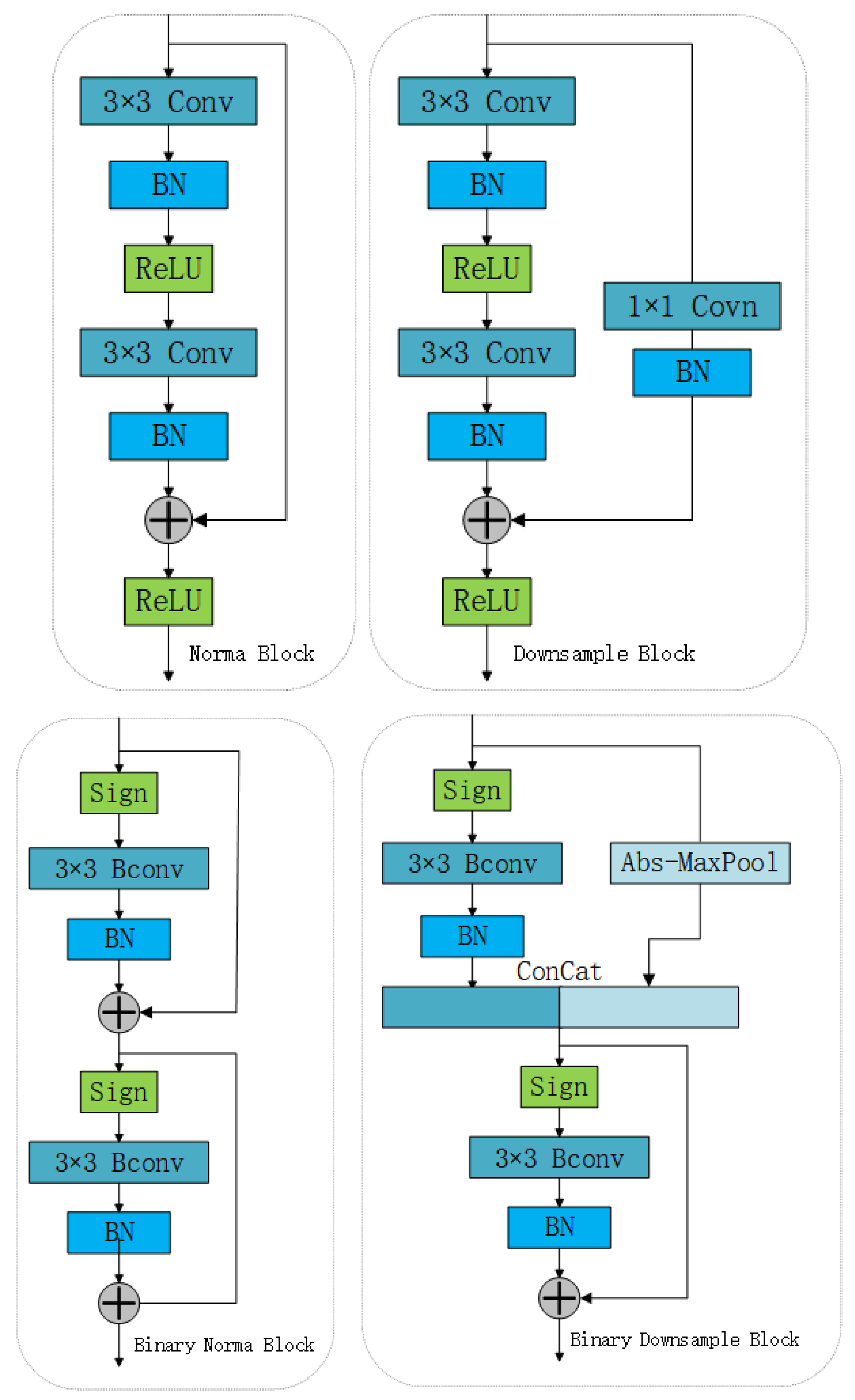
- Based on absolute value maximum pooling, we propose a downsampling method. The residual block of ResNet is adjusted and improved to make it more suitable for binary CNNs. In the pooling operation, the value with the largest absolute value in each pooling block is retained, and thus, the information of the feature map after binary quantization is retained more effectively. Such a downsampling layer does not require a full-precision convolution operation, which greatly reduces the number of floating-point operations used in the model.
- (2)
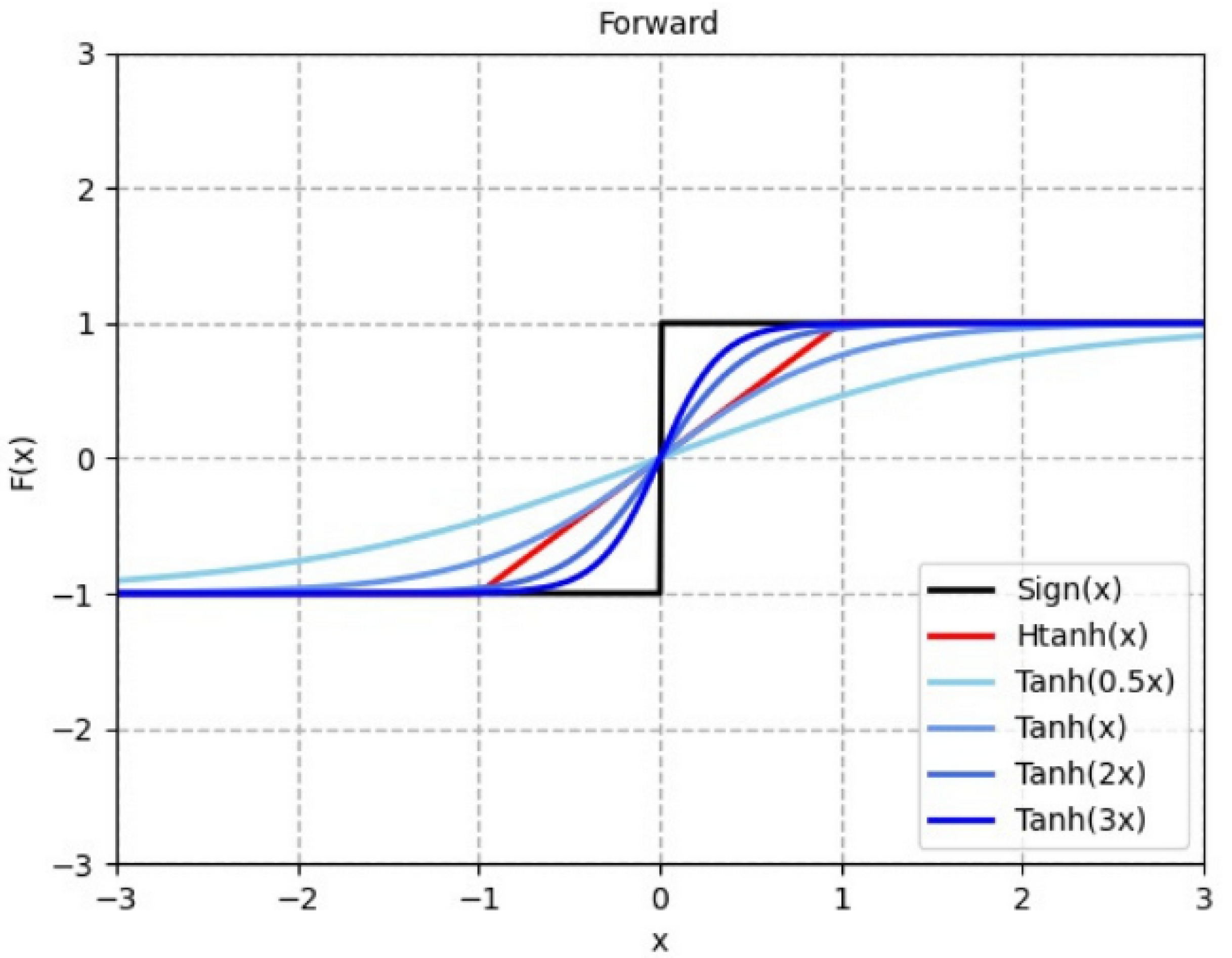
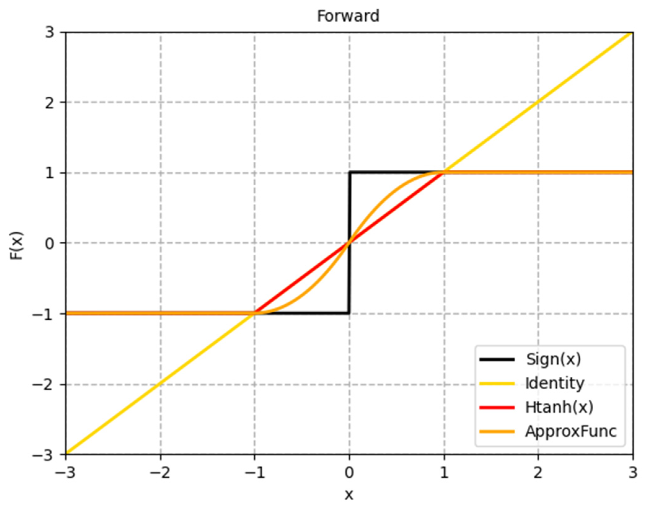
- For approximating the gradient of the symbolic function, a dynamic and progressive method is proposed that approximates the backpropagation gradient of the binarization function step-by-step during training. This method is used to more efficiently train the binarized CNN, addressing the problem that the model parameters cannot be updated in some intervals. The gradient of the later period gradually approaches the gradient of the symbolic function, considerably mitigating the gradient mismatch problem.
- (3)
- Herein, an information gain method is proposed, which is called the binarization of weight redistribution. The full-precision weights are standard deviation normalized before the weights are binarized. Floating-point gain terms that are introduced in most networks to reduce binary quantization errors are discarded, which enhances the information representation capability of the binary network and decreases the storage and operation burden of the traditional floating-point scaling gain.
2. Related Works
2.1. Binarized Convolutional Neural Networks
2.2. Vehicle Classification
2.3. Current Problems
- (1)
- In current approaches, to lighten the model by directly binarizing the full-precision network, the information flow is not sufficiently rich, and the use of 1 × 1 convolution for downsampling adds too many additional floating-point parameters and computations.
- (2)
- Existing approximation methods for symbolic functions of binarized networks ignore the problem that the parameters cannot be updated effectively in some cases, and there is a serious gradient mismatch problem.
- (3)
- The introduction of floating-point scaling in binarization networks to recover the weight quantization loss introduces additional floating-point parameters and computations, which increases the storage and operation burden of binarization CNNs.
3. Methods
3.1. Improved Binarized Residual Network
3.2. Binarization of Weight Redistribution
3.3. Dynamic Progressive Training
4. Experiments and Analysis of Results
4.1. Experimental Data Set and Experimental Parameters
4.2. Experimental Comparison and Analysis
4.3. Ablation Experiments
5. Conclusions and Future Work
Author Contributions
Funding
Data Availability Statement
Acknowledgments
Conflicts of Interest
References
- Simonyan, K.; Zisserman, A. Very deep convolutional networks for large-scale image recognition. arXiv 2014, arXiv:1409.1556. [Google Scholar]
- He, K.; Zhang, X.; Ren, S.; Sun, J. Deep residual learning for image recognition. In Proceedings of the IEEE Conference on Computer Vision and Pattern Recognition, Las Vegas, NV, USA, 26 June–1 July 2016; pp. 770–778. [Google Scholar]
- Courbariaux, M.; Bengio, Y. BinaryNet: Training Deep Neural Networks with Weights and Activations Constrained to +1 or −1. arXiv 2016, arXiv:1602.02830. [Google Scholar]
- Lin, X.; Zhao, C.; Pan, W. Towards accurate binary convolutional neural network. In Proceedings of the Advances in Neural Information Processing Systems, Long Beach, CA, USA, 4–7 December 2017. [Google Scholar]
- Tang, W.; Hua, G.; Wang, L. How to train a compact binary neural network with high accuracy? In Proceedings of the Thirty-First AAAI Conference on Artificial Intelligence, San Francisco, CA, USA, 4–9 February 2017. [Google Scholar]
- Darabi, S.; Belbahri, M.; Courbariaux, M.; Nia, V.P. BNN+: Improved binary network training. In Proceedings of the Sixth International Conference on Learning Representations, Vancouver, BC, Canada, 29 April–3 May 2018; pp. 1–10. [Google Scholar]
- Krizhevsky, A.; Hinton, G. Learning Multiple Layers of Features from Tiny Images; Technical Report TR-2009; University of Toronto: Toronto, ON, Canada, 2009. [Google Scholar]
- Dong, Z.; Wu, Y.; Pei, M.; Jia, Y. Vehicle type classification using a semisupervised convolutional neural network. IEEE Trans. Intell. Transp. Syst. 2015, 16, 2247–2256. [Google Scholar] [CrossRef]
- Rastegari, M.; Ordonez, V.; Redmon, J.; Farhadi, A. XNOR-Net: ImageNet classification using binary convolutional neural networks. In Proceedings of the European Conference on Computer Vision, Amsterdam, The Netherlands, 11–14 October 2016; pp. 525–542. [Google Scholar]
- Liu, Z.; Wu, B.; Luo, W.; Yang, X.; Liu, W.; Cheng, K.T. Bi-real Net: Enhancing the performance of 1-bit Cnns with improved representational capability and advanced training algorithm. In Proceedings of the European Conference on Computer Vision, Munich, Germany, 8–14 September 2018; pp. 722–737. [Google Scholar]
- Qin, H.; Gong, R.; Liu, X.; Shen, M.; Wei, Z.; Yu, F.; Song, J. Forward and backward information retention for accurate binary neural networks. In Proceedings of the IEEE Conference on Computer Vision and Pattern Recognition, Virtual. 14–19 June 2020; pp. 2250–2259. [Google Scholar]
- Liu, Z.; Shen, Z.; Savvides, M.; Cheng, K.T. ReActNet: Towards precise binary neural network with generalized activation functions. In Proceedings of the European Conference on Computer Vision, Virtual. 23–28 August 2020. [Google Scholar]
- Ding, R.; Liu, H.; Zhou, X. IE-Net: Information-Enhanced Binary Neural Networks for Accurate Classification. Electronics 2022, 11, 937. [Google Scholar] [CrossRef]
- Chen, P.Y.; Tang, C.H.; Chen, W.; Yu, H.-L. Dual path binary neural network. In Proceedings of the International SoC Design Conference (ISOCC), Jeju, Korea, 6–9 October 2019; pp. 251–252. [Google Scholar]
- Wang, P.; Cheng, Y.; Dong, B.; Gui, G. Binary Neural Networks for Wireless Interference Identification. IEEE Wirel. Commun. Lett. 2021, 11, 23–27. [Google Scholar] [CrossRef]
- Qian, Y.; Xiang, X. Binary neural networks for speech recognition. Front. Inf. Technol. Electron. Eng. 2019, 20, 701–715. [Google Scholar] [CrossRef]
- Jing, W.; Zhang, X.; Wang, J.; Di, D.; Chen, G.; Song, H. Binary Neural Network for Multispectral Image Classification. IEEE Geosci. Remote Sens. Lett. 2022, 19, 1–5. [Google Scholar] [CrossRef]
- Hasan, M.M.; Wang, Z.; Hussain, M.A.I.; Fatima, K. Bangladeshi Native Vehicle Classification Based on Transfer Learning with Deep Convolutional Neural Network. Sensors 2021, 21, 7545. [Google Scholar] [CrossRef] [PubMed]
- Habib, S.; Khan, N.F. An Optimized Approach to Vehicle-Type Classification Using a Convolutional Neural Network. CMC-Comput. Mater. Contin. 2021, 69, 3321–3335. [Google Scholar] [CrossRef]
- Chen, W.; Sun, Q.; Wang, J.; Dong, J.-J.; Xu, C. A novel model based on AdaBoost and deep CNN for vehicle classification. IEEE Access 2018, 6, 60445–60455. [Google Scholar] [CrossRef]
- Szegedy, C.; Liu, W.; Jia, Y.; Sermanet, P.; Reed, S.; Anguelov, D.; Erhan, D.; Vanhoucke, V.; Rabinovich, A. Going deeper with convolutions. In Proceedings of the IEEE Conference on Computer Vision and Pattern Recognition, Boston, MA, USA, 7–12 June 2015; pp. 1–9. [Google Scholar]
- Gong, R.; Liu, X.; Jiang, S.; Li, T.; Hu, P.; Lin, J.; Yu, F.; Yan, J. Differentiable soft quantization: Bridging full-precision and low-bit neural networks. In Proceedings of the IEEE International Conference on Computer Vision, Seoul, Korea, 27 October–2 November 2019; pp. 4852–4861. [Google Scholar]


| Item | Parameter |
|---|---|
| CPU | Intel Core i5-9400F 2.9 GHz x6 |
| GPU | NVIDIA GeForce RTX 2060 |
| Operating system | Ubuntu 16.04 LTS |
| Memory | 16 GB |
| Deep learning framework version | Pytorch 1.7.1 |
| Development languages | Python 3.6 |
| Downsampling Mode | Number of Participants | Floating-Point Multiplication Operands in Convolution | XNOR Operands in Convolution | |
|---|---|---|---|---|
| 32 bit | 1 bit | |||
| ResNet | 0 | 0 | ||
| Bi-Real-Net | ||||
| Ours | 0 | 0 | ||
| Model | Dataset | Binary Model | Weight/Activation (bit) | Accuracy (%) |
|---|---|---|---|---|
| ResNet-20 | CIFAR-10 | Full Precision | 32/32 | 91.2 |
| DSQ [22] | 1/1 | 84.1 | ||
| IR-Net | 1/1 | 86.8 | ||
| ReActNet | 1/1 | 85.8 | ||
| Ours | 1/1 | 86.3 |
| Dataset | Binary Model | Model Size (Mb) | Weight/Activation (bit) | Accuracy (%) |
|---|---|---|---|---|
| BIT-Vehicles | Full-Precision (ResNet-18) | 42.65 | 32/32 | 96.66 |
| BNN | 2.43 | 1/1 | 76.19 | |
| Bi-RealNet-18 | 9.20 | 1/1 | 89.60 | |
| XNOR-Net | 2.47 | 1/1 | 82.07 | |
| IR-Net (ResNet-18) | 2.05 | 1/1 | 92.33 | |
| Our model (ResNet-18) | 1.29 | 1/1 | 94.77 |
| Pooling Method | Accuracy (%) |
|---|---|
| AvgPooling | 93.92 |
| MaxPooling | 93.84 |
| Abs-MaxPooling | 94.77 |
| Experiment Number | Binarized Residual Block | Binarization of Weight Redistribution | Dynamic Progressive Training | Accuracy (%) |
|---|---|---|---|---|
| 1 | 82.51 | |||
| 2 | √ | 90.84 | ||
| 3 | √ | 92.64 | ||
| 4 | √ | 84.27 | ||
| 5 | √ | √ | 93.91 | |
| 6 | √ | √ | 93.89 | |
| 7 | √ | √ | 91.85 | |
| 8 | √ | √ | √ | 94.77 |
Publisher’s Note: MDPI stays neutral with regard to jurisdictional claims in published maps and institutional affiliations. |
© 2022 by the authors. Licensee MDPI, Basel, Switzerland. This article is an open access article distributed under the terms and conditions of the Creative Commons Attribution (CC BY) license (https://creativecommons.org/licenses/by/4.0/).
Share and Cite
Zhang, B.; Zeng, K. A Lightweight Method for Vehicle Classification Based on Improved Binarized Convolutional Neural Network. Electronics 2022, 11, 1852. https://doi.org/10.3390/electronics11121852
Zhang B, Zeng K. A Lightweight Method for Vehicle Classification Based on Improved Binarized Convolutional Neural Network. Electronics. 2022; 11(12):1852. https://doi.org/10.3390/electronics11121852
Chicago/Turabian StyleZhang, Bangyuan, and Kai Zeng. 2022. "A Lightweight Method for Vehicle Classification Based on Improved Binarized Convolutional Neural Network" Electronics 11, no. 12: 1852. https://doi.org/10.3390/electronics11121852
APA StyleZhang, B., & Zeng, K. (2022). A Lightweight Method for Vehicle Classification Based on Improved Binarized Convolutional Neural Network. Electronics, 11(12), 1852. https://doi.org/10.3390/electronics11121852