1. Introduction
With the increasing use of radio equipment, electronic countermeasures based on electronic reconnaissance are vital in modern warfare [
1,
2,
3]. According to the signal detection process of the electronic reconnaissance system, the radio frequency (RF) stealth [
4] of radiation sources mainly includes anti-interception [
5,
6,
7], anti-sorting [
8], and anti-identification. Due to the extensive applications of low SNR receivers and the rapid development of digital signal processing technology, radiation source anti-interception technology cannot be used to completely counter electronic reconnaissance from the enemy. Hence, it is critical for the anti-electronic reconnaissance system to weaken the sorting and identification abilities of the electronic reconnaissance system of the enemy [
9]. To obtain information about radiation sources in the environment, the electronic reconnaissance system sorting and identifying radiation source signal separates the pulse sequence of each radiation source from the random and staggered pulse stream received by the intercepted receiver [
10,
11]. The main sorting is the core of radiation source signal sorting, and the pulse repetition interval (PRI) and modulation mode of each radiation source in an electromagnetic environment are usually obtained by processing the arrival time of each pulse [
12,
13]. Therefore, it is necessary to combat PRI-based sorting to weaken the signal sorting and identification of the electronic reconnaissance system of the enemy. We will study the sorting algorithm in the sorting field and the countermeasures against PRI-based sorting in order to weaken the signal sorting and to identify the electronic reconnaissance system of the enemy.
At present, the field of signal sorting mainly focuses on the improvement of the signal sorting algorithm and the design of the anti-PRI sorting method. On the one hand, the signal sorting algorithm mainly puts forward the corresponding improved SDIF algorithm based on SDIF for different signal sorting failure situations. The literature [
14] points out that because time of arrival (TOA) is easily affected by the jitter of PRI, the SDIF algorithm cannot effectively sort the PRI jitter signal. Therefore, an improved algorithm is proposed based on the SDIF algorithm. The sorting efficiency of the algorithm for jitter signals is notably improved by using overlapping PRI bins. Furthermore, the search speed is also improved. In reference [
15], an improved SDIF algorithm was proposed to solve the problem of “increasing batch” in the signal sorting of multi-function radars (MFRs) with various work modes. The improved method utilizes a limited penetrable visibility graph to construct the network from interleaved radar pulse sequences and then employs a label propagation algorithm and density peak clustering to detect community structures, thus fulfilling the deinterleaving of pulses from several MFRs. The above methods can effectively solve the problem of increasing batch in the process of sorting. The authors in [
16] compared several commonly used sorting algorithms and obtained an optimal sorting algorithm under different circumstances. With the extensive application of radio equipment, a single sorting algorithm is not enough to sort high density pulse current in complex electromagnetic environments. Therefore, the authors in [
17] comprehensively used the PRI transform and SDIF algorithm to sort signals, achieving good sorting effects for all kinds of signals. The authors in [
18] comprehensively applied clustering and SDIF sorting methods to improve the sorting speed and accuracy and meet the real-time requirements of sorting. The above is a brief introduction to the development of the signal sorting algorithm. The above literature mainly focuses on the failure of the SDIF sorting algorithm caused by different signal sorting situations. Then SDIF is analyzed. Finally, improved sorting algorithms based on the SDIF algorithm are obtained. However, starting with the work flow of the SDIF algorithm, this paper studies the failure principle of the threshold function in the SDIF algorithm in order to provide theoretical support for anti-sorting signal design. On the other hand, the research on anti-PRI sorting mainly focuses on the design technology of anti-sorting signals. There are three design methods for anti-sorting signals. Firstly, jamming pulses are added to the radar signal to disrupt the interception and recognition of the PRI pulse signal by the enemy interception receiver [
19,
20,
21,
22]. Then, jitter is added to the PRI of the pulse signal, and every pulse has a different PRI. Thus, it is difficult for the enemy intercepting receiver to sort the radar signal [
21,
23,
24]. At last, the PRI of the pulse or signal system is optimized, and the accurate and quantitative design of the PRI is required only, without the additional design of interference pulses [
25,
26]. Although the above methods have achieved a certain effect, the stability of the anti-sorting performance of the designed signal needs to be further verified. The method of signal design relies more on the experience of researchers and lacks the strict sorting failure principle as a theoretical guide.
The failure mechanism of the classical sequential difference histogram (SDIF) in the PRI sorting algorithm is studied in this paper to establish a theoretical basis for the design of an anti-PRI sorting signal. It is proposed for the first time that the SDIF algorithm threshold function will fail when the signal PRI values obey the interval distribution whose length is more than 20 times of the minimum interval PRI, as will be proved by formula derivation. The rest of this paper is organized as follows:
Section 2 analyzes the SDIF sorting algorithm in detail.
Section 3 discusses the failure principle of SDIF sorting; the signal parameters are designed according to the sorting failure principle, and the designed signal is simultaneously verified by the simulation and experiment in
Section 4. In
Section 5, the full paper is summarized.
2. Sequential Difference Histogram (SDIF)
Radar signal source sorting is also known as deinterleaving of the radar radiation source signal. It refers to the process of separating radar pulse trains from random and staggered pulse streams. In essence, it is the parameter matching of each signal pulse. Researchers treat the most similar pulses as pulse sequences produced by the same signal source using characteristic parameters extracted in different domains or measured between or within pulses and matching with them in the databases or each other. Otherwise, they are regarded as pulses generated by various radiation sources to complete the de-interlacing of the pulse flow.
In engineering, histogram sorting is the most commonly-used method to estimate the PRI value of the radiation source signal based on statistical principles. After the difference of time of arrival (TOA) is counted, the histogram of the difference is formed. Then, the appropriate sorting threshold and sorting strategy are set. In the 1980s, the most traditional histogram sorting algorithm could be used to calculate the TOA difference of any two pulses, and the histogram of all TOA differences was formed. The PRI estimate can be obtained by comparing each histogram with the threshold function. The traditional histogram sorting method contains all the information of the pulse flow. Thus, it is insusceptible to pulse loss and other adverse effects. However, this method is time-consuming, with a large calculation amount and a lack of real-time performance. Therefore, researchers improved the traditional histogram method. The Cumulative Difference Histogram (CDIF) and Sequential Difference Histogram (SDIF) are two improved algorithms commonly used in engineering.
In essence, both SDIF and CDIF belong to TOA difference histogram sorting methods [
27,
28]. The TOA difference of pulses is counted by the two sorting algorithms according to certain rules, and PRI estimation is analyzed. Then, the impulse train search is performed based on the PRI estimate. At last, the radiation source pulse trains are extracted. Compared with the traditional histogram sorting algorithm, SDIF and CDIF algorithms greatly reduce the computational amount and are real-time. SDIF and CDIF algorithms can sort PRI fixed, PRI stagger, and jitter radiation source signals and are widely used in the engineering field [
29,
30,
31].
Compared with the CDIF algorithm, the SDIF algorithm has the following advantages: SDIF only analyzes the histograms of the current level without the histogram statistics of different levels and the 2× PRI test. It requires less computation and has a faster processing speed. In addition, the SDIF algorithm has an optimized threshold function. In combination with sub-harmonic detection, false detection is avoided in the SDIF algorithm. Therefore, SDIF is more widely used than is CDIF. In this paper, the failure mechanism of the SDIF algorithm is mainly studied. SDIF algorithm flows are as follows.
According to Algorithm 1, the SDIF histogram mainly includes two parts: TOA difference histogram analysis, and impulse sequence search. TOA difference histogram analysis is mainly used to estimate PRI values. The histogram statistics method is used to calculate the number of TOA differences from level one to a higher level. If the number of TOA difference statistics exceeds the detection threshold, the TOA difference corresponding to the peak divided by the statistical series of the TOA difference is the possible PRI value.
| Algorithm 1 Deinterleaving signal via SDIF |
| Input: Time of arrival (TOA) |
| Initialization: difference level C |
| 1: Judge the TOA number of level C |
| 2: Calculate the TOA difference of level C |
| 3: Count the TOA difference of level C and form a histogram |
| 4: Determine the detection threshold and obtain the PRI estimation |
| 5: Subharmonic check |
| 6: Determine the unique PRI estimate |
| 7: Sequence search |
| 8: Removes the searched pulse train from the pulse stream |
| 9: The remaining pulses are sorted until the number of pulses is less than 5 or the number of PRI in the first-level histogram exceeding the threshold is not unique |
| 10: Increase difference level C and repeat the above steps until the sorting is over |
Therefore, it is essential to determine the threshold formula. In the analysis of the entire signal intercept, the TOA difference between two adjacent pulses approximates a random event because of the receiver obtaining signals from multiple sources during the sampling time of the SDIF histogram. Hence, the TOA distribution of each pulse approximates the Poisson distribution. It can be expressed as:
where
is the average number of signal pulses reaching the intercepted receiver per unit time;
x indicates the actual arrival number of signal pulses per unit time. Then, the probability that there are
w pulses in the time interval
, namely
x =
w, can be expressed as:
where
b is the pulse current density,
and
n is the total number of pulses, and T is pulse duration. According to the meanings of parameters in (1) and (2), we get
in (2). If
is the time interval between adjacent pulses, namely, having zero pulses in the time interval (
w = 0), the probability is
In the level c histogram, there are
E −
C time intervals if the number of pulses is
E. The parameter of the Poisson process is
[
28]. We can conclude that the optimal function of the detection threshold is expressed as:
where
E is the total number of pulses;
C is the order of the histogram;
k is a positive constant less than 1;
N is the total number of bins in the histogram. The optimum values of the constants
a and
k are experimentally determined. According to mathematics, a function graph of a dependent variable that changes with an independent variable is given in
Figure 1, in which the threshold function is a monotonically decreasing exponential function with the signal PRI value as an independent variable.
In the actual signal sorting process of the SDIF sorting algorithm, we need to avoid the influence of the intercept receiver on the pulse TOA measurement and enhance the sorting performance of the algorithm for jitter signals. Therefore, the tolerance
of signal PRI value
is set in SDIF and its improved sorting algorithm. The interval
is determined by the tolerance, namely, the PRI interval or a small box of PRI. The upper and lower limits of the small box can be expressed as:
Then the box range of PRI value is
. The PRI value of the histogram is the weighted average of the values that fall into the PRI box. Hence, the weighted average function should be:
where
S is the sum of the pulse number corresponding to adjacent PRI values
within the tolerance;
is the number of PRI values
corresponding to pulses within tolerance.
The above is a detailed description of the PRI estimates in the first step. Then, the signal sequence search in the second step of the algorithm is analyzed. The sequence search extracts the radiation source pulse train from the PRI estimate obtained in the first step. In the first place, the PRI estimation is used to judge whether three pulses can be continuously searched in the staggered pulse stream. If it is useful, it is true PRI. Then, the remaining pulses of the radiation source whose arrival time difference is close to each other are searched backward successively, with these three pulses as the starting point. If it is useless, it is false PRI, and the PRI estimation is discarded. In addition, we can use other PRI estimates that exceed the threshold of the sequence search. The estimated PRI obtained in the first step can also be screened, and the real value of PRI can be obtained via the pulse sequence search.
3. SDIF Sorting Failure Principle
According to the analysis in the previous section, SDIF sorting is based on the estimation of the PRI value in the first step. The important step to determine whether the PRI value can be used as the PRI estimate of the sorting algorithm is to compare the pulse number of histogram statistics with the pulse number threshold of the sorting algorithm. If the pulse number counted by the histogram exceeds the threshold value, the sorting algorithm is a possible PRI estimate. Then, we can check the sub-harmonics and enter other subsequent stages. In contrast, if the pulse number counted by the histogram is less than the threshold, it is not a possible PRI estimation.
Induction and proofs are mainly used in this paper. Firstly, the accuracy of the SDIF sorting algorithm for fixed PRI is verified by the special case level histogram of signal sorting. Then, signal PRI values increase from one fixed value to two or more when the total number of pulses is constant. In addition, the PRI critical condition that invalidates the sorting algorithm is proved correct. Thirdly, the sorting results of the algorithm are discussed when signal PRI values obey the interval distribution. At last, the sorting results of the signal PRI obeying the interval distribution by a multistage histogram are discussed. The logic diagram of the derived SDIF separation failure principle is given in
Figure 2.
3.1. Analysis of Sorting Failure Principle of the First-Order Histogram
When the signal is a fixed-period signal, namely, , we assume that the number of pulses E is ; and a are the positive constant less than 1 when in the threshold Formula (4). The number of pulses is in the actual situation. Therefore, the right part of the threshold formula is , and the threshold formula is when . The signal PRI value can be sorted out.
3.1.1. The Number of PRI Values Increases from One to a Finite Number
The number of PRI values increases from 1 to 2, assuming the total number of pulses is constant, which means the signals are two stagger signals. In addition, the value of PRI is or (). There are pulses in each value of PRI. The relationship between the number of corresponding pulses and the threshold value is discussed when the PRI value and pulse number have changed.
According to Formula (4), when the PRI value is
, the threshold of the algorithm should be:
When the PRI value is
, the threshold of the algorithm can be expressed as
When the threshold of the algorithm is
, namely,
, the PRI critical value of sorting failure can be calculated by Formula (10).
represents the total number of pulses, which is usually in the tens of thousands, namely,
. Therefore, Equation (10) can be simplified as:
Therefore, after taking the natural logarithm of the above formula, we can obtain
:
With the monotonically decreasing property of the threshold function, it can be known that:
The SDIF algorithm can sort out the pulses of PRI when , namely, . The SDIF algorithm can also sort out the pulses of PRI due to . The SDIF algorithm cannot sort out the pulses of PRI when . However, if , the SDIF algorithm can sort out the pulses of PRI , and if , the SDIF algorithm cannot sort out them. Consequently, the SDIF algorithm cannot sort the signal pulse whose PRI is less than the critical value when the number of PRI values increases from 1 to 2.
According to the above analysis, the actual signal sorting situation is extended, and the derivation condition is assumed as follows:
- (1)
The total number of pulses is still .
- (2)
The number of the PRI value increases to a limited number, which means the signals are multiple stagger signals.
- (3)
The values of PRI are , ().
- (4)
The number of pulses corresponding to each PRI value is .
The derivation process is the same as that of Equations (8)–(12). Hence, we will not repeat it here. The PRI critical value of sorting failure is solved as:
At last, the SDIF algorithm cannot select the signal pulse whose PRI is less than the critical value when the number of PRI signals increases to a finite number.
3.1.2. The Signal PRI Value Follows an Interval Distribution
We assume that the number of pulses
E is
. The signal PRI value follows an interval distribution
. The design of transmitting signals and the processing of echo signals need to be considered in the radar field. Hence, the PRI value of the radar signal does not obey completely random disordered distribution. Thus, the PRI values of signals are discussed with uniform distribution in this section. For any given interval, the number of pulses
is:
where
is the total number of pulses,
and
are the maximum and minimum values of the distribution interval, respectively, and
z is the minimum interval of PRI values within the interval distribution. When PRI is
, the threshold calculation formula of the algorithm is shown in Equation (4).
When
,
where
is the total number of pulses,
. Therefore, the above formula can be simplified as:
Thus, the PRI critical value of sorting failure is solved as:
When , the number of pulses corresponding to PRI values in the interval is less than the threshold value. Hence, the SDIF algorithm sorting fails. When , the number of pulses corresponding to the PRI value in interval is less than the threshold value. Thus, SDIF algorithm sorting also fails in the interval . The number of pulses corresponding to the PRI value in the interval is larger than the threshold value. The signal can be sorted successfully. When the PRI value of the signal follows the interval distribution, the SDIF algorithm cannot select the signal pulse whose PRI is less than the critical value .
The conditions in the actual signal sorting process are described as follows:
- (1)
N is the number of cells counted in the histogram and is usually above 1000.
- (2)
z is the minimum interval of PRI. In general, z, , and have the same size scale, all of which are in the microsecond level.
- (3)
a, k in Equation (4).
Therefore, when the interval length is 20 times larger than z, we can know that . Thus, the threshold value is much larger than any value in the interval , namely, .
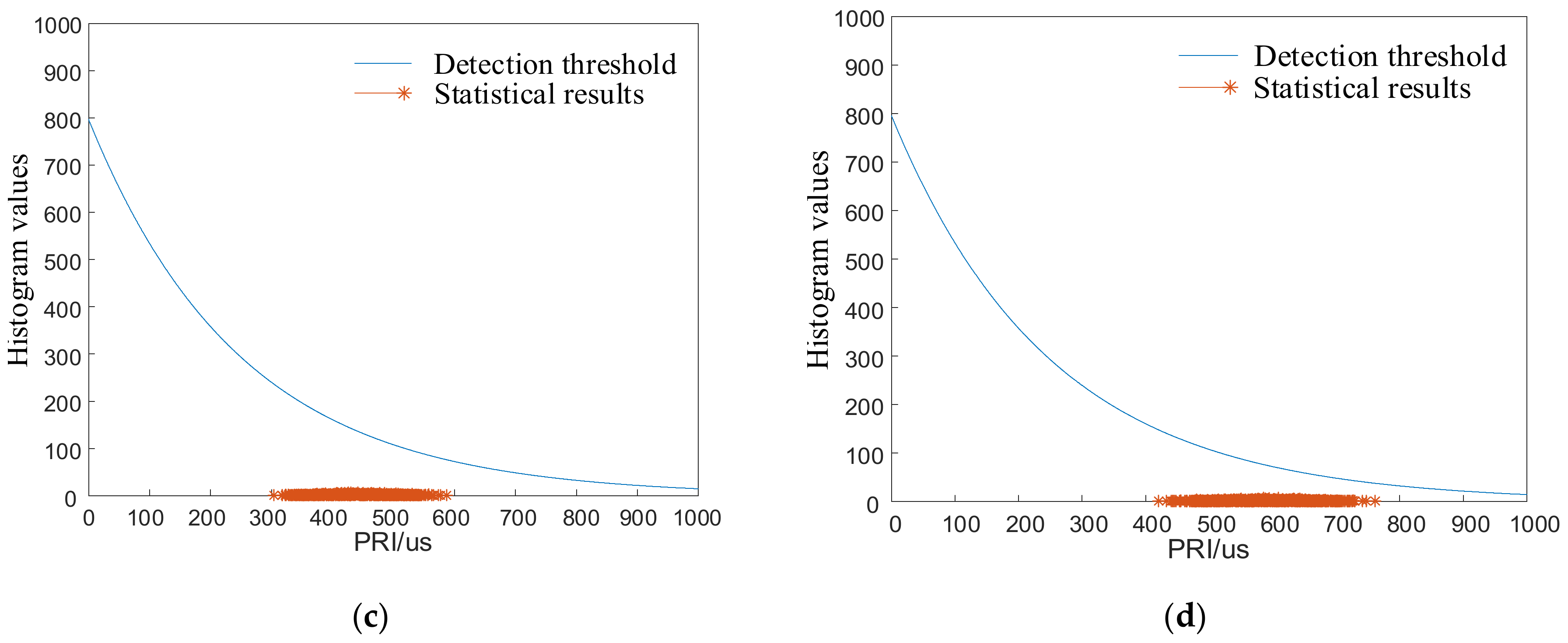
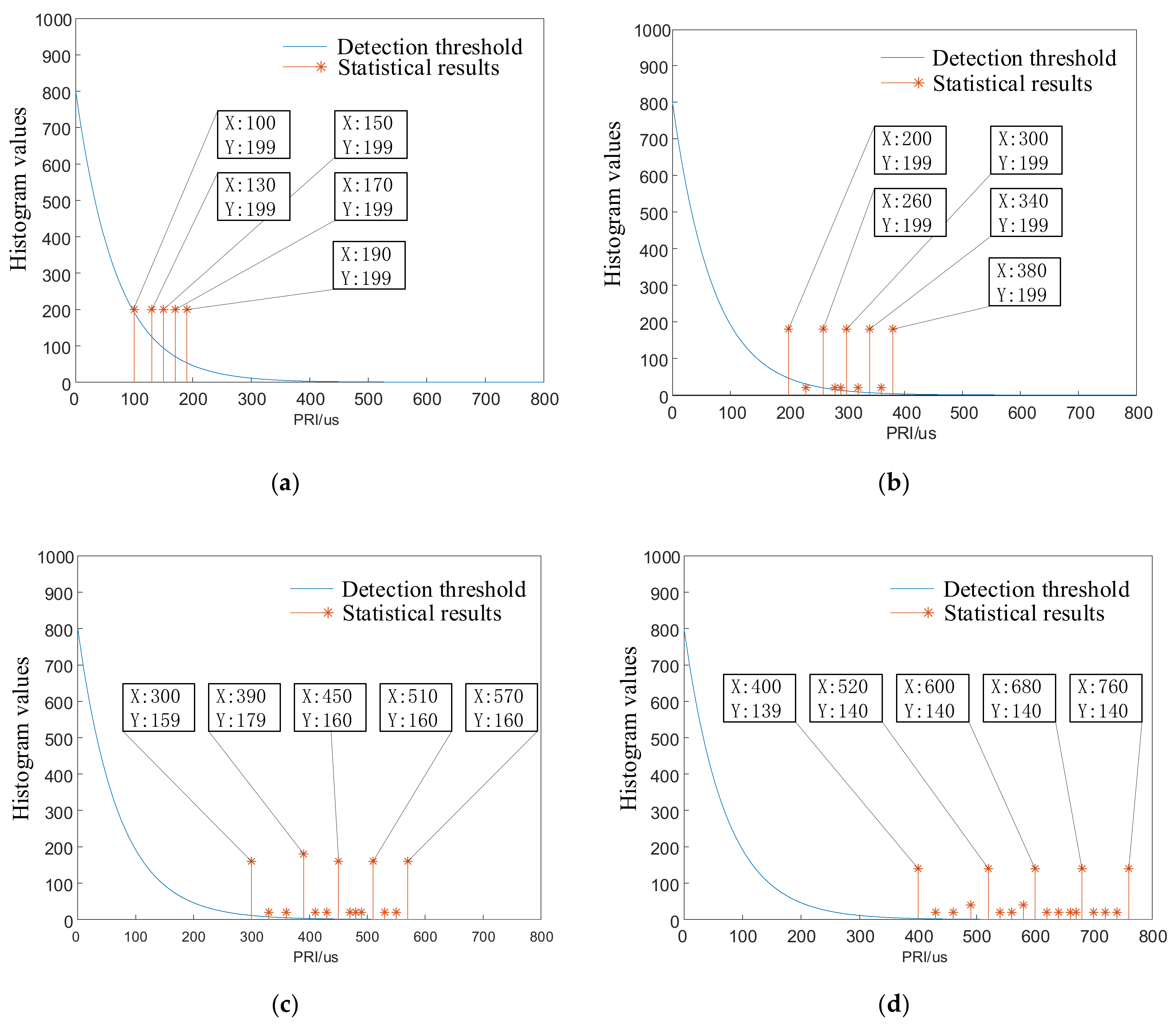
In conclusion, when signal PRI values obey the interval distribution, and the interval length is 20 times larger than z, the number of pulses corresponding to any PRI value in the interval is less than the threshold value of the sorting algorithm in the analysis of the sorting failure principle of the first-order histogram. Hence, the SDIF algorithm fails in signal sorting.
3.2. Analysis of Sorting Failure Principle in Multi-Order Histogram
Sometimes, the SDIF sorting algorithm has multiple PRI values exceeding the threshold in the first-order histogram. We must count the secondary, tertiary, and advanced histograms to produce PRI estimates. Therefore, it is also necessary to analyze the sorting failure principle of the histograms from secondary to advanced.
We assume that the number of pulses
E is
. The signal PRI value follows an interval distribution
. Because the design of the transmitting signal and processing of the echo signal need to be considered together in the radar field, the PRI value of the radar signal will not be a completely random and disordered distribution. Hence, the PRI values of signals are discussed with a uniform distribution in this section. For any given interval, the number of pulses
is:
where
is the total number of pulses,
and
are the maximum and minimum values of the distribution interval, respectively, and
z is the minimum interval of PRI values within the interval distribution. When the value of PRI is
, the threshold calculation formula of the algorithm is shown in Equation (4).
When
:
where
represents the total number of pulses, and
C represents the histogram sorting series. In the actual sorting process,
, although
. Equation (19) is simplified to:
Thus, the PRI critical value of sorting failure is solved as:
The PRI values distribution and signal sorting results are shown in
Table 1.
The conditions in the actual signal sorting process are described as follows:
- (1)
N is the number of cells counted in the histogram and is usually above 1000.
- (2)
z is the minimum interval of PRI. In general, z, , and have the same size scale, all of which are in the microsecond level.
- (3)
a, k in Equation (4).
Therefore, when the interval length is 20 times larger than z, we can know that . Thus, the threshold value is much larger than any value in the interval , namely, .
In conclusion, when signal PRI values obey the interval distribution, and the interval length is 20 times larger than z, the number of pulses corresponding to any PRI value in the interval is less than the threshold value of the sorting algorithm in the analysis of the sorting failure principle of the high-order histogram. Hence, the SDIF algorithm fails in signal sorting.


