Complex Permittivity Measurement of Low-Loss Anisotropic Dielectric Materials at Hundreds of Megahertz

Abstract

Resonant methods are well known for their accuracy in determining the complex permittivity of materials. However, to guarantee the accuracy, interference modes must be suppressed in the measurement band. In this paper, a multi-mode split rectangular cavity is designed and fabricated to measure low-loss anisotropic dielectric materials in the frequency range from 300 to 1000 MHz. Details of the cavity design are presented. Simulation results for a uniaxially anisotropic material validate both the setup and the processing. Moreover, validation measurements on a sheet of polytetrafluoroethylene (PTFE) are in agreement with the literature data, which indicate that the proposed method in this paper is reliable and accurate for low-loss complex permittivity characterization at hundreds of megahertz.

1. Introduction

Measurement of electromagnetic parameters of materials, such as relative complex permittivity, is important in understanding their behavior in response to applied electromagnetic fields [1]. The knowledge of the complex permittivity values of materials is a prerequisite step for many types of electromagnetic applications. A wide variety of high-frequency methods for measuring the permittivity and loss tangent of dielectric materials is described in the literature. The methods are divided into two categories: non-resonant and resonant [2,3].

Non-resonant methods are mostly based on measurements of transmitted and/or reflected electromagnetic power from a sample under test illuminated by a well-determined incident electromagnetic wave. Methods using transmission-line approaches have been developed using a coaxal cell [4,5], a rectangular waveguide [6,7,8], a partially filled waveguide [9,10,11], a coplanar waveguide [12], or a flat sample in free space [13,14,15,16,17]. Determining complex permittivity from far-field scattering patterns is another type of non-resonant method [18,19].

Resonant-type methods measure electromagnetic parameters by using a change in resonant frequency and quality factor after the sample is inserted into the measurement cell. Generally speaking, resonance methods provide the best accuracy in the estimation of both real and imaginary parts of permittivity for low-loss dielectrics. The methods include different types of resonant cavities loaded with the material under test, such as TE_01n mode cylindrical cavity [20,21], TM_0n0 mode cylindrical cavity [22,23], rectangular cavity [24,25], Fabry–Perot resonator [26,27], etc. The sample under test can also create a dielectric resonator in the modes of TE₀₁₁ mode [28,29], TE_01δ mode [30,31], and whispering gallery mode [32,33], etc.

The complex permittivity of an isotropic material can be written as

$$\epsilon ={\epsilon }_0{\epsilon }_{\mathrm{r}}={\epsilon }_0{{\epsilon }^{\prime }}_{\mathrm{r}}\left(1-\mathrm{j}\tan \delta \right)$$

(1)

where ${\epsilon }_{\mathrm{r}}$ is the relative complex permittivity, $\tan \delta$ is the loss tangent, and ${\epsilon }_0\approx 8.8542\times {10}^{-12} \mathrm{F}/\mathrm{m}$ denotes permittivity of the vacuum. In general, the permittivity of any linear material is defined as a tensor quantity that describes the relationship between the electric displacement D and the electric field E vectors

$$D=\overline{\overline{\epsilon }}E$$

(2)

The permittivity tensor of uniaxially anisotropic materials can be written as

$$\overline{\overline{\epsilon }}={\epsilon }_0\left[\begin{array}{ccc}{\epsilon }_{r\parallel }& 0& 0\\ 0& {\epsilon }_{r\perp }& 0\\ 0& 0& {\epsilon }_{r\perp }\end{array}\right]$$

(3)

where $\parallel$ and $\perp$ represent the parallel and perpendicular components, respectively.

If samples under test are anisotropic, they must be oriented and cut with respect to their anisotropy axis. Some ingenious methods have been developed to measure the permittivity tensor of anisotropic materials. These methods also fall into non-resonant methods and resonant methods. Non-resonant methods for measuring the permittivity tensor of materials generally operate by placing a sample in a section of transmission line and measuring the two-port scattering parameters with the sample oriented parallelly and perpendicularly to the transverse electric field component of the propagating wave [34,35,36,37]. There are also some successful examples in the resonant methods to measure the permittivity tensor, such as the dielectric resonator method [38,39,40] and the dielectric-loaded metal cavity method [41,42,43].

The aim of this study is to present a technique to measure the complex permittivity of low-loss uniaxially anisotropic materials at hundreds of megahertz. Measurements on low-loss materials at GHz frequencies are typically performed in cylindrical cavities, whereas, at hundreds of megahertz, the large size of cylindrical cavities is a practical limitation. Therefore, it is possible to use rectangular cavities for they can be made of flat plates.

The remaining parts are organized as follows. In Section 2, a multi-mode rectangular cavity is designed for measuring uniaxially anisotropic materials at six frequencies from 300 MHz to 1000 MHz. In addition, a perturbation method and a rigorous iterative method are given to determine the complex permittivity. The simulation and the measurement results are provided in Section 3 and Section 4, respectively. The last part, Section 5, concludes this work.

2. Theory

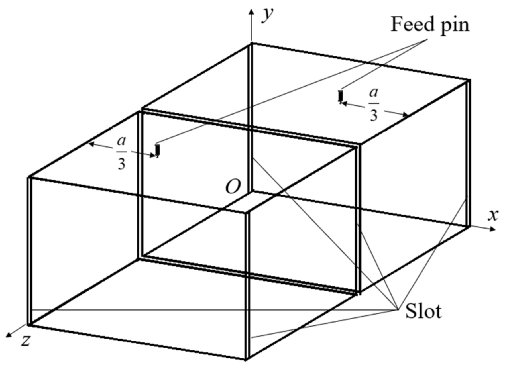
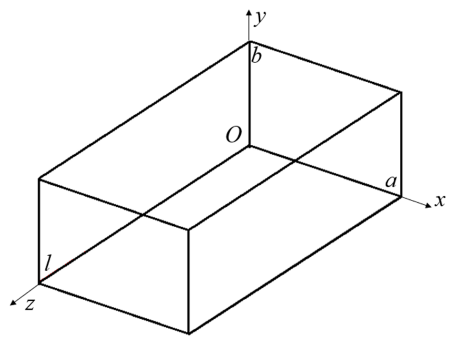
2.1. Rectangular Cavity Design

The geometry of a rectangular cavity is shown in Figure 1. It consists of a length l of rectangular waveguide shorted at both ends. The side lengths of the cross section of the waveguide are a and b. Under the assumption that the cavity is lossless, applying the condition that tangent electric vanishes on the conducting walls gives the resonant frequency of the TE_mnp or TM_mnp mode by

$$f_{mnp}=\frac{c}{2\pi }\sqrt{{\left(\frac{m\pi }{a}\right)}^2+{\left(\frac{n\pi }{b}\right)}^2+{\left(\frac{p\pi }{l}\right)}^2}$$

(4)

where the indices m, n, and p refer to the number of variations in the standing wave pattern in the x, y, and z directions.

In Figure 1, the z axis is parallel with the side l. Therefore, the resonant frequency calculated by (1) is of TE^l_mnp or TM^l_mnp mode. If the z axis is parallel with the side a or b, there are four more groups of modes like TE^a_mnp, TM^a_mnp, TE^b_mnp, and TM^b_mnp. In this paper, to measure the tensor permittivity at several frequencies in a split rectangular cavity, six modes are employed, which are TE^l₁₀₁, TE^l₁₀₃, TE^l₁₀₅, TE^l₂₀₁, TE^l₂₀₃, and TE^l₂₀₅ modes. Since the second index n is zero, the resonant frequencies of these modes are independent with the length of b. To make the six frequencies distribute from 300 MHz to 1000 MHz as evenly as possible, the a and l are chosen as

$$\begin{array}{c}a=488\mathrm{mm}\\ l=951\mathrm{mm}\end{array}$$

(5)

The resonant frequencies of six measurement modes are shown in Figure 2, as well as resonant frequencies below 1100 MHz of other modes calculated by (4). In Figure 2, b is chosen the same as a. It can be seen in Figure 2 that there are excessive amounts of interference modes in the cavity, and many of them are degenerated. It is unpractical to distinguish the wanted modes from them.

Since the split rectangular cavity is used, there is a slot in the middle of the cavity, shown in Figure 3. Due to the fact that the modes with the electric current perpendicular to the slot are radiating, the resonant of these modes are negligible. They are TE^l_mnp and TM^l_mnp modes with even number p, TE^a_mnp modes with even number m, and TE^b_mnp and TM^b_mnp modes with even number n.

There are still a large number of interference modes left in the split rectangular cavity with a split in the middle. Extra work needs to be conducted to reduce the unwanted modes. If the feeding pins are at x = a/3, shown in Figure 3, due to the electric field distribution, more modes are suppressed. The suppressed modes are TE^l_mnp and TM^l_mnp modes with divisible-by-three m, TE^a_mnp and TM^a_mnp modes with divisible-by-three p, TM^b_mnp modes with divisible-by-three n, and all TE^b_mnp modes.

Four extra slots along y-axis are introduced at the corners of the cavity to suppress more modes. The modes with electric current perpendicular to these slots are prone to be radiated through these slots. As a result of that, a large number of modes are suppressed. They are TE^l_mnp and TE^a_mnp modes with greater-than-zero n, and all TM^l_mnp and TM^a_mnp modes.

With the above efforts, the only interference modes left are TM^b_mnp modes with odd-number n, not-divisible-by-three m, and greater-than-0 p. If a small length of b is chosen, all the resonant frequencies of the interference modes are outside the measurement band, while the resonant frequencies of the TE^l_10p and TE^l_20p modes do not change. However, small b implies a low-quality factor. Therefore, b is chosen so that some interference modes are in the measurement band but are far from the measurement modes. The chosen b is

$$b=309\mathrm{mm}$$

(6)

Figure 4 shows the resonant frequencies of the measurement modes and interference modes of the cavity illustrated in Figure 3 with the size given by (5) and (6).

2.2. Complex Permittivity Determination by Perturbation Method

The total fields for the TE^l_m0p mode can be written as

$$\begin{array}{l}{E}_x=0\\ E_y=\frac{\omega {\mu }_{0}m\pi }{k_c^{2}a}\sin \frac{m\pi x}{a}\sin \frac{p\pi z}{l}\\ E_z=0\\ H_x=-\frac{\mathrm{j}pm{\pi }^2}{k_c^{2}al}\sin \frac{m\pi x}{a}\cos \frac{p\pi z}{l}\\ H_y=0\\ H_z=\mathrm{j}\cos \frac{m\pi x}{a}\sin \frac{p\pi z}{l}\end{array}$$

(7)

The power loss in the conducting walls is given as

$$P_c=\frac{R_s}{2}{\displaystyle \underset{}{∯}{H}_t{}^2\mathrm{d}s}=\sqrt{\frac{\omega {\mu }_0}{2\sigma }}\left[\frac{p^2{m}^2{\pi }^{4}ab}{2k_c^4{a}^2{l}^2}+\frac{p^2{m}^2{\pi }^4}{4k_c^{4}al}+\frac{al}{4}+\frac{bl}{2}\right]$$

(8)

where, R_s is the surface resistivity of the metallic walls, σ is the conductivity of the metallic walls, H_t is the tangential magnetic field at the surface of the walls, k_c = mπ/a is the cutoff wavenumber. The total stored energy is

$$W=\frac{{\epsilon }_0}{2}{\displaystyle {\int }_0^a{\displaystyle {\int }_0^b{\displaystyle {\int }_0^l{\left|E_y\right|}^2\mathrm{d}x\mathrm{d}y\mathrm{d}z}}}=\frac{{\epsilon }_0{\omega }^2{\mu }_0{}^2{m}^2{\pi }^{2}bl}{8k_c^{4}a}$$

(9)

Then, the conductor quality factor Q_c of the cavity with lossy conducting walls and lossless dielectric can be found as

$$Q_c=\frac{\omega W}{P_c}=\frac{{\epsilon }_0{\omega }^3{\mu }_0{}^2{m}^2{\pi }^{2}bl}{8R_s{k}_c^{4}a\left[\frac{p^2{m}^2{\pi }^{4}b}{2k_c^{4}a{l}^2}+\frac{p^2{m}^2{\pi }^4}{4k_c^{4}al}+\frac{al}{4}+\frac{bl}{2}\right]}$$

(10)

If the cavity is perturbed by the insertion of a thin dielectric slab into the middle slot, as shown in Figure 5, the resonant frequency changes. The perturbation method assumes that actual fields with a small perturbation are not greatly different from those of the unperturbed cavity. From the perturbation method, we have

$$\frac{f_0-f}{f_0}=\frac{\left({\epsilon }_r-1\right){\epsilon }_{0}t{\displaystyle {\int }_0^a{\displaystyle {\int }_0^b{\left|E_0\right|}^2\mathrm{d}x\mathrm{d}y}}}{4W}$$

(11)

where, ε_r and t are the permittivity and thickness of the inserted thin dielectric slab, respectively; E₀ and W are the unperturbed field and total stored energy, respectively; and f₀ and f are the unperturbed and perturbed resonant frequency, respectively. Using (7) and (9) in (11) gives

$${\epsilon }_r=\frac{\left(f_0-f\right)l}{f_{0}t}+1$$

(12)

With the perturbation, the total quality factor Q₀ is reduced due to the dielectric loss, and becomes the loaded quality factor Q_L. The power dissipated in the dielectric is

$$P_d=\frac{\omega {\epsilon }_r{\epsilon }_0\tan \delta }{2}t{\displaystyle {\int }_0^a{\displaystyle {\int }_0^b{\left|E_0\right|}^2\mathrm{d}x\mathrm{d}y}}=\frac{{\omega }^3{\epsilon }_r{\epsilon }_0{\mu }_0{}^2{m}^2{\pi }^{2}bt\tan \delta }{4k_c^{4}a}$$

(13)

The perturbation method also assumes that the Q_c of the cavity does not change. Therefore, we have

$$\frac{1}{Q_L}=\frac{1}{Q_c}+\frac{1}{Q_d}$$

(14)

where, Q_c is the same as (10). The dielectric quality factor Q_d is

$$Q_d=\frac{\omega W}{P_d}=\frac{l}{2{\epsilon }_{r}t\tan \delta }$$

(15)

2.3. Rigorous Iterative Complex Permittivity Determination

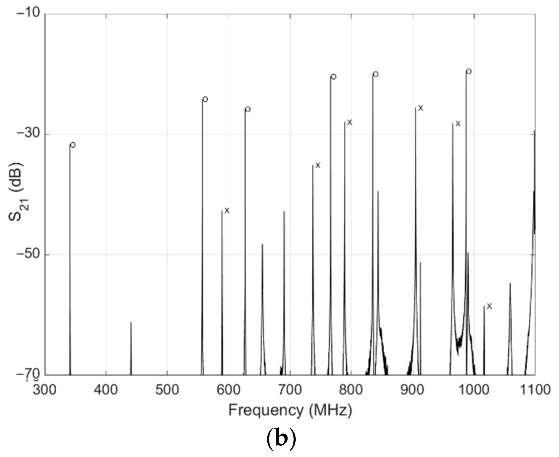
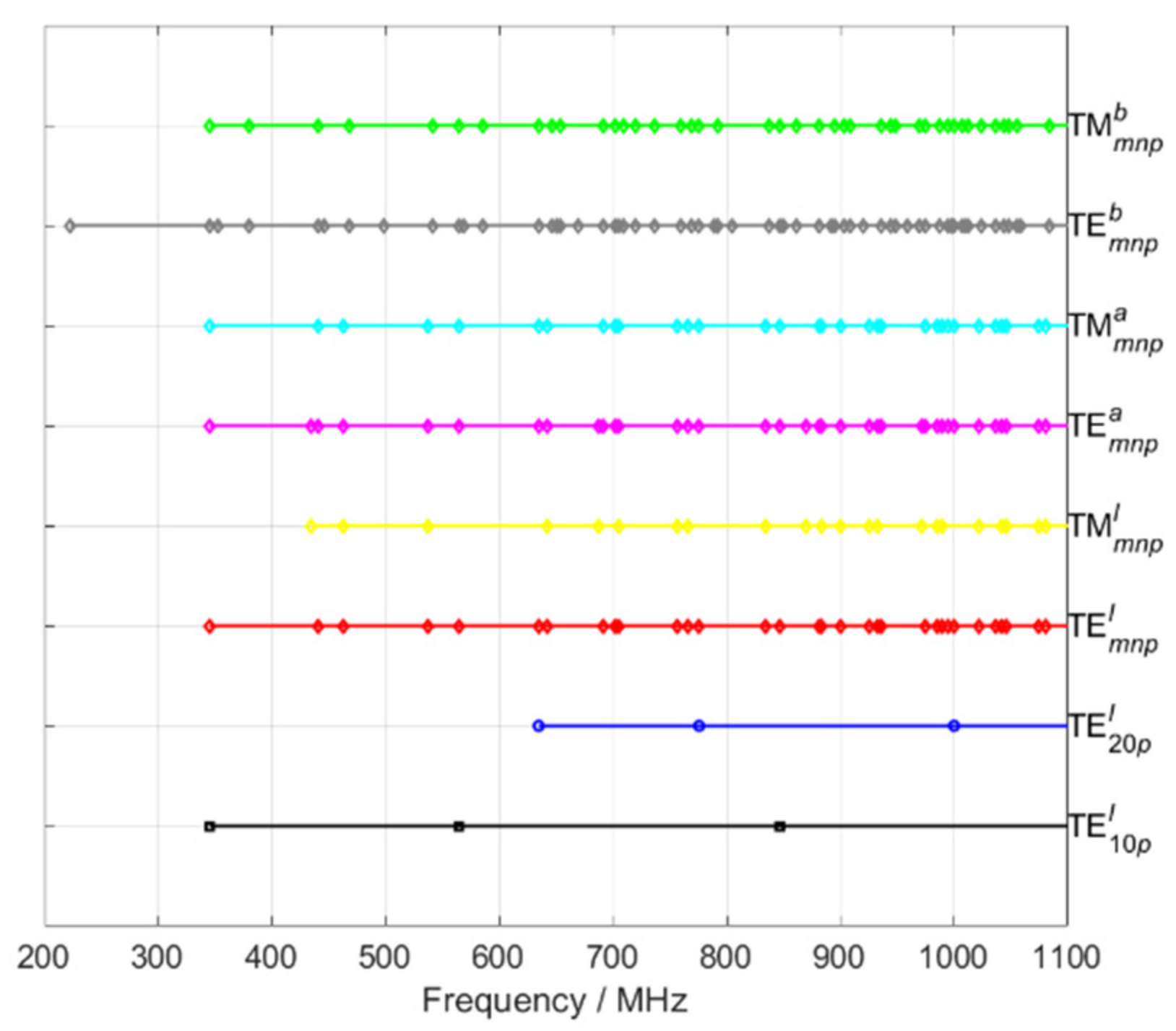
The permittivity ε_r and loss tangent tanδ calculated as (12) and (15) are based on the perturbation method with some approximation. To obtain exact results, the rigorous field analysis is needed.

The total fields in the first half part of the cavity for the TE^l_m0p mode loaded with a thin dielectric slab with the permittivity ε_r and the thickness t into the middle slot can be written as

$$\begin{array}{l}{E}_x=0\\ E_y=\frac{\omega {\mu }_{0}m\pi }{k_c^{2}a}\sin \frac{m\pi x}{a}\left\{\begin{array}{cc}A\sin {\beta }_{0}z,& 0<z<\left(l-t\right)/2\\ B\cos {\beta }_1\left(l/2-z\right),& \left(l-t\right)/2<z<l/2\end{array}\right.\\ E_z=0\\ H_x=-\frac{m\pi }{k_c^{2}a}\sin \frac{m\pi x}{a}\left\{\begin{array}{cc}A{\beta }_0\cos {\beta }_{0}z,& 0<z<\left(l-t\right)/2\\ B{\beta }_1\sin {\beta }_1\left(l/2-z\right),& \left(l-t\right)/2<z<l/2\end{array}\right.\\ H_y=0\\ H_z=\mathrm{j}\cos \frac{m\pi x}{a}\left\{\begin{array}{cc}A\sin {\beta }_{0}z,& 0<z<\left(l-t\right)/2\\ B\cos {\beta }_1\left(l/2-z\right),& \left(l-t\right)/2<z<l/2\end{array}\right.\end{array}$$

(16)

where β₀ and β₁ are the propagation constants in air and dielectric, respectively.

With the boundary condition that E_y and H_x should be continuous across the air-dielectric interface, we have

$${\beta }_1\tan {\beta }_0\frac{l-t}{2}={\beta }_0\mathrm{ctg}{\beta }_1\frac{t}{2}$$

(17)

The characteristic Equation (17) is a transcendental equation which can be solved numerically, such as the Newton method or the steepest descent method.

Using (14), we have the total stored energy of the loaded cavity, the conductor loss, and the dielectric loss as

$$\begin{array}{cc}W& ={\epsilon }_0{\displaystyle {\int }_0^a{\displaystyle {\int }_0^b{\displaystyle {\int }_0^{\left(l-t\right)/2}{\left|E_y\right|}^2\mathrm{d}x\mathrm{d}y\mathrm{d}z+{\epsilon }_0{\epsilon }_r{\displaystyle {\int }_0^a{\displaystyle {\int }_0^b{\displaystyle {\int }_{\left(l-t\right)/2}^{l/2}{\left|E_y\right|}^2\mathrm{d}x\mathrm{d}y\mathrm{d}z}}}}}}\\ & =\frac{{\epsilon }_0{\omega }^2{\mu }_0{}^2{m}^2{\pi }^{2}b}{2k_c^4{a}^{}}\left[\frac{A^2}{2}\left(\frac{l-t}{2}-\frac{\sin {\beta }_0\left(l-t\right)}{2{\beta }_0}\right)+\frac{{\epsilon }_r{B}^2}{2}\left(\frac{t}{2}+\frac{\sin {\beta }_{1}t}{2{\beta }_1}\right)\right]\hfill \end{array},$$

(18)

$$\begin{array}{cc}\hfill & P_c=R_s{\int }_0^a{\int }_0^b{H}^2{|}_{z=0}\mathrm{d}x\mathrm{d}y+R_s{\int }_0^a{\int }_0^l{H}^2{|}_{y=0}\mathrm{d}x\mathrm{d}z+R_s{\int }_0^l{\int }_0^b{H}^2{|}_{x=0}\mathrm{d}z\mathrm{d}y\hfill \\ \hfill & =\sqrt{\frac{\omega {\mu }_0}{2\sigma }}\left\{\begin{array}{cc}\hfill & \frac{A^2{{\beta }_0}^2{m}^2{\pi }^{2}b}{2k_c^{4}a}\hfill \\ \hfill & +\frac{m^2{\pi }^2}{k_c^{4}a}\left[\frac{A^2{{\beta }_0}^2}{2}\left(\frac{l-t}{2}+\frac{sin{\beta }_0\left(l-t\right)}{2{\beta }_0}\right)+\frac{B^2{{\beta }_1}^2}{2}\left(\frac{t}{2}-\frac{sin{\beta }_{1}t}{2{\beta }_1}\right)\right]\hfill \\ \hfill & +a\left[\frac{A^2}{2}\left(\frac{l-t}{2}-\frac{sin{\beta }_0\left(l-t\right)}{2{\beta }_0}\right)+\frac{B^2}{2}\left(\frac{t}{2}+\frac{sin{\beta }_{1}t}{2{\beta }_1}\right)\right]\hfill \\ \hfill & 2b\left[\frac{A^2}{2}\left(\frac{l-t}{2}-\frac{sin{\beta }_0\left(l-t\right)}{2{\beta }_0}\right)+\frac{B^2}{2}\left(\frac{t}{2}+\frac{sin{\beta }_{1}t}{2{\beta }_1}\right)\right]\hfill \end{array}\right\}\hfill \end{array},$$

(19)

and

$$\begin{array}{c}{P}_d=\omega \epsilon \tan \delta {\displaystyle {\int }_0^a{\displaystyle {\int }_0^b{\displaystyle {\int }_{\left(l-t\right)/2}^{l/2}{E}_y^2\mathrm{d}x\mathrm{d}y\mathrm{d}z}}}\\ ={\epsilon }_0{\epsilon }_r\tan \delta \frac{{\omega }^3{\mu }_0{}^2{m}^2{\pi }^{2}b{B}^2}{8k_c^{4}a}\left(t+\frac{\sin {\beta }_{1}t}{{\beta }_1}\right)\end{array}$$

(20)

respectively.

From the definition of quality factor, we have

$$\frac{1}{Q_L}=\frac{1}{Q_c}+\frac{1}{Q_d}=\frac{P_c+P_d}{\omega W}$$

(21)

If the resonant frequency of the loaded cavity f, the permittivity of the material under test ε_r, and the conductivity of the metallic walls σ are known, the total stored energy W and the conductor loss P_c can be calculated with (18) and (19), respectively. Consequentially, the dielectric loss P_d can be calculated from (21), and then the loss tangent of the material under test tanδ from (20), as long as the loaded quality factor Q_L is obtained.

3. Simulation

The measurement setup is simulated with the help of an independent software Ansoft HFSS which is basically a numerical 3-D electromagnetic field simulator based on the finite element method. The purpose of the simulation is to confirm the accuracy of the proposed method for calculating uniaxial isotropic permittivity from transmission coefficient data.

The simulated transmission coefficient in the band of 300 MHz to 1100 MHz is shown in Figure 6. The modes used for the permittivity measurement being marked with ‘o’ are TE^l₁₀₁, TE^l₁₀₃, TE^l₂₀₁, TE^l₂₀₃, TE^l₁₀₅, and TE^l₂₀₅, in the order of the frequency increasement. The interference modes marked with ‘x’ are TM^b₁₁₁, TM^b₁₃₁, TM^b₂₁₁, TM^b₂₃₁, TM^b₁₅₁, and TM^b₁₁₂, in the order of the frequency increasement. In the simulation model, the cavity walls are aluminum alloy with conductivity of 3.8 × 10⁷ S/m.

The electric field of all six measurement modes in the area of the middle slot of the rectangular cavity is in y-axis. The relative permittivity tensor of uniaxially anisotropic materials set in the simulation model is

$${\overline{\overline{\epsilon }}}_r=\left[\begin{array}{ccc}{\epsilon }_{r\parallel }& 0& 0\\ 0& {\epsilon }_{r\perp }& 0\\ 0& 0& {\epsilon }_{r\perp }\end{array}\right]=\left(1-\mathrm{j}0.0002\right)\left[\begin{array}{ccc}4& 0& 0\\ 0& 2.1& 0\\ 0& 0& 2.1\end{array}\right]$$

(22)

The cavity only responds to the permittivity tensor component that is parallel with y-axis, namely, electric field. In the simulation, the axis of the material under test is firstly set in y-axis. The cavity senses a material with permittivity of 4. Then, the axis of the material under test is set in x-axis. The cavity senses a material with permittivity of 2.1. The thickness of the material under test is 10 mm.

The calculated results are shown in

Table 1. Calculated permittivity and loss tangent from simulation results.

		TEl101	TEl103	TEl201	TEl203	TEl105	TEl205
Empty freq (MHz)		345	564	634	775	846	999
Empty Q-factor		32,579	48,835	42,299	51,322	61,549	62,201
∥	Loaded freq (MHz)	334	547	611	753	821	971
	Loaded Q-factor	19,768	27,040	20,492	28,806	31,549	31,836
	εr	3.98	3.96	3.99	3.98	3.96	3.96
	tanδ	0.00020	0.00020	0.00020	0.00020	0.00019	0.00021
⊥	Loaded freq (MHz)	341	558	627	767	837	988
	Loaded Q-factor	24,184	33,744	29,417	35,045	40,218	42,320
	εr	2.09	2.09	2.10	2.09	2.09	2.09
	tanδ	0.00020	0.00020	0.00020	0.00020	0.00018	0.00019

. The permittivity ε_r and the loss tangent tanδ are calculated from the transmission coefficient data by two methods. They are the perturbation method and the rigorous iterative method provided in Section 2.2 and 2.3, respectively. The results of the perturbation method are used as initial values for the rigorous iterative method. In this paper, only the results of the rigorous iterative method are given in Table 1. The modeled complex permittivity for the parallel (∥) and perpendicular (⊥) components are set as (22). The modeled and extracted results by the rigorous iterative method are in great agreement.

4. Measurement

After validating the proposed algorithm against the simulated data, an appropriate experimental setup is established in order to facilitate the measurement of transmission coefficient data. The Anritsu MS46322B Vector Network Analyzer (VNA) is used to obtain the transmission coefficient. The sweep parameters of the VNA are set as 201 points and 30 kHz IFBW. Due to the difficulty in producing samples with known anisotropic dielectric properties, the validity of the proposed method is demonstrated by measuring the permittivity of polytetrafluoroethylene (PTFE).

The fabricated multi-mode split rectangular cavity is shown in Figure 7. The cavity is made of aluminum alloy. Several aluminum alloy plates are screwed together to form the cavity. The inner side of the cavity is coated with silver. The inner conductor of the connector extrudes 8 mm into the cavity to act as the feeding pin. The coaxial line used to connect the VNA ports to the feeding pins does not have to be phase-stable cable. No amplifier is used. The transmission coefficient data of the empty and loaded cavity are measured, and they are shown in Figure 8. The loading material under test is a sheet of PTFE with a thickness of 10 mm. It can be seen that the measured result in Figure 8a is similar to the simulated result in Figure 6.

The permittivity ε_r and the loss tangent tanδ are calculated from the measured data in the same way as from the simulated data. The results given in

Table 2. Calculated results from measurement data.

	TEl101	TEl103	TEl201	TEl203	TEl105	TEl205
Empty freq (MHz)	341	557	627	766	835	987
Empty Q-factor	34,628	53,473	45,149	54,996	62,859	63,700
Loaded freq (MHz)	341	557	627	766	835	987
Loaded Q-factor	26,863	37,586	31,113	38,219	41,536	42,483
εr	2.04	2.04	2.06	2.05	2.04	2.05
tanδ	0.00019	0.00019	0.00021	0.00019	0.00020	0.00019

correspond to these known properties of PTFE (ε_r = 2.06, tanδ = 2 × 10⁻⁴) [44]. The variations of the measured permittivity ε_r and the loss tangent tanδ are less than 1% and 1 × 10⁻⁵, respectively, among all six modes.

5. Conclusions

In this paper, a multi-mode split cavity is designed and fabricated. A large number of interference modes are suppressed by the introduction of extra slots and deliberate choice of feed positions. Complex permittivity measurements of low-loss anisotropic materials are realized by using this cavity at hundreds of megahertz for the first time. The perturbation method and the rigorous iterative method are provided to calculate the permittivity from transmission coefficient. The validity and high precision of the method are demonstrated by simulation and measurement data. The cavity performance verifies its application in the complex permittivity measurement of low-loss cellular materials at hundreds of megahertz.

References

1. Hasar, U.C.; Bute, M. Electromagnetic characterization of thin dielectric materials from amplitude-only measurements. IEEE Sens. J. 2017, 17, 5093–5103. [Google Scholar] [CrossRef]
2. Costa, F.; Borgese, M.; Degiorgi, M.; Monorchio, A. Electromagnetic characterization of materials by using transmission/reflection (T/R) devices. Electronics 2017, 6, 95. [Google Scholar] [CrossRef] [Green Version]
3. Krupka, J. Frequency domain complex permittivity measurements at microwave frequencies. Meas. Sci. Technol. 2006, 17, 55–70. [Google Scholar] [CrossRef]
4. Nicolson, A.; Ross, G. Measurement of the intrinsic properties of materials by time-dome techniques. IEEE Trans. Instrum. Meas. 1970, 19, 791–795. [Google Scholar] [CrossRef] [Green Version]
5. Gorriti, A.; Slob, E. A new tool for accurate S-parameters measurements and permittivity reconstruction. IEEE Trans. Geosci. Remote Sens. 2005, 43, 1722–1735. [Google Scholar] [CrossRef]
6. Weir, W. Automatic measurement of complex dielectric constant and permeability at microwave frequency. Proc. IEEE 1974, 62, 33–36. [Google Scholar] [CrossRef]
7. Akhtar, M.; Feher, L.; Thumm, M. A waveguide-based two-step approach for measuring complex permittivity tensor of uniaxial composite materials. IEEE Trans. Microw. Theory Tech. 2006, 54, 2011–2022. [Google Scholar] [CrossRef]
8. Wu, C.; Liu, Y.; Lu, S.; Gruszczynski, S.; Yashchyshyn, Y. Convenient waveguide technique for determining permittivity and permeability of materials. IEEE Trans. Microw. Theory Tech. 2020, 68, 4905–4912. [Google Scholar] [CrossRef]
9. Shahpari, M. Determination of complex conductivity of thin strips with a transmission method. Electronics 2019, 8, 21. [Google Scholar] [CrossRef] [Green Version]
10. Catala-Civera, J.; Canos, A.; Penarand-Foix, F.; Davos, E. Accurate determination of the complex permittivity of materials with transmission reflection measurements in partially filler rectangular waveguides. IEEE Trans. Microw. Theory Tech. 2003, 51, 16–24. [Google Scholar] [CrossRef]
11. Hasar, U. Accurate complex permittivity inversion from measurements of a sample partially filling a waveguide aperture. IEEE Trans. Microw. Theory Tech. 2010, 58, 451–457. [Google Scholar] [CrossRef]
12. Bao, X.; Wang, L.; Wang, Z.; Zhang, J.; Zhang, M.; Crupi, G.; Zhang, A. Simple, fast, and accurate broadband complex permittivity characterization algorithm: Methodology and experimental validation from 140 GHz up to 220 GHz. Electronics 2022, 11, 366. [Google Scholar] [CrossRef]
13. Ghodgaonkar, D.K.; Varadan, V.V.; Varadan, V.K. Free-space measurement of complex permittivity and complex permeability of magnetic materials at microwave frequencies. IEEE Trans. Instrum. Meas. 1990, 39, 387–394. [Google Scholar] [CrossRef]
14. Hasar, U.C. Non-destructive testing of hardened cement specimens at microwave frequencies using a simple free-space method. NDTE Int. 2009, 42, 550–557. [Google Scholar] [CrossRef]
15. Hegler, S.; Seiler, P.; Dinkelaker, M.; Schladitz, F.; Plettemeier, D. Electrical material properties of carbon reinforced concrete. Electronics 2020, 9, 857. [Google Scholar] [CrossRef]
16. Yang, X.; Liu, X.; Yu, S.; Gan, L.; Zhou, J.; Zeng, Y. Permittivity of undoped silicon in the millimeter wave range. Electronics 2019, 8, 886. [Google Scholar] [CrossRef] [Green Version]
17. Gonçalves, F.J.F.; Pinto, A.G.M.; Mesquita, R.C.; Silva, E.J.; Brancaccio, A. Free-space materials characterization by reflection and transmission measurement using frequency-by-frequency and multi-frequency algorithms. Electronics 2018, 7, 260. [Google Scholar] [CrossRef] [Green Version]
18. Eyraud, C.; Geffrin, J.M.; Litman, A.; Tortel, H. Complex permittivity determination from far-field scattering patterns. IEEE Antennas Wirel. Propag. Lett. 2015, 14, 309–312. [Google Scholar] [CrossRef]
19. Abbato, R. Dielectric constant measurements using RCS data. Proc. IEEE 1965, 53, 1095–1097. [Google Scholar] [CrossRef]
20. Horner, F.; Taylor, T.A.; Dunsmuir, R.; Lamb, J.; Jackson, W. Resonance methods of dielectric measurement at centimetre wavelength. J. Inst. Electr. Eng.-Part III Radio Commun. Eng. 1946, 93, 53–68. [Google Scholar]
21. Krupka, J.; Milewski, A. Accurate method of the measurement of complex permittivity of semiconductors in H01n cylindrical cavity. Electron. Technol. 1978, 11, 11–31. [Google Scholar]
22. Li, S.; Akyel, C.; Bosisio, R.G. Precise calculations and measurement on the complex dielectric constant of lossy materials using TM010 perturbation techniques. IEEE Trans. Microw. Theory Tech. 1981, 29, 1041–1048. [Google Scholar]
23. Risman, P.O.; Ohlsson, T. Theory for and experiments with a TM020 applicator. J. Microw. Power 1975, 10, 271–280. [Google Scholar] [CrossRef]
24. Ma, J.; Wu, Z.; Xia, Q.; Wang, S.; Tang, J.; Wang, K.; Guo, L.; Jiang, H.; Zeng, B.; Gong, Y. Complex permittivity measurement of high-loss biological material with improved cavity perturbation method in the range of 26.5–40 GHz. Electronics 2020, 9, 1200. [Google Scholar] [CrossRef]
25. Jha, A.K.; Akhtar, M.J. A generalized rectangular cavity approach for determination of complex permittivity of materials. IEEE Trans. Instrum. Meas. 2014, 63, 2632–2641. [Google Scholar] [CrossRef]
26. Jones, R.G. Precise dielectric measurements at 35 GHz using a microwave open-resonator. Proc. Inst. Electr. Eng. 1976, 123, 285–290. [Google Scholar] [CrossRef]
27. Lynch, A.C.; Clarke, R.N. Open resonators: Improvement of confidence in measurement of loss. IEEE Proc. 1992, 139, 221–225. [Google Scholar] [CrossRef]
28. Hakki, B.W.; Coleman, P.D. A dielectric resonator method of measuring inductive capacities in the millimeter range. IEEE Trans. Microw. Theory Tech. 1960, 8, 402–410. [Google Scholar] [CrossRef]
29. Kobayashi, Y.; Katoh, M. Microwave measurement of dielectric properties of low-loss materials by the dielectric rod resonator method. IEEE Trans. Microw. Theory Tech. 1985, 33, 586–592. [Google Scholar] [CrossRef]
30. Krupka, J.; Derzakowski, K.; Riddle, B.; Baker-Jarvis, J. A dielectric resonator for measurements of complex permittivity of low loss dielectric materials as a function of temperature. Meas. Sci. Technol. 1998, 9, 1751–1756. [Google Scholar] [CrossRef]
31. Krupka, J.; Huang, W.T.; Tung, M.J. Complex permittivity measurements of low loss microwave ceramics employing higher order quasi TE0np modes excited in a cylindrical dielectric sample. Meas. Sci. Technol. 2005, 16, 1014–1020. [Google Scholar] [CrossRef]
32. Krupka, J.; Derzakowski, K.; Abramowicz, A.; Tobar, M.E.; Geyer, R.G. Whispering gallery modes for complex permittivity measurements of ultra-low loss dielectric materials. IEEE Trans. Microw. Theory Tech. 1999, 47, 752–759. [Google Scholar] [CrossRef]
33. Krupka, J.; Derzakowski, K.; Tobar, M.E.; Hartnett, J.; Geyer, R.G. Complex permittivity of some ultralow loss dielectric crystals at cryogenic temperatures. Meas. Sci. Technol. 1999, 10, 387–392. [Google Scholar] [CrossRef]
34. Roelvink, J.; Trabelsi, S.; Nelson, S.O. Measuring the complex permittivity tensor of uniaxial biological materials with coplanar waveguide transmission line. IEEE Microw. Wirel. Compon. Lett. 2014, 24, 811–813. [Google Scholar] [CrossRef]
35. Hashimoto, O.; Shimizu, Y. Reflecting characteristics of anisotropic rubber sheets and measurement of complex permittivity tensor. IEEE Trans. Microw. Theory Tech. 1986, 34, 1202–1207. [Google Scholar] [CrossRef]
36. Damaskos, N.J.; Mack, R.B.; Maffett, A.L.; Parmon, W.; Uslenghi, P.L.E. The inverse problem for biaxial materials. IEEE Trans. Microw. Theory Tech. 1984, 32, 400–405. [Google Scholar] [CrossRef]
37. Belhadj-Tahar, N.E.; Fourrier-Lamer, A. Broad-band simultaneous measurement of the complex permittivity tensor for uniaxial materials using a coaxial discontinuity. IEEE Trans. Microw. Theory Tech. 1991, 39, 1718–1724. [Google Scholar] [CrossRef]
38. Kobayashi, Y.; Tanaka, S. Resonant modes of a dielectric rod resonator short-circuited at both ends by parallel conducting plates. IEEE Trans. Microw. Theory Tech. 1980, 28, 1077–1085. [Google Scholar] [CrossRef]
39. Geyer, R.G.; Krupka, J. Microwave dielectric properties of anisotropic materials at cryogenic temperatures. IEEE Trans. Instrum. Meas. 1995, 44, 329–331. [Google Scholar] [CrossRef]
40. Krupka, J.; Geyer, R.G.; Kuhn, M.; Hinken, J. Dielectric properties of single crystal Al2O3, LaAlO3, NdGaO3, SrTiO3, and MgO at cryogenic temperatures and microwave frequencies. IEEE Trans. Microw, Theory Tech. 1994, 42, 1886–1890. [Google Scholar] [CrossRef]
41. Chen, L.; Ong, C.K.; Tan, B.T.G. Cavity perturbation technique for the measurement of permittivity tensor of uniaxially anisotropic dielectrics. IEEE Trans. Instrum. Meas. 1999, 48, 1023–1030. [Google Scholar] [CrossRef]
42. Mumcu, G.; Sertel, K.; Volakis, J.L. A measurement process to characterize natural and engineered low-loss uniaxial dielectric materials at microwave frequencies. IEEE Trans. Microw. Theory Tech. 2008, 56, 217–223. [Google Scholar] [CrossRef]
43. Kopyt, P.; Salski, B.; Krupka, J. Measurements of complex anisotropic permittivity of laminates with TM0n0 cavity. IEEE Trans. Microw. Theory Tech. 2022, 70, 432–443. [Google Scholar] [CrossRef]
44. Baker-Jarvis, J.; Riddle, B.; Janezic, M.D. Dielectric and Magnetic Properties of Printed Wiring Boards and Other Substrate Materials; NIST: Gaithersburg, MD, USA, 1999; p. 1512. [Google Scholar]
Figure 1. The geometry of a rectangular cavity.
Electronics 11 01769 g001
Figure 2. All resonant frequencies of the rectangular cavity.
Electronics 11 01769 g002
Figure 3. The final rectangular cavity with many interference modes suppressed.
Electronics 11 01769 g003
Figure 4. The measurement and interference resonant frequencies of the final rectangular cavity.
Electronics 11 01769 g004
Figure 5. Top view of the cavity loaded with the material under test.
Electronics 11 01769 g005
Figure 6. Simulated transmission coefficient of the empty cavity. Measurement modes are marked with ‘o’, while interference modes ‘x’.
Electronics 11 01769 g006
Figure 7. Photograph of the fabricated cavity with the sample under test.
Electronics 11 01769 g007
Figure 8. Simulated transmission coefficient of the cavity: (a) empty and (b) loaded. Measurement modes are marked with ‘o’, while interference modes are marked with ‘x’.
Electronics 11 01769 g008aElectronics 11 01769 g008b