Spectrum Anomaly Detection Based on Spatio-Temporal Network Prediction

Abstract

With the miniaturization of communication devices, the number of distributed electromagnetic devices is increasing. In order to achieve effective management of the electromagnetic spectrum, prediction and anomaly detection of the spectrum has become increasingly critical. This paper proposes an algorithmic framework for detecting spectrum anomalies using deep learning techniques. More specifically, the framework includes spectrum prediction and anomaly detection. We use the sliding window method to divide the time series, construct multi-timescale historical data, and train the model with normal data to have high accuracy spectrum prediction capability. We analyze and determine the discriminant function to distinguish the spectral anomalies by calculating the differences between the predicted and real data. The experimental results show that the proposed method outperforms existing baseline algorithms based on real-world spectrum measurement data and simulated anomaly data.

1. Introduction

In recent years, communication technology has developed rapidly, and the process of miniaturization, portability, and intelligence of communication equipment has intensified. The electromagnetic environment is becoming more and more complex, and radio spectrum resources are becoming more and more precious. In order to improve spectrum utilization and alleviate spectrum scarcity, spectrum sharing and dynamic spectrum access have been successively introduced [1]. However, the work of dynamic spectrum access is exposed to the risk of various attacks. Therefore, spectrum anomaly detection techniques have been widely focused on and have gradually become a hot topic in cognitive radio. Spectrum anomaly detection is an essential component in cognitive radio and spectrum monitoring, enabling the detection of anomalies such as malicious interference, user conflicts, and illegal occupancy to improve communication quality [2]. At the same time, spectrum anomaly detection and research are essential for radio equipment management and electromagnetic environment posture assessment [3].

Anomaly detection algorithms are generally divided into two types: the first based on appropriate feature extraction for event representation, and the second is to establish a model that can evaluate whether an event is an anomaly [4]. Traditional electromagnetic spectrum anomaly detection algorithms are based on feature extraction. Kullback–Leibler Divergence [5], Brier’s-Score [6], Compressed-Sensing [7], Random-Forest [8], Hidden-Markov [9], Fractional Fourier [10], and Machine Learning [11] have also been used for anomaly detection and achieved certain results. With the continuous development of the artificial intelligence industry, deep learning has demonstrated its powerful data analysis ability and scholars have made some achievements in anomaly detection using deep learning. The data is encoded and downscaled by deep networks to achieve feature extraction, combined with clustering methods to achieve anomaly detection [12,13]. This feature-extraction-based approach has some anomaly detection capability, but its anomaly detection results depend heavily on the expressiveness of the features and the results of the clustering algorithm. In addition, biased data in the training data can cause the clustering algorithm to be biased and affect the anomaly detection results.

Without using the basic features of the data in the study of this paper, the focus is on building a network model that enables anomaly detection. Existing algorithms discriminate anomalies by reconstruction error and prediction error, and some results have been achieved. SAIFE is a spectrum anomaly detection algorithm based on an adversarial autoencoder (AAE) [14]. The system can realize anomaly detection by discriminating reconstruction errors of received spectrum data. LSTM networks can detect a variety of abnormal states in the LTE signal spectrum by predicting spectral data and can detect anomalies across the frequency band by transfer learning [15]. In order to solve the abnormal spectrum status in satellite communication, LSTM networks can realize the detection of multi-variable abnormal states and subtle abnormal states on the basis of spectrum prediction [16]. The encoder is combined with the GAN network to form a new anomaly detection network. Compared with the conventional model, the encoder module is added to the algorithm to realize anomaly detection based on reconstruction errors; however, the system network complexity is high [17]. In the case of small samples, ACGAN is able to expand the training samples to achieve anomaly detection of spectral data [18]. In general, the anomaly detection algorithm based on reconstruction still achieves data feature selection, extraction, and dimensionality reduction through the deep network but is still affected by deviated data and has poor sensitivity to low power spectrum anomalies. In contrast, the spectral anomaly detection algorithm based on the prediction method can not only make full use of the time sequence characteristics of data but also realize the detection of low-power anomalies with high prediction accuracy [19,20,21]. However, existing anomaly detection algorithms, whether based on reconstruction or prediction methods, do not take full advantage of historical data. Existing algorithms use historical spectral data to produce the dataset required for deep learning and have taken the data in a sliding window to train a deep model. However, this approach fails to take into account the spatial and temporal correlation of spectrum data. In fact, most of the frequency-using devices are affected by time variation, and the data intensity of some frequency bands has a periodical variation with time in terms of days. Therefore, this paper processes the historical data from different time scales into the depth model, which has obtained higher accuracy of spectrum prediction and thus improved the anomaly detection performance of the model.

Scholars have obtained some research results regarding ways of inputting the obtained historical data at different scales into the network and obtain and fuse the features. Existing algorithms [22,23] input historical data processed at three-time scales into different branches of the network in parallel and obtain prediction results through feature fusion. However, inputting historical data from different time scales into the depth model in a parallel mode may result in redundancy of data leading to degradation of prediction performance. The parallel input mode requires a lot of repetition of the feature extraction modules in the network, and the number of algorithm parameters increases significantly. In fact, in order to input historical data on a time scale of days and hours into the deep network, it is necessary to average them over time. After processing, the short-term change characteristics of the data become blurred, and the trend characteristics become more obvious. Since the correlation of spectrum data is strong in a short period, the prediction of spectrum data in the next moment mainly relies on the spectrum data in a short time period, and the historical data processed on a large scale should assist the short-time-period spectrum data in improving the prediction performance.

In order to make full use of the multi-timescale historical data and achieve efficient anomaly detection of spectrum data, this paper proposes a framework for spectrum anomaly detection based on spatio-temporal network prediction. Firstly, we analyze the spectrum data, set the historical data in the time scale of days and hours, and use the sliding window method to construct the data set; then, we build a deep network capable of fusing multiple moderate temporal features, which uses the LSTM module to mine the temporal features of the data in a multi-timescale and combine the short-time-period spectral features extracted by the convolutional network to realize the spectrum prediction. Finally, the identification function is analyzed and determined to compare the differences between the predicted and received data to achieve anomaly detection. Experiments are conducted on several frequency bands, and the experimental results show that the anomaly detection algorithm based on spatio-temporal network prediction proposed in this paper is superior to the existing algorithms.

The main contributions are as follows:

• We analyze the historical spectrum data to clarify the periodicity of most frequency bands and the length of the period. The data are processed on a time scale of days and hours, and the data set is generated using a sliding window approach.
• A spectrum prediction network that can make full use of multi time scale historical information is designed. The network contains depth feature extraction modules and a multi-timescale feature extraction module, which can effectively extract the features of spectrum data at different time scales.
• Comparative analysis of the discriminatory function and anomaly detection experiments in multiple frequency bands verify the rationality of the anomaly detection algorithm framework in this paper.

The rest of this paper is organized as follows. In Section 2, the problem of anomaly detection based on spectrum prediction is clearly stated. In Section 3, a spectrum prediction model capable of fusing multi-timescale data is proposed, and each feature extraction module is explained in detail. In Section 4, experimental results are given, and the performance is evaluated. Conclusions and suggestions for future work are presented in Section 5.

2. Problem Description of Anomaly Detection Based on Spectrum Prediction

The main task of spectrum anomaly detection is to detect the received spectrum data and clarify whether it contains anomalous signals or anomalous interference. To describe the anomaly detection problem in detail, we first model the received signal as shown in Equation (1).

$$\begin{array}{c}\left\{\begin{array}{c}{H}_0:r\left(n\right)=s\left(n\right)+w\left(n\right),n=1,\cdots ,N\hfill \\ H_1:r\left(n\right)=j\left(n\right)+s\left(n\right)+w\left(n\right),n=1,\cdots ,N\hfill \end{array}\right.\hfill \end{array}$$

(1)

where, $H_0$ and $H_1$ are conventional and abnormal data respectively, $r\left(n\right)$ is received signal, $s\left(n\right)$ is normal user data, $j\left(n\right)$ is abnormal interference signal, and $w\left(n\right)$ is noise signal, N is the number of received signals.

The variation in the time domain is an important feature in the use of spectrum, so we adopt STFT to represent the time-frequency of the received signal, as shown in Equation (2):

$$y(n,m)=\sum _{k=-\infty }^{\infty }r\left(k\right)g^{*}\left(k/\phantom{kF}F-n/\phantom{nF}F\right)e^{-j2\pi \left(mF\right)k},$$

(2)

where $g\left(n\right)$ represents the window function of a particular type and length, * denotes complex conjugate, F is the sampling rate, and m represents the cycle frequency depending on F. Unlike the traditional algorithms, which require complex statistical models and high computational complexity, the anomaly detection model based on deep learning can intelligently learn the data distribution $p\left(X_s\right)$ from the source data set $X_s$, and identify the anomaly when the test data deviates from the data distribution.

We use spectrum prediction to implement anomaly detection so that the problem can be further described. It is assumed that the spectrum data of the received signal is the measured value of F frequency points in T time slots, and the time-frequency domain sequence can be expressed in the form of a matrix in the simplified symbol, ${\mathbf{X}}_T^N={\left({\mathbf{x}}^1,{\mathbf{x}}^2,{\mathbf{x}}^3\cdots {\mathbf{x}}^N\right)}^{\mathrm{T}}=\left({\mathbf{x}}_1,{\mathbf{x}}_2,{\mathbf{x}}_3\cdots {\mathbf{x}}_T\right)\in {\mathbb{R}}^{N\times T}$. Where, ${\mathbf{x}}^i$ represents the collected data of each frequency point and is the row in the matrix. ${\mathbf{x}}_j$ represents the data at each time and is the column in the matrix, ${(•)}^{\mathrm{T}}$ means matrix transpose operation. Therefore, the time series data at the k frequency point can be represented as ${\mathbf{x}}^k={\left(x_1^k,x_2^k,\cdots ,x_T^k\right)}^{\mathrm{T}}\in {\mathbb{R}}^T$; similarly, the data at each frequency point at the t time can be represented as ${\mathbf{x}}_t={\left(x_t^1,x_t^2,\cdots ,x_t^N\right)}^{\mathrm{T}}\in {\mathbb{R}}^N$.

Conventional spectrum prediction is based on the spectrum data in a short period of time to predict the future multi-slot data. If the current moment is $T_1$ and the frequency point is k, the data ${\mathbf{X}}_s^k$ of the first s time slots is used to predict the data ${\widehat{\mathbf{X}}}_{\tau }^k$ of the future $\tau$ time slots, as shown in Formula (3) below.

$$\begin{array}{c}{\mathbf{X}}_s^k=\left(x_{T_1-s},x_{T_1-s+1},\cdots ,x_{T_1}\right)\in {\mathbb{R}}^{k\times s}\hfill \\ {\widehat{\mathbf{X}}}_{\tau }^k=F_x\left({\mathbf{X}}_s^k\right)\in {\mathbb{R}}^{k\times \tau }\hfill \end{array}$$

(3)

This paper proposes a prediction method based on a spatio-temporal network, which processes historical data at multi-timescale and combines spectral data in a short time period to further improve the prediction performance of the model. The historical data processed at different scales is defined as ${\mathbf{X}}_{scale}$, then the prediction model in this paper can be described as:

$$\widehat{\mathbf{X}}=F_{st}\left(\mathbf{X},{\mathbf{X}}_{scale}\right)\in {\mathbb{R}}^{k\times \tau }$$

(4)

If ${\mathbf{X}}^{*}$ is used to represent the real received data, $\widehat{\mathbf{X}}$ is the model-predicted data, the identification function is set as D, and the detection threshold is set as $\eta$, the anomaly detection process can be described as follows:

$$\left\{\begin{array}{c}{H}_1:D({\mathbf{X}}^{*},\widehat{\mathbf{X}})>\eta \hfill \\ H_0:D({\mathbf{X}}^{*},\widehat{\mathbf{X}})<\eta \hfill \end{array}\right.$$

(5)

3. Spectrum Anomaly Detection Framework

In this paper, we use deep learning to implement modelling of spectrum prediction. Most of the existing prediction-based anomaly detection algorithms use the temporal characteristics of the spectrum data to build a network using LSTM modules. They can enhance the prediction effect by appropriate structural transformations. Some algorithms treat the time-frequency data as images for processing and use convolutional networks to extract the depth features of the data. However, both of these structures have certain limitations. The LSTM module using temporal features cannot realize the parallel input of multidimensional data, which limits its feature extraction capability. The network performance is poor when the data contains many frequency points and a long time period. The model using convolutional networks can quickly extract depth features. However, when the spectrum data is highly volatile, it is difficult to obtain the change characteristics of the data, and the prediction performance has a significant decrease.

In addition, the existing algorithms do not make good use of the historical data and fail to adequately explore the change trends of the spectrum data on large time scales. Therefore, the spectrum historical data are analyzed to clarify the change trends of the spectrum data under different time scales. Then, referring to classical network structures such as U-Net [24], we propose a network structure combining convolutional and LSTM modules. The network consists of two deep feature extraction modules with convolutional kernels of different sizes and one multi-timescale feature extraction module. The network has a powerful feature extraction and fusion capability. Finally, the historical data are processed on the scale of days and hours, respectively. The prediction results are obtained by combining the spectrum data of a short period into the network. The anomaly detection is realized according to the difference between the predicted spectrum data and the received data.

3.1. Correlation Analysis of Spectrum Data

First, we briefly describe the data, simulation anomalies, and experimental conditions used in this paper. The spectrum data used in the experiments are divided into two main parts: the spectrum data from the publicly available network and the spectrum data collected by monitoring with a software radio device. In particular, the publicly available spectrum data were obtained from RWTH Aachen University. The researchers conducted rigorous and comprehensive spectrum measurements at two monitoring sites in Aachen, Germany, and one monitoring site in Ma, the Netherlands. The monitored frequency band ranges from 20 MHz to 6 GHz and includes four sub bands with a bandwidth of 1.5 GHz and a frequency point resolution of 200 kHz. In the measurements, the sweep interval is 1.8 s. The monitoring system can obtain power spectral density (PSD) values for 1000 frequency points every half hour, and the maximum period of continuous monitoring is about 14 days [25]. The data contains several commonly used frequency bands, such as GSM900 uplink (UL), GSM900 downlink (DL), TV, etc. A total of 6 data sets are generated based on the commonly used service bands. In addition, the data from multiple frequency bands will be collected and processed separately using Software Defined Radio (SDR) in Hefei, China, in February 2022. The SDR acquisition lasts for a few days, which is insufficient to support a multi-timescale prediction and anomaly detection framework. However, the data fluctuates and changes rapidly, so this dataset serves as an aid to verify the model performance in this paper. The available datasets are generated based on the active service bands in the two types of spectrum data, as shown in

Table 1. Spectrum Datasets Used in This Paper.

Spectrum Bands	Range (MHz)
Aachen Spectrum Dataset
GSM900 Uplink	877.6–902.4
GSM900 Downlink	935–959
GSM1800 Uplink	1710.2–1784.8
GSM1800 Downlink	1820.2–1875.4
TV Broadcast	614–698
ISM	2400.1–2483.3
Software Radio Dataset
GSM900 Uplink	889–909
GSM900 Downlink	934–954
TV Broadcast	546–566
FM	87–107

.

Spectral data can be regarded as a special kind of multidimensional time series. Unlike conventional multidimensional time series, the spectrum data contains more frequency points, and there is a strong correlation between the frequency points. In addition, the prediction-based spectrum anomaly detection is also different from the general time series anomaly detection. From the current state of research and problem description, it is clear that the input and output of spectral anomaly detection are matrices constructed from time-frequency data, which are fundamentally different in structure from time series anomaly detection. However, the spectrum data has similarities with regular time series and has some characteristics of time series. Data such as traffic flow, weather conditions, air quality, and room occupancy are influenced by human behaviour or environmental characteristics and are periodic on some time scale. Most of the frequency bands are also periodic due to the periodic nature of the behaviour of the frequency-using device or the primary user of the band. The Pearson correlation coefficient [26] is used as an indicator to analyze the correlation between the frequency band data from the time domain perspective, which is calculated as shown in Equation (6).

$${\rho }_{\mathbf{a},\mathbf{b}}=\frac{\mathrm{cov}\left(\mathbf{a},\mathbf{b}\right)}{{\sigma }_{\mathbf{a}}{\sigma }_{\mathbf{b}}}=\frac{E\left[\left(\mathbf{a}-{\mu }_{\mathbf{a}}\right)\left(\mathbf{b}-{\mu }_{\mathbf{b}}\right)\right]}{{\sigma }_{\mathbf{a}}{\sigma }_{\mathbf{b}}},$$

(6)

where, $\mathbf{a},\mathbf{b}$ represents two random variables, ${\mu }_{\mathbf{a}},{\mu }_{\mathbf{b}}$ represents sample mean, ${\sigma }_{\mathbf{a}},{\sigma }_{\mathbf{b}}$ represents sample standard deviation, $\mathrm{cov}(\ast )$ and $E\left[\ast \right]$ represent covariance and expectation operator.

Taking GSM1800 Uplink and GSM1800 Downlink as examples, the periodicity of spectrum data is analyzed by using detrending and Pearson correlation coefficient, and the results are shown in Figure 1 and Figure 2. In Figure 1b and Figure 2b, the sampled data at approximately 800-time points are used to represent the spectrum variation within a day. Continuous blocky areas appear in Figure 1b as well as in Figure 2b, which indicates the existence of correlation variations in the data in terms of days. It can also be found that both frequency bands contain a large number of points with correlations close to 1. Some of the points have a high correlation even though they have a long-time difference between them. This indicates that the spectrum history data show complex similarities and correlations on different time scales. In Figure 1c as well as in Figure 2c, the existence of a clear day-based cycle of the data can be found after detrending. The GSM 1800 Downlink band energy variation is relatively large, with a varied range of about 5 dBm. The signal strength shows a rising and then falling change during the day, which is also in line with the habits of cell phone users. The above analysis shows that some frequency bands have periodic changes and the historical data have a high correlation with the current spectrum data. In addition, the processing of historical data with different time scales can obtain the time pattern and magnitude pattern of spectrum data changes. The correlation and change pattern between the data can enable the depth model to obtain more information and improve the prediction results of the current spectrum state, thus improving the anomaly detection performance.

3.2. Algorithmic Framework

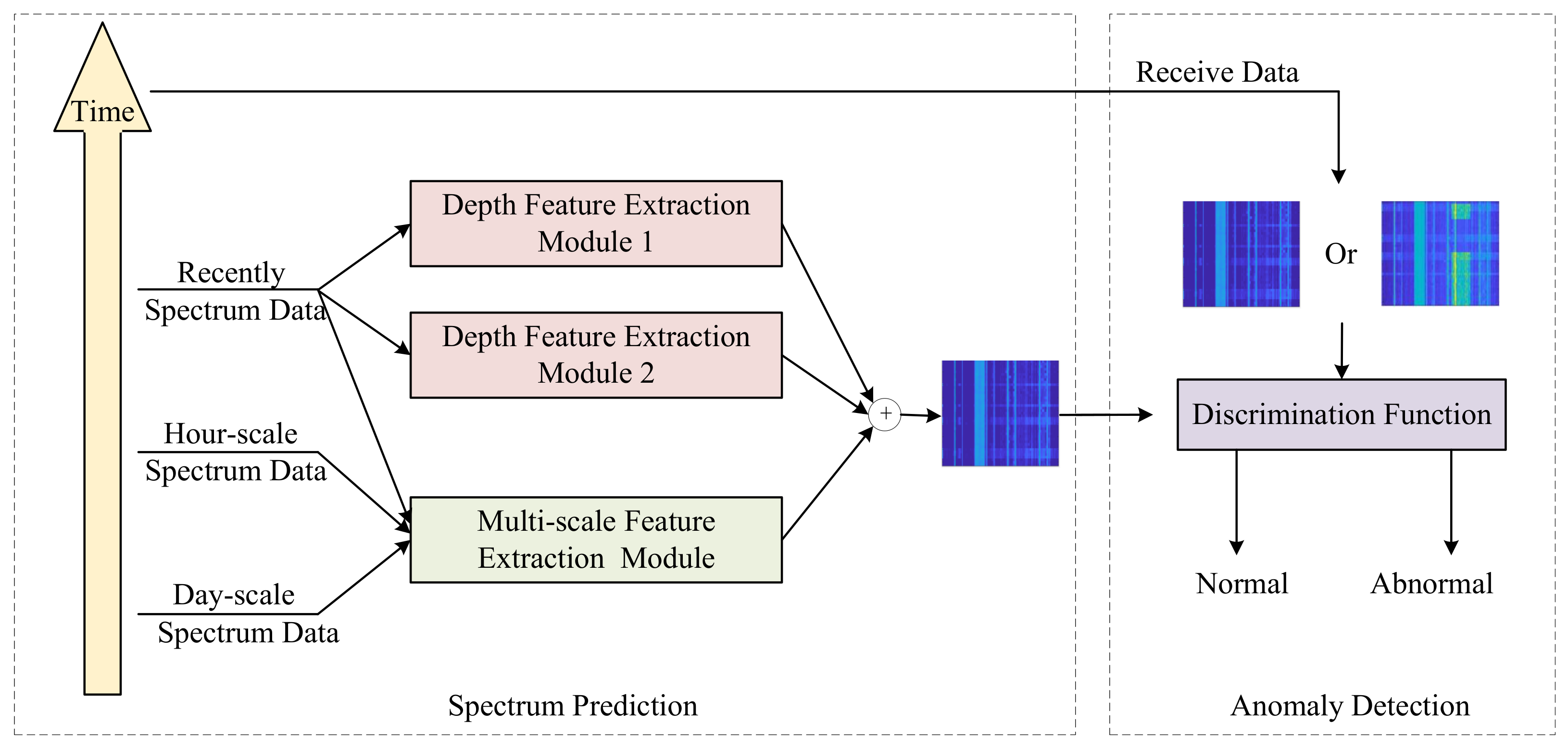
The overall framework of the proposed spectrum anomaly detection algorithm is shown in Figure 3, which can be divided into two parts: spectrum prediction and anomaly detection. First, we process the received historical data and extract the spectrum data in the short term, hourly scale, and day scale, respectively. Then, the spectrum data are fed into a spectrum prediction network containing different feature extraction modules to achieve spectrum prediction. Finally, the discrimination function calculates the difference between the predicted data and the actual received data, and when the difference exceeds a preset threshold, it is considered that there is an anomaly in the spectrum.

According to the previous description, the spectral history data of multiple time scales are represented in the form of a matrix. Then we use ${\mathbf{X}}_c$ to denote the spectrum data of a short period, ${\mathbf{X}}_{hours}$ to denote the spectrum data of every hour, and ${\mathbf{X}}_{days}$ to denote the spectrum data of a day. The data are processed in the form of sliding windows, and the continuous matrix is transformed into tensor form to generate the required dataset for training. The deep network for spectrum prediction in this paper consists of a depth feature extraction module and a multi-scale feature extraction module, which can extract different features of the data. The extracted features are selected and fused to achieve spectrum data prediction. If we use $M_{Deep}$ and $M_{Mutil}$ as the representation functions of the depth feature extraction module and the multi-scale feature extraction module, respectively, the process of feature fusion and spectrum prediction can be expressed as Equation (7). 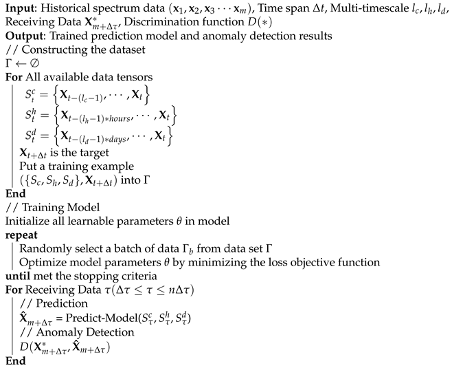Where $\mathbf{W}$ denotes the parameters that can be continuously optimized by learning, and ${\mathbf{X}}_{Mutil}$ denotes the combined data of different time scale data. The process of spectrum prediction is shown in Algorithm 1.

$$\begin{array}{c}\widehat{\mathbf{X}}={\mathbf{W}}_1{M}_{Deep1}\left({\mathbf{X}}_c\right)+{\mathbf{W}}_2{M}_{Deep2}\left({\mathbf{X}}_c\right)+{\mathbf{W}}_3{M}_{Mutil}\left({\mathbf{X}}_{Mutil}\right)\hfill \\ {\mathbf{X}}_{Mutil}=concatenate({\mathbf{X}}_c,{\mathbf{X}}_{hours},{\mathbf{X}}_{days})\hfill \end{array}$$

(7)

Algorithm 1 Spectrum anomaly detection algorithm using deep learning

3.3. Feature Extraction Module

3.3.1. Depth Feature Extraction Module

If the time-frequency data matrix is treated as an image, then the spectral data prediction problem can be transformed into an image prediction problem. Convolutional neural networks exhibit powerful image information processing capability and can better extract depth information from the time-frequency data. CNN is a class of feedforward neural networks that includes convolutional computation and has a deep structure with powerful representation learning capability. Through convolutional operations, CNN can realize the change of data dimensionality and extract high-dimensional features of the input signal, which can better capture the potential pattern of data change than the original signal. The size of the convolutional kernel determines the dimensionality of the features extracted by the network, and the stacking of convolutional kernels can obtain more deep data.

The basic convolution operation and the activation function uses the Rectified Linear Unit (ReLU) function with the equation shown in Equations (8) and (9):

$$\begin{array}{c}\mathbf{S}\left(i,j\right)=f\left(\left(\mathbf{I}\ast \mathbf{K}\right)\left(i,j\right)\right)\hfill \\ \hspace{1em}\hspace{1em} =f\left({\displaystyle \sum _m}{\displaystyle \sum _n}\mathbf{I}\left(m,n\right)\mathbf{K}\left(i-m,j-n\right)\right),\hfill \end{array}$$

(8)

$$ReLU\left(x\right)=\left\{\begin{array}{c}x,x>0\hfill \\ 0,x\le 0,\hfill \end{array}\right.$$

(9)

where, f denotes the activation function, $\mathbf{I}$ denotes the input matrix, and $\mathbf{K}$ is the convolution kernel matrix. The x denotes the input, when $x>0$, the output of ReLU function is linear with the input; when $x\le 0$, the output of ReLU function is 0.

Therefore, a depth feature extraction module is constructed using convolutional layers, and its structure is shown in Figure 4. This module uses convolution and pooling operations to continuously improve the data dimension and obtain depth features. Using the merging operation to parallelize the data with the same dimensionality in the network before and after the convolutional change avoids the loss of information due to the pooling operation. Compared with the traditional U-Net structure, this deep feature extraction module has fewer layers and a simpler structure. In the overall framework of the proposed algorithm, two depth feature extraction modules are included. In the depth feature module 1, the size of the convolution kernel is (2, 2); in the depth feature module 2, the size of the convolution kernel changes from (7, 7) to (3, 3) with the convolution process and back to (7, 7) with the deconvolution operation. Convolution kernels of different scales can use the depth module with different sensing fields to obtain different depth features. Among them, the small-scale convolution kernel in depth feature extraction module 1 can obtain the association between adjacent data, and the large-scale convolution kernel in depth feature extraction module 2 increases the perceptual field to obtain the features between spectral data in a certain area.

3.3.2. Multi-Timescale Feature Extraction Module

The module of convolutional structure has a strong feature extraction ability, but the spectrum data has a special time-frequency correlation, so to further improve the performance of the network it is also necessary to extract the temporal characteristics of the data. In addition, the use of multi-timescale data to enhance the performance of the algorithm is one of the key issues to be considered in this paper. The existing algorithms mostly construct a base model, then input the spectrum data of different scales into the parallel network composed of the base model separately, and finally merge the features of different branches to achieve spectrum prediction.

In this processing, the addition of multi-timescale historical data increases the number of model parameters exponentially, and this approach also tends to cause redundancy of feature information. We construct a multi-timescale feature extraction module for extracting temporal features from multi-timescale data by jointly using CNN and LSTM modules.

An LSTM network is a special kind of recurrent neural network, which can effectively solve the gradient explosion problem in the network training process. Especially for long sequence processing problems, it has obvious performance advantages over the basic RNN. the LSTM contains three control units within the input gate, the forgetting gate, and the output gate which control the transmission state by gating the state, remembering what needs to be remembered for a long time and forgetting the unimportant information. A single LSTM module is shown in Figure 5, where red is the forgetting gate, green is the input gate, and blue is the output gate.

The forgetting factor $f_t$ in the forgetting gate determines how much information from the previous moment’s cell state $C_{t-1}$ is preserved to the current moment’s cell state $C_t$; the input gate determines how much of the current moment’s network input $x_t$ is preserved to the cell state $C_t$; and the output gate determines how much information from $C_t$ is output to the current output value $h_t$ of the LSTM, whose formula is shown in Equation (10).

$$\left\{\begin{array}{c}{f}_t=\sigma (W_f[h_{t-1},X_t]+b_f)\hfill \\ i_t=\sigma (W_i[h_{t-1},X_t]+b_i)\hfill \\ {\tilde{C}}_t=tanh(W_c[h_{t-1},X_t]+b_c)\hfill \\ O_t=\sigma (W_o[h_{t-1},X_t]+b_o)\hfill \\ C_t=f_t\times C_{t-1}+i_t\times O_t\hfill \end{array}\right.$$

(10)

$W_f,W_i,W_c,W_o$ are weights, $b_f,b_i,b_c,b_o$ are the bias terms, $\sigma ,\tanh$ is the activation function of the network, ${\tilde{C}}_t$ is the temporary cell state, $X_t$ is the current input, $C_{t-1}$ is the cell state of the previous cell, and $h_{t-1}$ is the output of the previous cell. The LSTM can efficiently learn the intrinsic laws of the data and realize the spectrum prediction.

In the process of spectrum prediction, the spectrum data received in a short period of time provides the vast majority of key feature information, and the feature information extracted from multi-timescale historical data is an effective supplement to enhance the performance of the algorithm. Based on the above ideas, a multi-scale feature extraction module is constructed in this paper. The module consists of a convolutional layer as well as an LSTM network, which is a typical ‘CNN+LSTM’ network structure. The parallel multi-timescale spectral data are fed into three consecutive convolutional layers to change the dimensionality of the multi-timescale data, and the convolutional operation of the data at different timescales can better discover the correlation between the data in high-dimensional space and select the more effective features in the multi-timescale data. Based on this, the LSTM network is used to extract the temporal features in the high-dimensional data output from the convolutional network.

The network achieves multiple feature extraction of the spectrum data through the depth feature extraction module and the multi-time scale feature extraction module. Finally, the output of each feature extraction module is fused by summation to complete the spectrum prediction.

4. Experiment

4.1. Dataset and Anomaly Simulation

In reality, many situations can lead to anomalies in the electromagnetic spectrum, such as occupancy by illegal users and interference with signals from non-cooperating parties. In addition, the interference between electromagnetic equipment components and temperature variations can affect the received electromagnetic data [27,28]. It is difficult to obtain standard anomaly data in most anomaly detection studies because anomalies tend to occur with small and random probability, limiting the validation of experimental effects. We artificially add anomalies to the pure electromagnetic spectrum data to solve this problem. In this paper, four spectrum anomalies are generated by referring to the literature [13,16], which are (i) tone-anomaly: continuous interference is made up of one or more sinusoids with a random center frequency; (ii) pulse-anomaly: time-pulsed signal having a variable start and end time; (iii) chirp-anomaly: chirp signal with a variable center frequency and hopping rate; (iv) wpulse-anomaly: wideband signals that pulse over the whole frequency spectrum. In order to detect the pervasiveness of the algorithm, the variety of anomalous states is increased, and in addition to the above four interference anomalies, any two anomalies are randomly selected for mixing so that the variety of anomalous states increases to 10. The TV band (614–698 MHZ) data is used as an example to simulate the spectrum anomaly, as shown in Figure 6. The horizontal coordinate in the figure is the frequency, and the vertical coordinate is the number of spectrum samples. The four original disturbances designed in this experiment whose insertion locations, durations, and other factors are random, enhancing the difficulty of anomaly detection.

It should be noted that there are many types of electromagnetic spectrum anomalies, and we have simulated only some of them. The detection of anomalies relies on the difference between the actual spectrum and the predicted spectrum. Therefore, theoretically, no matter what kind of anomalies are involved, whether or not they are within the simulated anomalies, as long as the difference between the actual spectrum and the predicted spectrum exceeds a threshold, the algorithm discriminates this spectrum state as an anomaly.

4.2. Prediction Performance Comparison

In this paper, we construct a network model to fuse depth features to achieve an efficient prediction of spectrum data. On this basis, we complete the detection of spectrum anomaly data. We conduct experimental validation in several frequency bands and demonstrate the superiority of the algorithm performance mainly through the following three experiments.

Since the prediction performance of the models directly affects the effect of the anomaly algorithm, experiments are conducted in multiple frequency bands in the dataset to verify the prediction performance of each model. The comparison models consist of two main categories. The first category of models does not use multi-timescale data. The comparison models include RNN, U-Net [24], LSTM [25], ConvLSTM [29], CNN, three variant models that do not use multi-timescale data, STS-PredNets-C [22], DTS-Resnet-C [23], and Proposed-C proposed in this paper. The second type of model uses multi-timescale data. Moreover, prediction models include STS-PredNets [22], DTS-Resnet [23], the Proposed algorithm, and its two variants, Proposed-OD (only day scale) and Proposed-OH (only hour scale).

The first type of model does not involve the processing of data at different time scales; the model input is the historical data and the output is the forecast data of $n\times k$. Since the second type of model uses multi-timescale data as input, assuming that a certain sample with the current moment as $t_A$ is generated, the sample contains the most recent period of historical data ($m\times k$, same as the first type of model), the mean-processed historical data of the last three days ($m_{day}\times k\times 3$), and the mean-processed historical data of the last three hours ($m_{hour}\times k\times 3$). Where, m represents the time slot of historical data, n represents the time slot of predicted data, and k represents the number of frequency points. In this experiment, we set $m=80$, $n=40$, and $k=80$.

In the experiments, the number of hidden layers of RNN and LSTM is set to 256, and both models contain three core modules and three fully connected layers. CNN contains five convolutional layers with 256 convolutional channels. We used Python as the programming language to implement each network using the Keras deep learning framework. We use the Adam optimizer instead of the stochastic gradient descent (SGD) algorithm to minimize the loss function in model training. Mean Square Error (MSE) is used as the loss function:

$$\mathcal{L}\left(\theta \right)=\underset{\theta }{argmin}{∥{\mathbf{X}}^{*}-\widehat{\mathbf{X}}∥}_2^2$$

(11)

Mean Absolute Error (MAE) and Root Mean Square Error (RMSE) are used as the evaluation metrics for the prediction results. The models with better prediction performance are used for smaller MAEs as well as RMSEs.

Table 2. Prediction performance of different frequency bands on Aachen open dataset.

Model	GSM900 UL		GSM900 DL		GSM1800 UL		GSM1800 DL		ISM		TV Broadcast
	MAE	RMSE	MAE	RMSE	MAE	RMSE	MAE	RMSE	MAE	RMSE	MAE	RMSE
RNN	0.1157	0.3367	0.0885	0.2964	0.01282	0.1234	0.3918	0.7475	0.4093	0.8075	0.1677	0.3587
LSTM	0.1219	0.3033	0.1035	0.2940	0.01237	0.1236	0.3860	0.7305	0.4123	0.8038	0.1641	0.3594
CNN	0.1211	0.3001	0.0881	0.2687	0.01457	0.0996	0.3914	0.7442	0.4215	0.8157	0.1699	0.3617
U-Net	0.1114	0.2941	0.0872	0.2613	0.01245	0.0969	0.3770	0.7353	0.4099	0.8044	0.1611	0.3532
DTS-Resnet-C	0.1365	0.2937	0.1010	0.2653	0.01229	0.1002	0.3920	0.7305	0.4339	0.8084	0.1642	0.3539
STS-PredNets-C	0.1136	0.3072	0.0849	0.2690	0.01316	0.1157	0.3849	0.7491	0.4165	0.8101	0.1617	0.3665
Proposed-C	0.1068	0.2850	0.0820	0.2553	0.01227	0.1022	0.3730	0.7212	0.4079	0.8000	0.1571	0.3529

shows the prediction results of the first type of model on the publicly available spectral dataset from Aachen.

Table 3. Prediction performance on SDR dataset.

Model	GSM 900 UL		GSM900 DL		FM		TV Broadcast
	MAE	RMSE	MAE	RMSE	MAE	RMSE	MAE	RMSE
RNN	0.4751	0.7126	0.1653	1.2643	0.6926	0.7481	0.4715	0.6354
LSTM	0.4613	0.6567	0.1528	1.2946	0.6893	0.8929	0.4066	0.5892
CNN	0.4651	0.6762	0.1733	1.0380	0.6995	0.9257	0.4701	0.6594
U-Net	0.4558	0.6639	0.1592	0.9875	0.6578	0.8702	0.4527	0.6341
DTS-Resnet-C	0.5067	0.6538	0.1528	1.0035	0.5365	0.8879	0.4479	0.6368
STS-PredNets-C	0.4714	0.6640	0.1586	1.0784	0.6406	0.9303	0.4480	0.6551
Proposed-C	0.4281	0.6231	0.1472	0.9096	0.5134	0.7198	0.4015	0.5841

shows the prediction results on the SDR acquisition dataset as follows. The prediction results for the second type of model on the Aachen open spectrum data set are shown in

Table 4. Prediction performance of the model based on multi-timescale data.

Model	GSM900 UL		GSM900 DL		GSM1800 UL		GSM1800 DL		ISM		TV Broadcast
	MAE	RMSE	MAE	RMSE	MAE	RMSE	MAE	RMSE	MAE	RMSE	MAE	RMSE
DTS-Resnet	0.1098	0.2895	0.08409	0.2600	0.01227	0.09890	0.3698	0.7214	0.4008	0.8015	0.1606	0.3529
STS-PredNets	0.1133	0.2958	0.08724	0.2649	0.01231	0.1050	0.3769	0.7344	0.4033	0.8080	0.1624	0.3557
Proposed-OH	0.1079	0.2846	0.08102	0.2553	0.01227	0.09835	0.3724	0.7226	0.4039	0.8023	0.1603	0.3525
Proposed-OD	0.1057	0.2839	0.08060	0.2539	0.01227	0.09829	0.3756	0.7239	0.4017	0.7987	0.1609	0.3514
Proposed	0.1050	0.2816	0.07978	0.2536	0.01214	0.09790	0.3687	0.7173	0.3899	0.7886	0.1531	0.3490

. In order to be able to distinguish the data model performance clearly, the optimal metrics for each frequency band are bolded.

$$\begin{array}{c}RMSE=\sqrt{\frac{1}{k\ast n}{\displaystyle \sum _{i=1}^k}{\displaystyle \sum _{j=1}^n}{\left(\mathbf{X}{{}_j^i}^{*}-{\widehat{\mathbf{X}}}_j^i\right)}^2}\hfill \\ MAE=\frac{1}{k\ast n}{\displaystyle \sum _{i=1}^k}{\displaystyle \sum _{j=1}^n}\left|\left(\mathbf{X}{{}_j^i}^{*}-{\widehat{\mathbf{X}}}_j^i\right)\right|\hfill \end{array}$$

(12)

Table 2 shows that the Proposed-C model achieves the smallest MAE and RMSE values in the five bands and shows the most robust prediction ability. The GSM1800UL band data distribution is more straightforward, the prediction performance of the models does not differ much, and the LSTM model has the smallest RMSE value. We also found that the average performance of CNN and U-Net based convolutional module models outperformed the recurrent neural network-based models except for the ISM bands. The intense signal spectrum within the Aachen open dataset fluctuates less. The depth features extracted by the convolution operation are more expressive than the time-series features. We analyze Table 3, and Proposed-C achieves optimal performance in all four frequency bands, indicating an average improvement of about 4.1% and 4.4% over the optimal baseline in MAE and RMSE. It is not difficult to determine that the model based on recurrent neural network structure outperforms the model based on the convolutional module. This is because the data collected by SDR are more volatile and more time-series correlated when the time series features are more critical for the prediction results. The variant model corresponding to the model in this paper that does not use multi-timescale data outperforms the other two variants. In particular, the poor prediction performance of the STS-PredNets-C model is because the input of a single spectral data is less suitable for this model structure. Proposed-C shows strong prediction performance on both datasets because the unique structure of the prediction model can fuse the depth features of the convolution with the temporal features, which is more robust.

Analysis of the results in Table 3 and Table 4 shows that the inclusion of multiple time scale data for the three compared algorithms effectively improves the model’s prediction performance. In Table 3, the proposed model’s prediction performance is better than the other two algorithms. The difference is most apparent in the GSM900 DL band, where the algorithm in this paper reduces MAE by 5.12% and 8.55%, and RMSE by 2.4% and 4.2%, respectively, compared to the two models DTS-Resnet and STS-PredNets. In addition, by comparing the results in Table 2 and Table 4, we find that the Proposed model reduces the MAE by about 2.3% and the RMSE by about 1.8% on average after adding the multi-timescale data. The above results fully illustrate the effectiveness of multi-timescale data. From another perspective, the addition of multi-timescale information enriches the structure of the model, increases the information sources of the model, enables the model to learn the features of the data more effectively, and achieves the improvement of the prediction performance.

4.3. Effect of Discriminant Function on Anomaly Detection

Analysis of the anomaly detection framework shows that its performance is jointly determined by the prediction model and the discriminant function. Conventional prediction-based anomaly detection algorithms use MSE as the discriminant function. This metric can well describe the overall error between the predicted data and the actual received data, reflecting a relatively good anomaly detection performance. However, the anomaly detection model using MSE as the discriminant function is often not sensitive enough to some subtle anomalies. Especially when the power of the anomalous signal is small, the error brought by the anomalous data may be ignored by the prediction error, and the model using MSE as the discriminating function is less effective at this time. To further improve the model’s performance, this paper searches for a more suitable discriminative function for spectral anomaly detection by comparing multiple discriminative functions. The compared discrimination functions include MSE, MAE, Dynamic Time Warping (DTW) [30], Ramp-score [31], and Hausdorff distance. The DTW algorithm can calculate the similarity of two sequences, the Ramp-score can effectively find anomalies in continuous sequences, and the Hausdorff distance can more effectively describe the distance of two sequences in space.

Since lowering the detection threshold will increase the false alarm rate while improving the detection rate, this paper uses the receiver operating characteristic curve (ROC) and the area under curve (AUC) as metrics to evaluate the anomaly detection performance of the model. When the curve is closer to the upper left corner, it indicates a good detection and a large value of AUC. If the model can achieve perfect detection, the ROC curve can reach the (0, 1) point in space when the corresponding AUC value is 1. Varying the interference signal power ratio ISR ∈ [−10 dB, 10 dB], experiments are conducted using Proposed model and CNN. Figure 7 shows the AUC of each discrimination function. Where (a), (b), and (c) correspond to the curves of the AUC corresponding to each discrimination function with ISR for the GSM900UL, GSM900DL, and TV bands, respectively, of this paper’s algorithm, and (d), (e), and (f) correspond to the performance variation of the CNN model.

Analysis of the results in Figure 7 shows that the use of DTW as the discriminating function has the best anomaly detection capability with the most considerable AUC value. When the ISR is −10 dB in the TV broadcast band, the anomaly detection effect using DTW as the discriminating function is significantly improved. The AUC value is improved by about 8% compared to the following best Hausdorff distance. When ISR is 10 dB, the difference of AUC values corresponding to each discriminative function in three different frequency bands is insignificant. This is because the anomalous signal power is higher, making the accurate spectrum data containing anomalies more different from the predicted data and easier to detect. DTW as a discriminative function generally shows excellent anomaly performance in several frequency bands. This experiment illustrates that DTW is more suitable for the spectrum anomaly detection problem studied in this paper among several commonly used discriminatory functions. As a result of this experiment, we use DTW as the discriminative function for anomaly detection in all models in subsequent experiments.

4.4. Anomaly Detection Performance Comparison

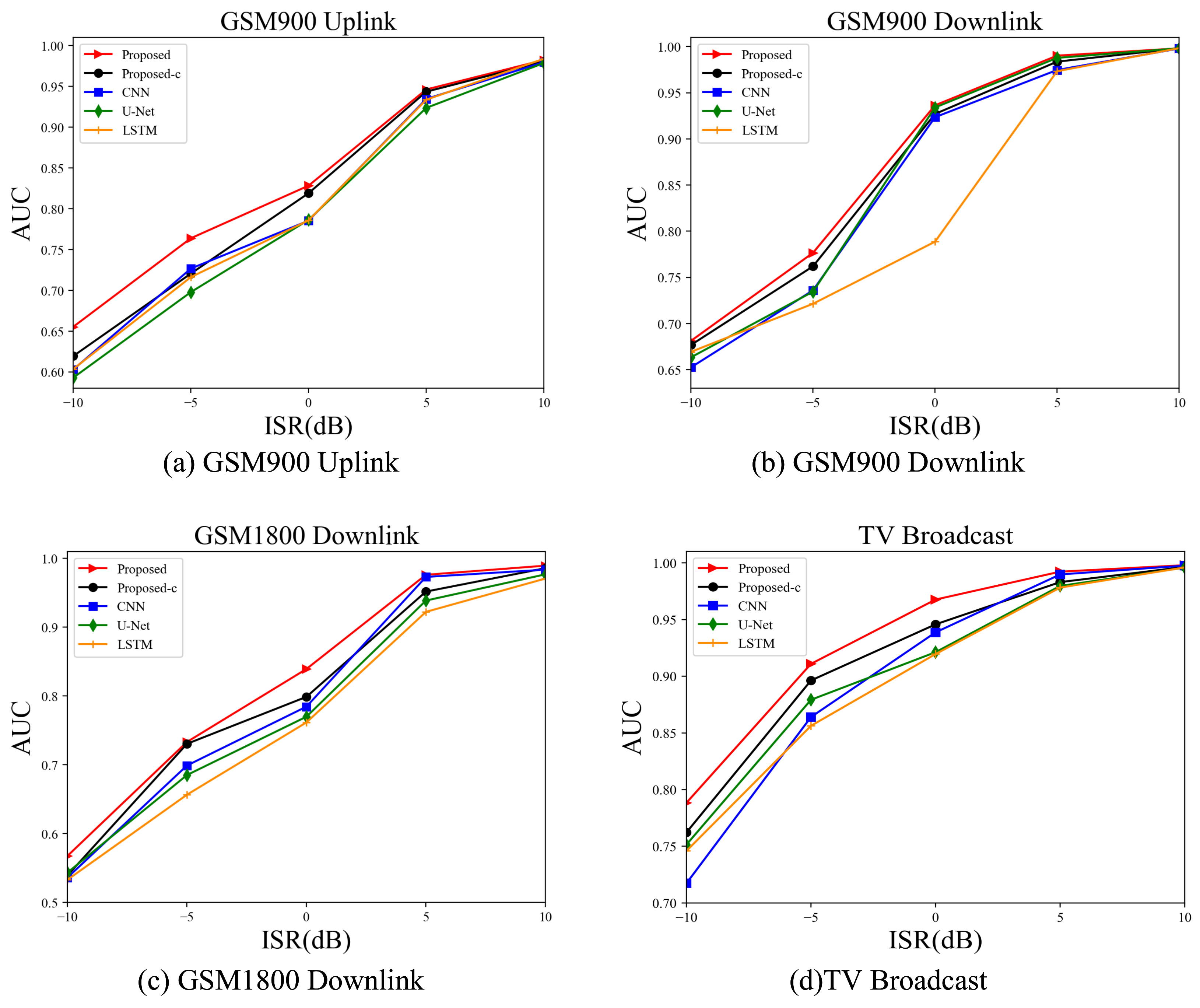
The anomaly detection performance under ISR ∈ [−10 dB, 10 dB] is investigated by varying the intensity of the anomaly data. The algorithm performance experiments in the GSM900 UL band, GSM900 DL, GSM1800 DL, and TV bands. The comparison models include LSTM, CNN, U-Net, Proposed-C, and Proposed models, and Figure 8 shows the variation of AUC values with ISR for each model.

Analysis of Figure 8 shows that the ISR increases with the intensity of the anomalous data, and the algorithm anomaly detection accuracy increases. The duration of the presence of anomalous interference, the bandwidth, and the location of the frequencies where it occurs all impact the anomaly detection performance of the algorithm. In the environment of high ISR, the anomaly exists for a long time and with high energy, and the anomalous interference changes the spectrum data significantly and is less difficult to detect. As the ISR decreases, the anomaly existence time becomes shorter, the energy decreases, and part of the anomalous interference may be submerged in the intense signal spectrum. Short-time anomalies and narrow-bandwidth anomalous interference make the difference between the true and predicted spectrum minimal and difficult to detect, which is the main reason for the degradation of anomaly detection performance.

Since the anomaly detection performance of the model is directly related to the prediction performance of the model. It has been verified in the above experiments that the prediction model based on multiple time scales proposed in this paper has higher prediction accuracy compared to other models. Correspondingly, it shows a superior anomaly detection performance. We are taking the GSM900UL band as an example; when ISR = −10 dB, the anomaly detection performance of the Proposed model is improved by about 8% compared with the CNN model and about 5.7% compared with the LSTM model, which fully illustrates the impact of the prediction performance of the illustrated model on the detection results. However, the anomaly detection performance of each model is similar when ISR = 10 dB and almost all of them can achieve perfect anomaly detection. It can be found that when the ISR is negative, the improvement of anomaly detection accuracy brought by prediction accuracy is more obvious.

In addition, comparing the anomaly detection performance of Proposed and Proposed-C, we know that the inclusion of multi-timescale data successfully improves the anomaly detection performance of the model. The performance improvement is evident at low ISR, about 5.8% and 5% in GSM900UL and GSM1800DL bands, respectively, when ISR = −10 dB. Compared with the existing algorithm models, the algorithm in this paper effectively utilizes the multi-timescale information to improve the model prediction performance, which is more efficient in anomaly detection and the performance is relatively less affected by the ISR variation.

The paper explores the prediction performance of the model, the appropriate discriminative function, and the anomaly detection performance of the model through three experiments, respectively. By analyzing and summarizing the experimental results, we verify the effectiveness and rationality of the anomaly detection framework proposed in this paper. If analyzed in terms of network structure, the model can achieve the fusion and selection of multiple features, improving model performance. The algorithm in this paper can effectively utilize historical data of different time scales, which enhances the anomaly detection performance.

5. Conclusions

This study aims to investigate the electromagnetic spectrum anomaly detection algorithm. We propose an algorithmic framework for detecting spectral anomalies using deep learning techniques. The framework consists of two parts: spectral prediction and anomaly detection. We analyze historical data at different time scales and construct a dataset containing data at multi-timescales using a sliding window approach. The prediction model contains two different feature extraction modules capable of extracting the data’s convolutional features and temporal features. The model is trained with normal data at multiple time scales to enable the model to predict the spectrum with high accuracy. The discriminant function is determined experimentally, and the difference between the predicted and received data is calculated to distinguish the spectral anomalies. We combined real-world spectral data and simulation-generated anomaly data to conduct experiments in several frequency bands and obtained good prediction and anomaly detection results. In future, we intend to continue improving the model structure by combining the physical characteristics of the spectral data and testing the model’s performance for detecting more kinds of abnormal states.