Numerical Integration-Based Performance Analysis of Amplitude-Comparison Monopulse Algorithm in Correlated Noise

Abstract

In this paper, the performance analysis of the amplitude-comparison monopulse (ACM) algorithm under a correlated noise effect is dealt with. The noise received by a monopulse antenna is caused by various sources, such as jamming, multipath, clutter, and thermal noise. The noise variables caused by these noise sources may be correlated with each other when received by the antenna elements. We explicitly analyzed the angle estimation performance of the monopulse algorithm when a correlated noise is received by deriving the probability density function (PDF) of the channel noise variables. In this process, correlation coefficients between noise variables received by antenna elements are defined, and variance and correlation coefficients of channel noise variables are derived. The performance of the angle estimation is analyzed by calculating the root mean square error (RMSE) for various variances and correlation coefficients of the received noise variables. The expectation operation required for calculating the RMSE is performed via numerical integration. Consequently, the analytically derived RMSE results show excellent agreements with the Monte Carlo simulation-based RMSE result, and it is confirmed that the RMSE decreases as the correlation coefficient between the received noise variables increases. When the SNR is high and on-axis, the RMSE decreases by 20% whenever the correlation coefficient between the reception noise variables increases by 0.2.

1. Introduction

Radar can perform the functions of measuring the distance, angle, and speed of the target. The angle information of the target is obtained by measuring the direction of the radar pointing toward the target. The function of the radar tracking the target is implemented by inputting the estimated angle error to the servo system that controls the pointing direction of the radar. In general, lobe switching, conical scan, and monopulse systems are used to calculate the estimated angle error, and these radars are tracking radars. An amplitude-comparison monopulse (ACM) radar can accurately measure the estimated angle error of the target with only one pulse (monopulse). An ACM radar measures the target echo signal voltages through multiple squinted beams [1]. The voltages of the received signal, obtained by using several squinted beams, are input to the difference channels and the sum channel, and the tracking error voltage can be obtained through the ratio of the outputs of these channels [2,3,4]. Through these tracking error voltages, the antenna positioning servo motor is controlled so that the azimuth tracking error and elevation tracking error become zero [5,6].

Estimating various parameters of a radar target is affected by various noises. In the ACM, the noise has a great influence on the ability to estimate the angular position of the target. In some cases, noises can become an obstacle to the precise tracking of the target. In [7,8,9,10,11,12,13], a performance analysis considering the deviation of the estimated angle of the target expressed as measurement noise and a performance analysis by internal error were conducted. In addition, various monopulse algorithms have been proposed to improve the angle estimation accuracy in the presence of noise and interfering signals.

In [7], some facts related to the angle measurement precision of monopulse radar are analyzed. It is explained that the important factors related to angle measurement accuracy of monopulse radar are receiver output noise and squint angle. In relation to internal noise including output noise, a study was conducted to analyze the influence of internal errors. In [8], four main types of monopulse receivers are analyzed with respect to the influence of internal error sources on the resulting measurement accuracy. In [9], the authors presented the least-squares-based monopulse algorithm and a novel covariance prediction equation. The proposed method can accurately predict the performance of the monopulse algorithm. In [10], the effect on the angle estimation ability of monopulse radar when amplitude and phase are not constant was studied. In addition, various monopulse algorithms are proposed to reduce the effects of various noises. Noise jamming is an effective jamming technique to degrade a radar’s capacity to estimate angles. This corresponds to artificial noise caused by an external source. Adaptive digital beamforming was proposed in [11] to maintain the target angle estimation accuracy of the monopulse in the jamming effect. Conventionally, adaptive beamforming is proposed to suppress unwanted signals such as noise, but this technique causes beam distortion. The new monopulse algorithm proposed in [12] acquires the target angle without distorting the beam shape. In addition, in order for the monopulse radar seeker to increase the angle measurement accuracy in the low signal-to-noise ratio (SNR) environment, the authors of [13] proposed an estimation algorithm based on the Bayesian framework.

In previous studies [14,15], the MSE of the ACM direction-of-arrival (DOA) estimated angle was expressed as an analytic expression using the Taylor approximation and was compared with the Monte Carlo method. The analytical expressions proposed in [14,15] are highly computationally efficient. The final expressions quantifying the MSE of the monopulse algorithm in the previous studies are very long and complicated and are not intuitive. In addition, to take higher-order nonlinearities into account, higher-order Taylor expansion should be employed, which makes the expression of the MSE much more complicated. In [16,17,18,19], the output of the ACM radar under the influence of noise is analyzed via probability characteristics. In [16], the monopulse ratio (MR) is regarded as a random variable and the probability density function (PDF) of the MR is derived. In [17], the joint PDF is mathematically derived by dividing the MR into real and imaginary parts for each channel, and the result is used to develop marginal density for the special case of the real correlation of the channels. In [18], the conditional mean and conditional variance are derived and quantified as threshold levels as well as the SNR. In [19], the theoretical expression derived from [18] is verified through simulation, and a detailed description is given to quantify the angle measurement performance under the multi-jamming effect. The PDF of the MR presented in [16,17] is derived for the general case considering the correlation of noise, but it is difficult to use due to the complexity of the formula. Moreover, in [18,19], it is difficult to analyze the angle estimation performance because the mean and variance of the MR for the SNR, not the estimated angle, are shown as results. Previous related studies analyzed the MR when the difference channel and sum channel of the MR are correlated with each other. We further analyzed the root mean square error (RMSE) of the estimated angle when the measurement noise correlated by an external noise source is received via a monopulse antenna.

In this paper, the RMSE of the estimated angle of the ACM algorithm is analytically derived using the PDF considering the probabilistic characteristics of the noise random variables, and the RMSE is calculated using numerical integration. The received noise random variables are the measurement noise received by the antenna elements. We analyzed the angle estimation performance by considering the correlation between these noise variables. The expectations of the channel noise variables are obtained as a linear combination of the expectations of the measured noise variables, but the variance of the channel noise variables requires additional consideration of the covariance terms as well as the variance of the measured noise variables. We describe a monopulse antenna with four antenna elements for azimuth and elevation measurements. Therefore, by defining six correlation coefficients between the four received noise variables, the variance and correlation coefficients of the channel noise are derived. The variances and correlation coefficients obtained in this way are used as arguments of the bivariate Gaussian PDF for the channel noise variables. Then, the RMSE is calculated by performing the integration considering only the main occurrence range of the channel noise.

In Section 2.1, the equations for the signals received by the four antenna elements are defined. In Section 2.2, the definition of the channel noise variables and their expectations and variances are derived. In Section 2.3, an analytical expression of the RMSE of the estimated angle is described. In Section 2.4, the Monte Carlo simulation-based RMSE to verify the analytically derived RMSE is presented and a method for generating correlated noise variables is described. In Section 3, the analytical RMSEs are verified by comparing them with the Monte Carlo simulation-based RMSE, and the RMSE results for the correlation coefficient change between the received noise variables are presented. In addition, the correlation coefficient results of the channel noise variables to the ratio of variances of the received noise variables are presented, and the RMSE results are presented for the difference channel SNR and the sum channel SNR. In Section 4, the validity of this study is emphasized through comparison with the performance analysis method proposed in related studies. In Section 5, conclusions are drawn by analyzing the results obtained in Section 3.

2. Methodology

2.1. Definition of Received Signals for Monopulse Radar

Monopulse radar is a tracking radar and measures the angle (tracking error) through only one pulse. The angle estimation of monopulse radar consists of a phase-comparison method and an amplitude-comparison method. In this paper, it is assumed that the amplitude-comparison monopulse radar have four feed horns and three channels (azimuth difference channel, elevation difference channel, sum channel) [1,2,3]. ACM radar receives an incident signal using squinted beams. Figure 1 shows the antenna array plane of the monopulse radar and incident angle of the target. In this figure, ${\theta }_T$ is the angle of incidence between the target and the antenna boresight; A, B, C, and D are antenna elements; and ${\theta }_{\mathrm{azi}}$ and ${\theta }_{\mathrm{ele}}$ are the azimuth and elevation tracking errors for the target, respectively.

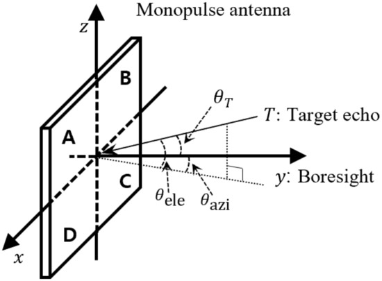
Figure 1. Monopulse antenna array and target angle error.

In Figure 1, the positive azimuth direction is defined as a direction that increases in the positive x-axis direction with respect to the boresight y-axis, and the negative azimuth direction is defined as a direction that increases in the negative x-axis direction. Similarly, the positive elevation direction is defined as a direction that increases along the positive z-axis with respect to the y-axis, and the negative elevation direction is defined as a direction that increases along the negative z-axis.

The target is a non-fluctuating single target, and when the radar is tracking the target, the target’s line of sight (LOS) and antenna boresight are nearly aligned. Therefore, the target echo signals incident on the antenna elements are all modeled to have the same amplitude envelope [20]. The signals received by the antenna elements are:

$$\begin{array}{c}{x}_{\mathrm{A}}=G_{\mathrm{A}}\left({\theta }_T\right)T+n_{\mathrm{A}}\hfill \\ \\ x_{\mathrm{B}}=G_{\mathrm{B}}\left({\theta }_T\right)T+n_{\mathrm{B}}\hfill \\ \\ x_{\mathrm{C}}=G_{\mathrm{C}}\left({\theta }_T\right)T+n_{\mathrm{C}}\hfill \\ \\ x_{\mathrm{D}}=G_{\mathrm{D}}\left({\theta }_T\right)T+n_{\mathrm{D}},\hfill \end{array}$$

(1)

where T is the voltage amplitude of the target echo; $G_{\mathrm{A}}$, $G_{\mathrm{B}}$, $G_{\mathrm{C}}$, and $G_{\mathrm{D}}$ are the voltage gains; and $n_{\mathrm{A}}$, $n_{\mathrm{B}}$, $n_{\mathrm{C}}$, and $n_{\mathrm{D}}$ are the received noise variables, respectively.

The received noise is caused by several environmental variables (jamming, external sources, interference, and propagation effects). Typically, thermal noise exists inside the antenna element and receiver. Thermal noise random variables present in antenna elements are not correlated with each other. However, noise random variables of antenna elements present by noise jamming or unresolved targets are correlated with each other [1]. In Figure 2, the correlation between the received noise variables of the antenna elements is shown.

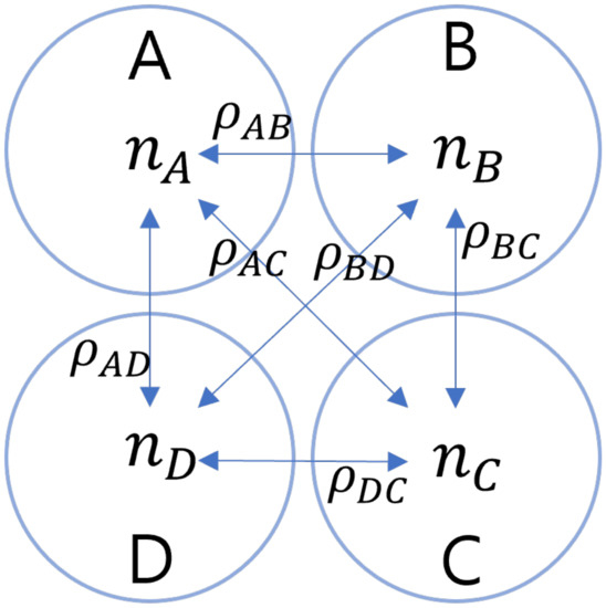
Figure 2. Correlation coefficients between the noise variables received by the four antenna elements.

In Figure 2, ${\rho }_{ij}$ denotes a correlation coefficient between $n_i$ and $n_j$. The definition of the correlation coefficient is as follows [21]:

$$\begin{array}{ccc}\hfill {\rho }_{ij}=\frac{\mathrm{cov}\left[n_i,n_j\right]}{{\sigma }_i{\sigma }_j}& \hfill & \hfill \left(i\ne j:\forall i,j\in \left\{\mathrm{A},\mathrm{B},\mathrm{C},\mathrm{D}\right\}\right),\end{array}$$

(2)

where $\mathrm{cov}\left[n_i,n_j\right]$ is the covariance of $n_i$ and $n_j$, and ${\sigma }_i$ and ${\sigma }_j$ are the standard deviations of $n_i$ and $n_j$.

2.2. Definition of Channel Noise Variables for Receiver of Monopulse Radar

The channels consist of the azimuth difference channel (${\Delta }_{\mathrm{azi}}$), the elevation difference channel (${\Delta }_{\mathrm{ele}}$), and the sum channel ($\Sigma$). The target echo signal is input to the sum channel and difference channels, and the tracking error is estimated through the output of these channels. In Figure 3, a comparator for obtaining the elevation tracking error and the azimuth tracking error is shown. The elevation tracking error and azimuth tracking error are input to the closed-loop servo system so that the antenna boresight can be directed to the moving target [5,6].

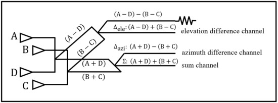
Figure 3. Monopulse comparator [5].

In Figure 3, the azimuth difference channel can be obtained through (A + D) − (B + C), the elevation difference channel can be obtained through (A + B) − (D + C), and the sum channel can be obtained through (A + B) + (C + D). Using (1), the outputs of the channels are as follows:

$$\begin{array}{c}{\Delta }_{\mathrm{azi}}\stackrel{\Delta }{=}{x}_{\mathrm{A}}+x_{\mathrm{D}}-\left(x_{\mathrm{B}}+x_{\mathrm{C}}\right)\hfill \\ =T\left[G_{\mathrm{A}}\left({\theta }_T\right)+G_{\mathrm{D}}\left({\theta }_T\right)-G_{\mathrm{B}}\left({\theta }_T\right)-G_{\mathrm{C}}\left({\theta }_T\right)\right]+n_{\mathrm{A}}+n_{\mathrm{D}}-n_{\mathrm{B}}-n_{\mathrm{C}}\hfill \end{array}$$

(3)

$$\begin{array}{c}{\Delta }_{\mathrm{ele}}\stackrel{\Delta }{=}{x}_{\mathrm{A}}+x_{\mathrm{B}}-\left(x_{\mathrm{C}}+x_{\mathrm{D}}\right)\hfill \\ =T\left[G_{\mathrm{A}}\left({\theta }_T\right)+G_{\mathrm{B}}\left({\theta }_T\right)-G_{\mathrm{C}}\left({\theta }_T\right)-G_{\mathrm{D}}\left({\theta }_T\right)\right]+n_{\mathrm{A}}+n_{\mathrm{B}}-n_{\mathrm{C}}-n_{\mathrm{D}}\hfill \end{array}$$

(4)

$$\begin{array}{c}\Sigma \stackrel{\Delta }{=}{x}_{\mathrm{A}}+x_{\mathrm{B}}+x_{\mathrm{C}}+x_{\mathrm{D}}\hfill \\ =T\left[G_{\mathrm{A}}\left({\theta }_T\right)+G_{\mathrm{B}}\left({\theta }_T\right)+G_{\mathrm{C}}\left({\theta }_T\right)+G_{\mathrm{D}}\left({\theta }_T\right)\right]+n_{\mathrm{A}}+n_{\mathrm{B}}+n_{\mathrm{C}}+n_{\mathrm{D}}.\hfill \end{array}$$

(5)

Here, the outputs of the channels are a linear combination of the received signals of the antenna elements. Therefore, if the noise generated inside the receiver is ignored, the channel noise variables can be expressed as a linear combination of the received noise variables, i.e.,

$$\begin{array}{c}{n}_{\mathrm{azi}}=n_{\mathrm{A}}+n_{\mathrm{D}}-n_{\mathrm{B}}-n_{\mathrm{C}}\hfill \\ \\ n_{\mathrm{ele}}=n_{\mathrm{A}}+n_{\mathrm{B}}-n_{\mathrm{C}}-n_{\mathrm{D}}\hfill \\ \\ n_{\mathrm{sum}}=n_{\mathrm{A}}+n_{\mathrm{B}}+n_{\mathrm{C}}+n_{\mathrm{D}}.\hfill \end{array}$$

(6)

Similarly, the voltage gains can be simplified as

$$\begin{array}{c}{G}_{\mathrm{azi}}\left(\theta \right)=G_{\mathrm{A}}\left(\theta \right)+G_{\mathrm{D}}\left(\theta \right)-G_{\mathrm{B}}\left(\theta \right)-G_{\mathrm{C}}\left(\theta \right)\hfill \\ \\ G_{\mathrm{ele}}\left(\theta \right)=G_{\mathrm{A}}\left(\theta \right)+G_{\mathrm{B}}\left(\theta \right)-G_{\mathrm{C}}\left(\theta \right)-G_{\mathrm{D}}\left(\theta \right)\hfill \\ \\ G_{\mathrm{sum}}\left(\theta \right)=G_{\mathrm{A}}\left(\theta \right)+G_{\mathrm{B}}\left(\theta \right)+G_{\mathrm{C}}\left(\theta \right)+G_{\mathrm{D}}\left(\theta \right),\hfill \end{array}$$

(7)

where $G_{\mathrm{azi}}$, $G_{\mathrm{ele}}$, and $G_{\mathrm{sum}}$ denote azimuth difference pattern gain, elevation difference pattern gain, and sum pattern gain, respectively.

Through (6) and (7), the channel outputs are summarized as follows:

$${\Delta }_{\mathrm{azi}}=G_{\mathrm{azi}}\left({\theta }_T\right)T+n_{\mathrm{azi}}$$

(8)

$${\Delta }_{\mathrm{ele}}=G_{\mathrm{ele}}\left({\theta }_T\right)T+n_{\mathrm{ele}}$$

(9)

$$\Sigma =G_{\mathrm{sum}}\left({\theta }_T\right)T+n_{\mathrm{sum}}.$$

(10)

In general, the received noise variables are modeled with a Gaussian distribution:

$$\begin{array}{c}{n}_{\mathrm{A}}\sim \mathcal{N}\left(0,{\sigma }_{\mathrm{A}}^2\right)\hfill \\ \\ n_{\mathrm{B}}\sim \mathcal{N}\left(0,{\sigma }_{\mathrm{B}}^2\right)\hfill \\ \\ n_{\mathrm{C}}\sim \mathcal{N}\left(0,{\sigma }_{\mathrm{C}}^2\right)\hfill \\ \\ n_{\mathrm{D}}\sim \mathcal{N}\left(0,{\sigma }_{\mathrm{D}}^2\right).\hfill \end{array}$$

(11)

Here, all received noise variables are set to have zero mean and standard deviations of ${\sigma }_{\mathrm{A}}$, ${\sigma }_{\mathrm{B}}$, ${\sigma }_{\mathrm{C}}$, and ${\sigma }_{\mathrm{D}}$. Because the random variables defined in (6) are the sum of correlated Gaussian random variables, $n_{\mathrm{azi}}$, $n_{\mathrm{ele}}$, and $n_{\mathrm{sum}}$ are also Gaussian random variables [22]:

$$\begin{array}{c}{n}_{\mathrm{azi}}\sim \mathcal{N}\left({\mu }_{\mathrm{azi}},{\sigma }_{\mathrm{azi}}^2\right)\hfill \\ \\ n_{\mathrm{ele}}\sim \mathcal{N}\left({\mu }_{\mathrm{ele}},{\sigma }_{\mathrm{ele}}^2\right)\hfill \\ \\ n_{\mathrm{sum}}\sim \mathcal{N}\left({\mu }_{\mathrm{sum}},{\sigma }_{\mathrm{sum}}^2\right).\hfill \end{array}$$

(12)

The expectations of the channel noise variables are given as the sum of the expectations of the receive noise variables:

$${\mu }_{\mathrm{azi}}=\mathrm{E}\left[n_{\mathrm{A}}+n_{\mathrm{D}}-n_{\mathrm{B}}-n_{\mathrm{C}}\right]={\mu }_{\mathrm{A}}+{\mu }_{\mathrm{D}}-{\mu }_{\mathrm{B}}-{\mu }_{\mathrm{C}}=0$$

(13)

$${\mu }_{\mathrm{ele}}=\mathrm{E}\left[n_{\mathrm{A}}+n_{\mathrm{B}}-n_{\mathrm{C}}-n_{\mathrm{D}}\right]={\mu }_{\mathrm{A}}+{\mu }_{\mathrm{D}}-{\mu }_{\mathrm{B}}-{\mu }_{\mathrm{C}}=0$$

(14)

$${\mu }_{\mathrm{sum}}=\mathrm{E}\left[n_{\mathrm{A}}+n_{\mathrm{B}}+n_{\mathrm{C}}+n_{\mathrm{D}}\right]={\mu }_{\mathrm{A}}+{\mu }_{\mathrm{B}}+{\mu }_{\mathrm{C}}+{\mu }_{\mathrm{D}}=0.$$

(15)

The variances of the channel noise variables consist of the variance and covariance terms of the receive noise variables:

$$\begin{array}{c}{\sigma }_{\mathrm{azi}}^2=\mathrm{E}\left[{\left(n_{\mathrm{azi}}-{\mu }_{\mathrm{azi}}\right)}^2\right]=\mathrm{E}\left[{\left(n_{\mathrm{A}}+n_{\mathrm{D}}-n_{\mathrm{B}}-n_{\mathrm{C}}\right)}^2\right]\hfill \\ =\mathrm{var}\left[n_{\mathrm{A}}\right]+\mathrm{var}\left[n_{\mathrm{B}}\right]+\mathrm{var}\left[n_{\mathrm{C}}\right]+\mathrm{var}\left[n_{\mathrm{D}}\right]\hfill \\ +2\left(\mathrm{cov}\left[n_{\mathrm{A}},n_{\mathrm{D}}\right]-\mathrm{cov}\left[n_{\mathrm{A}},n_{\mathrm{B}}\right]-\mathrm{cov}\left[n_{\mathrm{A}},n_{\mathrm{C}}\right]-\mathrm{cov}\left[n_{\mathrm{D}},n_{\mathrm{B}}\right]-\mathrm{cov}\left[n_{\mathrm{D}},n_{\mathrm{C}}\right]+\mathrm{cov}\left[n_{\mathrm{B}},n_{\mathrm{C}}\right]\right)\hfill \\ ={\sigma }_{\mathrm{A}}^2+{\sigma }_{\mathrm{B}}^2+{\sigma }_{\mathrm{C}}^2+{\sigma }_{\mathrm{D}}^2\hfill \\ +2\left({\rho }_{\mathrm{AD}}{\sigma }_{\mathrm{A}}{\sigma }_{\mathrm{D}}-{\rho }_{\mathrm{AB}}{\sigma }_{\mathrm{A}}{\sigma }_{\mathrm{B}}-{\rho }_{\mathrm{AC}}{\sigma }_{\mathrm{A}}{\sigma }_C-{\rho }_{\mathrm{DB}}{\sigma }_{\mathrm{D}}{\sigma }_{\mathrm{B}}-{\rho }_{\mathrm{DC}}{\sigma }_{\mathrm{D}}{\sigma }_{\mathrm{C}}+{\rho }_{\mathrm{BC}}{\sigma }_{\mathrm{B}}{\sigma }_{\mathrm{C}}\right)\hfill \end{array}$$

(16)

$$\begin{array}{c}{\sigma }_{\mathrm{ele}}^2=\mathrm{E}\left[{\left(n_{\mathrm{ele}}-{\mu }_{\mathrm{ele}}\right)}^2\right]=\mathrm{E}\left[{\left(n_{\mathrm{A}}+n_{\mathrm{B}}-n_{\mathrm{C}}-n_{\mathrm{D}}\right)}^2\right]\hfill \\ =\mathrm{var}\left[n_{\mathrm{A}}\right]+\mathrm{var}\left[n_{\mathrm{B}}\right]+\mathrm{var}\left[n_{\mathrm{C}}\right]+\mathrm{var}\left[n_{\mathrm{D}}\right]\hfill \\ +2\left(\mathrm{cov}\left[n_{\mathrm{A}},n_{\mathrm{B}}\right]-\mathrm{cov}\left[n_{\mathrm{A}},n_{\mathrm{D}}\right]-\mathrm{cov}\left[n_{\mathrm{A}},n_{\mathrm{C}}\right]-\mathrm{cov}\left[n_{\mathrm{B}},n_{\mathrm{D}}\right]-\mathrm{cov}\left[n_{\mathrm{B}},n_{\mathrm{C}}\right]+\mathrm{cov}\left[n_{\mathrm{C}},n_{\mathrm{D}}\right]\right)\hfill \\ ={\sigma }_{\mathrm{A}}^2+{\sigma }_{\mathrm{B}}^2+{\sigma }_{\mathrm{C}}^2+{\sigma }_{\mathrm{D}}^2\hfill \\ +2\left({\rho }_{\mathrm{AB}}{\sigma }_{\mathrm{A}}{\sigma }_{\mathrm{B}}-{\rho }_{\mathrm{AD}}{\sigma }_{\mathrm{A}}{\sigma }_{\mathrm{D}}-{\rho }_{\mathrm{AC}}{\sigma }_{\mathrm{A}}{\sigma }_C-{\rho }_{\mathrm{BD}}{\sigma }_{\mathrm{B}}{\sigma }_{\mathrm{D}}-{\rho }_{\mathrm{BC}}{\sigma }_{\mathrm{B}}{\sigma }_{\mathrm{C}}+{\rho }_{\mathrm{CD}}{\sigma }_{\mathrm{C}}{\sigma }_{\mathrm{D}}\right)\hfill \end{array}$$

(17)

$$\begin{array}{c}{\sigma }_{\mathrm{sum}}^2=\mathrm{E}\left[{\left(n_{\mathrm{sum}}-{\mu }_{\mathrm{sum}}\right)}^2\right]=\mathrm{E}\left[{\left(n_{\mathrm{A}}+n_{\mathrm{B}}+n_{\mathrm{C}}+n_{\mathrm{D}}\right)}^2\right]\hfill \\ =\mathrm{var}\left[n_{\mathrm{A}}\right]+\mathrm{var}\left[n_{\mathrm{B}}\right]+\mathrm{var}\left[n_{\mathrm{C}}\right]+\mathrm{var}\left[n_{\mathrm{D}}\right]\hfill \\ +2\left(\mathrm{cov}\left[n_{\mathrm{A}},n_{\mathrm{D}}\right]+\mathrm{cov}\left[n_{\mathrm{A}},n_{\mathrm{B}}\right]+\mathrm{cov}\left[n_{\mathrm{A}},n_{\mathrm{C}}\right]+\mathrm{cov}\left[n_{\mathrm{D}},n_{\mathrm{B}}\right]+\mathrm{cov}\left[n_{\mathrm{D}},n_{\mathrm{C}}\right]+\mathrm{cov}\left[n_{\mathrm{B}},n_{\mathrm{C}}\right]\right)\hfill \\ ={\sigma }_{\mathrm{A}}^2+{\sigma }_{\mathrm{B}}^2+{\sigma }_{\mathrm{C}}^2+{\sigma }_{\mathrm{D}}^2\hfill \\ +2\left({\rho }_{\mathrm{AD}}{\sigma }_{\mathrm{A}}{\sigma }_{\mathrm{D}}+{\rho }_{\mathrm{AB}}{\sigma }_{\mathrm{A}}{\sigma }_{\mathrm{B}}+{\rho }_{\mathrm{AC}}{\sigma }_{\mathrm{A}}{\sigma }_C+{\rho }_{\mathrm{DB}}{\sigma }_{\mathrm{D}}{\sigma }_{\mathrm{B}}+{\rho }_{\mathrm{DC}}{\sigma }_{\mathrm{D}}{\sigma }_{\mathrm{C}}+{\rho }_{\mathrm{BC}}{\sigma }_{\mathrm{B}}{\sigma }_{\mathrm{C}}\right).\hfill \end{array}$$

(18)

The covariances between the channel noises are obtained as

$$\begin{array}{c}\mathrm{cov}\left[n_{\mathrm{azi}},n_{\mathrm{sum}}\right]\hfill \\ =\mathrm{E}\left[\left(n_{\mathrm{azi}}-{\mu }_{\mathrm{azi}}\right)\left(n_{\mathrm{sum}}-{\mu }_{\mathrm{sum}}\right)\right]\hfill \\ =\mathrm{E}\left[\left(n_{\mathrm{A}}+n_{\mathrm{D}}-n_{\mathrm{B}}-n_{\mathrm{C}}\right)\left(n_{\mathrm{A}}+n_{\mathrm{B}}+n_{\mathrm{C}}+n_{\mathrm{D}}\right)\right]\hfill \\ =\mathrm{var}\left[n_{\mathrm{A}}\right]+\mathrm{var}\left[n_{\mathrm{D}}\right]-\mathrm{var}\left[n_{\mathrm{B}}\right]-\mathrm{var}\left[n_{\mathrm{C}}\right]+2\mathrm{cov}\left[n_{\mathrm{A}},n_{\mathrm{D}}\right]-2\mathrm{cov}\left[n_{\mathrm{B}},n_{\mathrm{C}}\right]\hfill \\ ={\sigma }_{\mathrm{A}}^2+{\sigma }_{\mathrm{D}}^2-{\sigma }_{\mathrm{B}}^2-{\sigma }_{\mathrm{C}}^2+2{\rho }_{\mathrm{AD}}{\sigma }_{\mathrm{A}}{\sigma }_{\mathrm{D}}-2{\rho }_{\mathrm{BC}}{\sigma }_{\mathrm{B}}{\sigma }_{\mathrm{C}}\hfill \end{array}$$

(19)

$$\begin{array}{c}\mathrm{cov}\left[n_{\mathrm{ele}},n_{\mathrm{sum}}\right]\hfill \\ =\mathrm{E}\left[\left(n_{\mathrm{ele}}-{\mu }_{\mathrm{ele}}\right)\left(n_{\mathrm{sum}}-{\mu }_{\mathrm{sum}}\right)\right]\hfill \\ =\mathrm{E}\left[\left(n_{\mathrm{A}}+n_{\mathrm{B}}-n_{\mathrm{C}}-n_{\mathrm{D}}\right)\left(n_{\mathrm{A}}+n_{\mathrm{B}}+n_{\mathrm{C}}+n_{\mathrm{D}}\right)\right]\hfill \\ =\mathrm{var}\left[n_{\mathrm{A}}\right]+\mathrm{var}\left[n_{\mathrm{B}}\right]-\mathrm{var}\left[n_{\mathrm{C}}\right]-\mathrm{var}\left[n_{\mathrm{D}}\right]+2\mathrm{cov}\left[n_{\mathrm{A}},n_{\mathrm{B}}\right]-2\mathrm{cov}\left[n_{\mathrm{C}},n_{\mathrm{D}}\right]\hfill \\ ={\sigma }_{\mathrm{A}}^2+{\sigma }_{\mathrm{B}}^2-{\sigma }_{\mathrm{C}}^2-{\sigma }_{\mathrm{D}}^2+2{\rho }_{\mathrm{AB}}{\sigma }_{\mathrm{A}}{\sigma }_{\mathrm{B}}-2{\rho }_{\mathrm{CD}}{\sigma }_{\mathrm{C}}{\sigma }_{\mathrm{D}}.\hfill \end{array}$$

(20)

Note that the covariances of the channel noise variables do not consider the correlation coefficients of all received noise variables, but only two correlation coefficient terms. Moreover, in (19) and (20), it can be seen that the channel noise variables are linear combinations of the received noise variables, but there is no correlation between the channel noise variables under certain conditions.

2.3. Analytical Expression for Performance Analysis of Amplitude-Comparison Monopulse Radar

The correlation coefficient between the channel noise variables can be obtained using (16)–(20):

$${\rho }_{\mathrm{azi}}{,}_{\mathrm{sum}}=\frac{\mathrm{cov}\left[n_{\mathrm{azi}},n_{\mathrm{sum}}\right]}{{\sigma }_{\mathrm{azi}}{\sigma }_{\mathrm{sum}}}$$

(21)

$${\rho }_{\mathrm{ele}}{,}_{\mathrm{sum}}=\frac{\mathrm{cov}\left[n_{\mathrm{ele}},n_{\mathrm{sum}}\right]}{{\sigma }_{\mathrm{ele}}{\sigma }_{\mathrm{sum}}}.$$

(22)

Equations (23) and (24) are the estimated angle equations of the monopulse algorithm [1]:

$${\widehat{\theta }}_{\mathrm{azi}}=\frac{{\theta }_{3\mathrm{dB}}}{k_{\mathrm{m}}}\frac{{\Delta }_{\mathrm{azi}}}{\Sigma }=\frac{{\theta }_{3\mathrm{dB}}}{k_{\mathrm{m}}}\frac{G_{\mathrm{azi}}\left({\theta }_T\right)T+n_{\mathrm{azi}}}{G_{\mathrm{sum}}\left({\theta }_T\right)T+n_{\mathrm{sum}}}$$

(23)

$${\widehat{\theta }}_{\mathrm{ele}}=\frac{{\theta }_{3\mathrm{dB}}}{k_{\mathrm{m}}}\frac{{\Delta }_{\mathrm{ele}}}{\Sigma }=\frac{{\theta }_{3\mathrm{dB}}}{k_{\mathrm{m}}}\frac{G_{\mathrm{ele}}\left({\theta }_T\right)T+n_{\mathrm{ele}}}{G_{\mathrm{sum}}\left({\theta }_T\right)T+n_{\mathrm{sum}}}.$$

(24)

where ${\widehat{\theta }}_{\mathrm{azi}}$ and ${\widehat{\theta }}_{\mathrm{ele}}$ are the estimated azimuth and estimated elevation, respectively. In addition, $k_{\mathrm{m}}$ and ${\theta }_{3\mathrm{dB}}$ denote the monopulse error slope constant and 3-dB beamwidth of sum pattern, respectively.

The monopulse error slope constant is determined as [1]

$$k_{\mathrm{m}}={\left.{\theta }_{3\mathrm{dB}}\frac{1}{\Sigma \left(\theta \right)}\frac{\partial \Delta \left(\theta \right)}{\partial \theta }\right|}_{\theta =0}.$$

(25)

It is usually convenient to analyze performance in terms of SNR. Thus, in (23) and (24), let the denominator and numerator terms divided by sum channel output of target echo:

$${\widehat{\theta }}_{\mathrm{azi}}=\frac{{\theta }_{3\mathrm{dB}}}{k_{\mathrm{m}}}\frac{\frac{G_{\mathrm{azi}}\left({\theta }_T\right)T}{G_{\mathrm{sum}}\left({\theta }_T\right)T}+\frac{n_{\mathrm{azi}}}{G_{\mathrm{sum}}\left({\theta }_T\right)T}}{1+\frac{n_{\mathrm{sum}}}{G_{\mathrm{sum}}\left({\theta }_T\right)T}}=\frac{{\theta }_{3\mathrm{dB}}}{k_{\mathrm{m}}}\frac{R_{\mathrm{azi}}+u}{1+w}$$

(26)

$${\widehat{\theta }}_{\mathrm{ele}}=\frac{{\theta }_{3\mathrm{dB}}}{k_{\mathrm{m}}}\frac{\frac{G_{\mathrm{ele}}\left({\theta }_T\right)T}{G_{\mathrm{sum}}\left({\theta }_T\right)T}+\frac{n_{\mathrm{ele}}}{G_{\mathrm{sum}}\left({\theta }_T\right)T}}{1+\frac{n_{\mathrm{sum}}}{G_{\mathrm{sum}}\left({\theta }_T\right)T}}=\frac{{\theta }_{3\mathrm{dB}}}{k_{\mathrm{m}}}\frac{R_{\mathrm{ele}}+v}{1+w},$$

(27)

where $R_{\mathrm{azi}}$ and $R_{\mathrm{ele}}$ are the azimuth monopulse ratio and the elevation monopulse ratio of the noise-free signal, respectively. Moreover, u, v, and w are normal distributions with the following characteristic:

$$\begin{array}{c}u\sim \mathcal{N}\left(0,\frac{{\sigma }_{\mathrm{azi}}^2}{{\left(G_{\mathrm{sum}}\left({\theta }_T\right)T\right)}^2}\right)\hfill \\ \\ v\sim \mathcal{N}\left(0,\frac{{\sigma }_{\mathrm{ele}}^2}{{\left(G_{\mathrm{sum}}\left({\theta }_T\right)T\right)}^2}\right)\hfill \\ \\ w\sim \mathcal{N}\left(0,\frac{{\sigma }_{\mathrm{sum}}^2}{{\left(G_{\mathrm{sum}}\left({\theta }_T\right)T\right)}^2}\right).\hfill \end{array}$$

(28)

According to the variance of the three channel noises, three SNRs are defined. The received signal power of the target echo is obtained as the square of the root mean square (RMS) value, and the powers of the channel noises are the variances of the channel noise variables, i.e.,

$$\begin{array}{c}{\mathrm{S}/\mathrm{N}}_{\mathrm{azi}}=\frac{{\left(G_{\mathrm{sum}}\left({\theta }_T\right)T\right)}^2}{2{\sigma }_{\mathrm{azi}}^2}\hfill \\ \\ {\mathrm{S}/\mathrm{N}}_{\mathrm{ele}}=\frac{{\left(G_{\mathrm{sum}}\left({\theta }_T\right)T\right)}^2}{2{\sigma }_{\mathrm{ele}}^2}\hfill \\ \\ {\mathrm{S}/\mathrm{N}}_{\mathrm{sum}}=\frac{{\left(G_{\mathrm{sum}}\left({\theta }_T\right)T\right)}^2}{2{\sigma }_{\mathrm{sum}}^2}.\hfill \end{array}$$

(29)

Here, ${\mathrm{S}/\mathrm{N}}_{\mathrm{azi}}$ and ${\mathrm{S}/\mathrm{N}}_{\mathrm{ele}}$ are defined as difference channel SNR, and ${\mathrm{S}/\mathrm{N}}_{\mathrm{sum}}$ is defined as sum channel SNR.

Root mean square error (RMSE) is one of the measures to measure the accuracy of an estimate. Assuming that the square of the estimated angle error is ergodic [21]. The statistical RMSEs of the estimated azimuth and the estimated elevation are defined as

$$\sqrt{\mathrm{E}\left[{\left({\widehat{\theta }}_{\mathrm{azi}}-{\theta }_{\mathrm{azi}}\right)}^2\right]}={\left({\int }_{-\infty }^{\infty }{\int }_{-\infty }^{\infty }{\left(\frac{{\theta }_{3\mathrm{dB}}}{k_{\mathrm{m}}}\frac{R_{\mathrm{azi}}+u}{1+w}-{\theta }_{\mathrm{azi}}\right)}^2{f}_{u,w}\left(u,w\right)dudw\right)}^{\frac{1}{2}}$$

(30)

$$\sqrt{\mathrm{E}\left[{\left({\widehat{\theta }}_{\mathrm{ele}}-{\theta }_{\mathrm{ele}}\right)}^2\right]}={\left({\int }_{-\infty }^{\infty }{\int }_{-\infty }^{\infty }{\left(\frac{{\theta }_{3\mathrm{dB}}}{k_{\mathrm{m}}}\frac{R_{\mathrm{ele}}+v}{1+w}-{\theta }_{\mathrm{ele}}\right)}^2{f}_{v,w}\left(v,w\right)dvdw\right)}^{\frac{1}{2}},$$

(31)

where $f_{u,w}\left(n_{u,w}\right)$ and $f_{v,w}\left(n_{v,w}\right)$ are bivariate Gaussian joint PDF of $u,w$ and $v,w$, respectively.

The joint PDFs are defined as a function of SNRs and correlation coefficient of channel noise variables:

$$\begin{array}{c}{f}_{u,w}\left(u,w\right)\hfill \\ =\frac{\sqrt{\left({\mathrm{S}/\mathrm{N}}_{\mathrm{azi}}\right)\left({\mathrm{S}/\mathrm{N}}_{\mathrm{sum}}\right)}}{\pi \sqrt{1-{\rho }_{\mathrm{azi},\mathrm{sum}}^2}}\exp \left[-\frac{\left({\mathrm{S}/\mathrm{N}}_{\mathrm{azi}}\right)u^2-2{\rho }_{\mathrm{azi},\mathrm{sum}}\sqrt{\left({\mathrm{S}/\mathrm{N}}_{\mathrm{azi}}\right)\left({\mathrm{S}/\mathrm{N}}_{\mathrm{sum}}\right)}uw+\left({\mathrm{S}/\mathrm{N}}_{\mathrm{sum}}\right)w^2}{\left(1-{\rho }_{\mathrm{azi},\mathrm{sum}}^2\right)}\right]\hfill \end{array}$$

(32)

$$\begin{array}{c}{f}_{v,w}\left(v,w\right)\hfill \\ =\frac{\sqrt{\left({\mathrm{S}/\mathrm{N}}_{\mathrm{ele}}\right)\left({\mathrm{S}/\mathrm{N}}_{\mathrm{sum}}\right)}}{\pi \sqrt{1-{\rho }_{\mathrm{ele},\mathrm{sum}}^2}}\exp \left[-\frac{\left({\mathrm{S}/\mathrm{N}}_{\mathrm{ele}}\right)v^2-2{\rho }_{\mathrm{ele},\mathrm{sum}}\sqrt{\left({\mathrm{S}/\mathrm{N}}_{\mathrm{ele}}\right)\left({\mathrm{S}/\mathrm{N}}_{\mathrm{sum}}\right)}vw+\left({\mathrm{S}/\mathrm{N}}_{\mathrm{sum}}\right)w^2}{\left(1-{\rho }_{\mathrm{ele},\mathrm{sum}}^2\right)}\right].\hfill \end{array}$$

(33)

In order to obtain RMSEs, (30) and (31) should be evaluated using MATLAB’s numerical integration function. The integration intervals are set to a range that is three times the standard deviation.

2.4. Generate Correlated Noise Random Vectors for Monte Carlo Simulations

In this paper, the Monte Carlo simulation is used to verify the analytically derived RMSE described above. That is, ergodicity is confirmed by comparing the results of the numerical integration-based statistical average and the Monte Carlo simulation-based time average in the steady state. Thus, the Monte Carlo simulation is empirically calculated through many repetitions using the original monopulse estimation equation.

The Monte Carlo simulation-based RMSEs are as follows:

$$\sqrt{\mathrm{E}\left[{\left(\widehat{\theta }-\theta \right)}^2\right]}=\sqrt{\frac{1}{N}\sum _{i=1}^N{\left({\widehat{\theta }}_{\left(i\right)}-\theta \right)}^2},$$

(34)

where N denotes the number of repetitions. The estimated angle ${\widehat{\theta }}_{\left(i\right)}$ can be obtained using (23) and (24).

In order to perform a Monte Carlo simulation, we need to generate correlated noise. The noise random vector for the receive noise variables is

$$\mathbf{N}={\left[n_{\mathrm{A}}{n}_{\mathrm{B}}{n}_{\mathrm{C}}{n}_{\mathrm{D}}\right]}^T,$$

(35)

where ${\left(·\right)}^T$ is the transpose operator.

This noise random vector is a Gaussian random vector:

$$\mathbf{N}\sim \mathcal{N}\left({\mathbf{m}}_{\mathbf{N}},{\mathbf{C}}_{\mathbf{N}}\right),$$

(36)

where ${\mathbf{m}}_{\mathbf{N}}$ is the expectation vector and ${\mathbf{C}}_{\mathbf{N}}$ is the covariance matrix of the noise random vector. According to (11), ${\mathbf{m}}_{\mathbf{N}}$ is a zero vector.

Expanding the covariance matrix of the noise random vector is

$$\begin{array}{c}{\mathbf{C}}_{\mathbf{N}}=\mathrm{E}\left[\left(\mathbf{N}-{\mathbf{m}}_{\mathbf{N}}\right){\left(\mathbf{N}-{\mathbf{m}}_{\mathbf{N}}\right)}^T\right]\hfill \\ =\mathrm{E}\left[\left(\begin{array}{cccc}{n}_{\mathrm{A}}^2& n_{\mathrm{A}}{n}_{\mathrm{B}}& n_{\mathrm{A}}{n}_{\mathrm{C}}& n_{\mathrm{A}}{n}_{\mathrm{D}}\\ n_{\mathrm{A}}{n}_{\mathrm{B}}& n_{\mathrm{B}}^2& n_{\mathrm{B}}{n}_{\mathrm{C}}& n_{\mathrm{B}}{n}_{\mathrm{D}}\\ n_{\mathrm{A}}{n}_{\mathrm{C}}& n_{\mathrm{B}}{n}_{\mathrm{C}}& n_{\mathrm{C}}^2& n_{\mathrm{C}}{n}_{\mathrm{D}}\\ n_{\mathrm{A}}{n}_{\mathrm{D}}& n_{\mathrm{B}}{n}_{\mathrm{D}}& n_{\mathrm{C}}{n}_{\mathrm{D}}& n_{\mathrm{D}}^2\end{array}\right)\right]\hfill \\ =\left(\begin{array}{cccc}{\sigma }_{\mathrm{A}}^2& {\rho }_{\mathrm{AB}}{\sigma }_{\mathrm{A}}{\sigma }_{\mathrm{B}}& {\rho }_{\mathrm{AC}}{\sigma }_{\mathrm{A}}{\sigma }_{\mathrm{C}}& {\rho }_{\mathrm{AD}}{\sigma }_{\mathrm{A}}{\sigma }_{\mathrm{D}}\\ {\rho }_{\mathrm{AB}}{\sigma }_{\mathrm{A}}{\sigma }_{\mathrm{B}}& {\sigma }_{\mathrm{B}}^2& {\rho }_{\mathrm{BC}}{\sigma }_{\mathrm{B}}{\sigma }_{\mathrm{C}}& {\rho }_{\mathrm{BD}}{\sigma }_{\mathrm{B}}{\sigma }_{\mathrm{D}}\\ {\rho }_{\mathrm{AC}}{\sigma }_{\mathrm{A}}{\sigma }_{\mathrm{C}}& {\rho }_{\mathrm{BC}}{\sigma }_{\mathrm{B}}{\sigma }_{\mathrm{C}}& {\sigma }_{\mathrm{C}}^2& {\rho }_{\mathrm{CD}}{\sigma }_{\mathrm{C}}{\sigma }_{\mathrm{D}}\\ {\rho }_{\mathrm{AD}}{\sigma }_{\mathrm{A}}{\sigma }_{\mathrm{D}}& {\rho }_{\mathrm{BD}}{\sigma }_{\mathrm{B}}{\sigma }_{\mathrm{D}}& {\rho }_{\mathrm{CD}}{\sigma }_{\mathrm{C}}{\sigma }_{\mathrm{D}}& {\sigma }_{\mathrm{D}}^2\end{array}\right).\hfill \end{array}$$

(37)

The elements of this covariance matrix consist of variance and correlation coefficients of the received noise variables.

If ${\mathbf{C}}_{\mathbf{N}}={\mathbf{AA}}^T$, $\mathbf{Z}$ that satisfies the following expression is a standard normal random vector:

$$\mathbf{Z}={\mathbf{A}}^{-1}\left(\mathbf{N}-{\mathbf{m}}_{\mathbf{N}}\right).$$

(38)

Therefore, the noise random vector can be expressed as follows:

$$\mathbf{N}=\mathbf{AZ}+{\mathbf{m}}_{\mathbf{N}}.$$

(39)

Because the covariance matrix ${\mathbf{C}}_{\mathbf{N}}$ is a symmetric matrix with real numbers, it has a singular value decomposition (SVD):

$${\mathbf{C}}_{\mathbf{N}}={\mathbf{UDU}}^T=\left({\mathbf{UD}}^{\raisebox{1ex}{$1$}\!\left/ \!\raisebox{-1ex}{$2$}\right.}\right){\left({\mathbf{UD}}^{\raisebox{1ex}{$1$}\!\left/ \!\raisebox{-1ex}{$2$}\right.}\right)}^T.$$

(40)

Therefore, a random vector for the correlated noise variables is generated by the following equation [21]:

$$\mathbf{N}=\left({\mathbf{UD}}^{\raisebox{1ex}{$1$}\!\left/ \!\raisebox{-1ex}{$2$}\right.}\right)\mathbf{Z}+{\mathbf{m}}_{\mathbf{N}}.$$

(41)

3. Result Analysis

In this section, we analyze the performance of the ACM algorithm under the influence of correlated noise. The correlation coefficient results of the channel noise for the noise power difference change are analyzed, and the results of the sum channel SNR and the difference channel SNRs for the correlation coefficient change are analyzed. In the performance analysis, the correlation coefficients of the noise variables received by the antenna elements are all set to be the same (i.e., ${\rho }_{\mathrm{AB}}={\rho }_{\mathrm{AC}}={\rho }_{\mathrm{AD}}={\rho }_{\mathrm{BC}}={\rho }_{\mathrm{BD}}={\rho }_{\mathrm{CD}}=\rho$).

First, the results of the analytically derived RMSE equations are verified under various conditions via the Monte Carlo simulation-based RMSE. In Figure 4, Figure 5, Figure 6 and Figure 7, the results with the legend ‘Simulation RMSE’ of ${\widehat{\theta }}_{\mathrm{azi}}$ and ${\widehat{\theta }}_{\mathrm{ele}}$ are obtained from (34), the results with the legend ‘Analytical RMSE’ of ${\widehat{\theta }}_{\mathrm{azi}}$ are obtained from (30), and the results with the legend ‘Analytical RMSE’ of ${\widehat{\theta }}_{\mathrm{ele}}$ are obtained from (31). Moreover, the x-axis of Figure 4, Figure 5, Figure 6 and Figure 7 is obtained from ${\mathrm{S}/\mathrm{N}}_{\mathrm{sum}}$ in (29) and is in decibel units. The RMSE of the y-axis is in degrees.

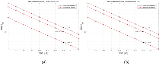
Figure 4. RMSE when the target and noise source are located on-axis (high SNR). (a) RMSE of ${\widehat{\theta }}_{\mathrm{azi}}$. (b) RMSE of ${\widehat{\theta }}_{\mathrm{ele}}$.

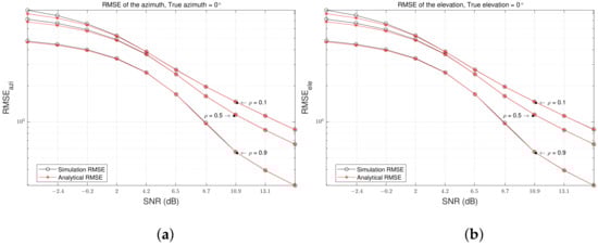
Figure 5. RMSE when the target and noise source are located on-axis (low SNR). (a) RMSE of ${\widehat{\theta }}_{\mathrm{azi}}$. (b) RMSE of ${\widehat{\theta }}_{\mathrm{ele}}$.

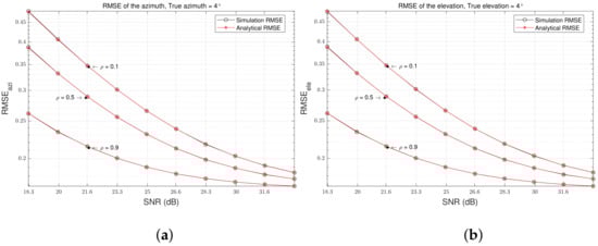
Figure 6. RMSE when the target’s azimuth and elevation are $4^{\circ }$. (a) RMSE of ${\widehat{\theta }}_{\mathrm{azi}}$. (b) RMSE of ${\widehat{\theta }}_{\mathrm{ele}}$.

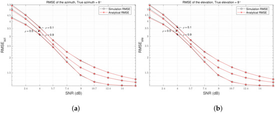
Figure 7. RMSE when the target’s azimuth and elevation are $8^{\circ }$. (a) RMSE of ${\widehat{\theta }}_{\mathrm{azi}}$. (b) RMSE of ${\widehat{\theta }}_{\mathrm{ele}}$.

Figure 4 and Figure 5 illustrate the dependence of the RMSE on the SNR and correlation coefficient with the increase in the SNR and correlation coefficient when the noise source and target are on the boresight axis (i.e., on-axis). In this case, it is assumed that the variances of the received noise variables are all equal. Figure 4 shows the RMSE results for a high SNR, and Figure 5 shows the RMSe results for a low SNR.

For a low SNR, many outliers occur at the estimated angle. Therefore, in Figure 5, when calculating the RMSE, outliers such as very large estimated angle values were filtered by limiting the upper and lower limits.

In Figure 4 and Figure 5, the results with the legend ‘Analytical RMSE’ show good agreements with those with the legend ‘Simulation RMSE’. Note that the RMSE decreases when the correlation coefficient increases from 0.1 to 0.9. That is, as the correlation between the received noise variables increases, the accuracy of the estimated angle increases.

In Table 1, the reduction rate of the RMSE for the increase in the correlation coefficient shown in Figure 4 is tabulated. The reduction rate of the RMSE for several correlation coefficients is calculated based on the RMSE result with a correlation coefficient of zero. For a high SNR and on-axis, the RMSE decreases by approximately 20% as the correlation coefficient between the received noise variables increases by 0.2.

Table 1. Reduction rate of RMSE with increasing correlation coefficient between noise variables at high SNR and on-axis.

	Correlation Coefficient between Noise Variables ($\mathit{\rho }$)
	0	0.2	0.4	0.6	0.8
Reduction rate of RMSE [%]	0	20.04	39.90	59.92	79.93

Figure 6 and Figure 7 illustrate the dependence of the RMSE on the increase in the SNR and correlation coefficient when the target and noise source are off-axis. In this case, the variances of the received noise variables are given differently. If the target and the noise source are closest to the A-beam as the angle of incidence increases, the noise variable with the largest variance is received from the A-antenna element, and the variances of the noise variables received from the remaining antenna elements are smaller than the variance of the noise variable received from the A-antenna element. In addition, because the C-antenna element is the furthest from the A-antenna element, the variance of the noise variable received from the C-antenna element is set to be the smallest. In Figure 6, the angles of incidence of the target are $4^{\circ }$, and in Figure 7, the angles of incidence of the target are $8^{\circ }$.

In Figure 6 and Figure 7, the results with the legend ’Analytical RMSE’ show good agreements with those with the legend ’Simulation RMSE’. Moreover, as the correlation coefficient increases from 0.1 to 0.9, the RMSE decreases. Consequently, the analytically derived RMSE is verified by confirming the same results in various cases via Figure 4, Figure 5, Figure 6 and Figure 7.

The dependence of the channel noise correlation coefficient on the ratio of the variances of the received noise variables is illustrated in Figure 8. The channel noise correlation coefficients (${\rho }_{azi,sum}$, ${\rho }_{ele,sum}$) defined in (21) and (22) are determined according to (19) and (20), which are the covariances of the channel noise. If we rearrange the expression in (19), we obtain

$$\begin{array}{c}\mathrm{cov}\left[n_{\mathrm{azi}},n_{\mathrm{sum}}\right]\hfill \\ ={\sigma }_{\mathrm{A}}^2+{\sigma }_{\mathrm{D}}^2-{\sigma }_{\mathrm{B}}^2-{\sigma }_{\mathrm{C}}^2+2{\rho }_{\mathrm{AD}}{\sigma }_{\mathrm{A}}{\sigma }_{\mathrm{D}}-2{\rho }_{\mathrm{BC}}{\sigma }_{\mathrm{B}}{\sigma }_{\mathrm{C}}\hfill \\ =\mathrm{E}\left[{\left(n_{\mathrm{A}}+n_{\mathrm{D}}\right)}^2\right]-\mathrm{E}\left[{\left(n_{\mathrm{B}}+n_{\mathrm{C}}\right)}^2\right].\hfill \end{array}$$

(42)

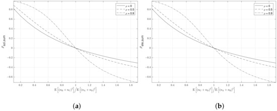
Figure 8. Channel noise correlation coefficient for noise variance ratio. (a) ${\rho }_{\mathrm{azi},\mathrm{sum}}$. (b) ${\rho }_{\mathrm{ele},\mathrm{sum}}$.

Here, $\mathrm{cov}\left[n_{\mathrm{azi}},n_{\mathrm{sum}}\right]$ consists of terms $\mathrm{E}\left[{\left(n_{\mathrm{A}}+n_{\mathrm{D}}\right)}^2\right]$ and $\mathrm{E}\left[{\left(n_{\mathrm{B}}+n_{\mathrm{C}}\right)}^2\right]$. $\mathrm{E}\left[{\left(n_{\mathrm{A}}+n_{\mathrm{D}}\right)}^2\right]$ is the variance of $n_{\mathrm{A}}+n_{\mathrm{D}}$ and $\mathrm{E}\left[{\left(n_{\mathrm{B}}+n_{\mathrm{C}}\right)}^2\right]$ is the variance of $n_{\mathrm{B}}+n_{\mathrm{C}}$. Therefore, Figure 8a illustrates the change of ${\rho }_{\mathrm{azi},\mathrm{sum}}$ with respect to the ratio of these two terms. Similarly, in Figure 8b, the change of ${\rho }_{\mathrm{ele},\mathrm{sum}}$ is illustrated with respect to the ratio of $\mathrm{E}\left[{\left(n_{\mathrm{C}}+n_{\mathrm{D}}\right)}^2\right]$ and $\mathrm{E}\left[{\left(n_{\mathrm{A}}+n_{\mathrm{B}}\right)}^2\right]$.

In Figure 8, as $\mathrm{E}\left[{\left(n_{\mathrm{B}}+n_{\mathrm{C}}\right)}^2\right]/\phantom{\mathrm{E}\left[{\left(n_{\mathrm{B}}+n_{\mathrm{C}}\right)}^2\right]\mathrm{E}\left[{\left(n_{\mathrm{A}}+n_{\mathrm{D}}\right)}^2\right]}\mathrm{E}\left[{\left(n_{\mathrm{A}}+n_{\mathrm{D}}\right)}^2\right]$ and $\mathrm{E}\left[{\left(n_{\mathrm{C}}+n_{\mathrm{D}}\right)}^2\right]/\phantom{\mathrm{E}\left[{\left(n_{\mathrm{C}}+n_{\mathrm{D}}\right)}^2\right]\mathrm{E}\left[{\left(n_{\mathrm{A}}+n_{\mathrm{B}}\right)}^2\right]}\mathrm{E}\left[{\left(n_{\mathrm{A}}+n_{\mathrm{B}}\right)}^2\right]$ increase, ${\rho }_{\mathrm{azi},\mathrm{sum}}$ and ${\rho }_{\mathrm{ele},\mathrm{sum}}$ gradually decrease to negative numbers. In addition, as the correlation coefficient of the received noise variables increases from 0 to 0.99, the average rate of change and the absolute value of the channel noise correlation coefficient increases.

Figure 9 illustrates the difference channel SNR result for the sum channel SNR. As the correlation coefficient of the received noise variable increases, the difference channel SNR becomes larger than the sum channel SNR. In the result of the legend of ‘$\rho =0$’, if the correlation coefficient is zero, the covariance terms in (16)–(18) are all canceled, so that the variance of the difference channel noise and the variance of the sum channel noise are equal (the SNR becomes the same). When the correlation coefficient increases to 0.99, the difference channel SNR increases than the sum channel SNR due to the covariance terms.

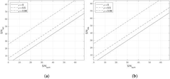
Figure 9. Difference channel SNR for sum channel SNR. (a) ${\mathrm{S}/\mathrm{N}}_{\mathrm{azi}}$ for ${\mathrm{S}/\mathrm{N}}_{\mathrm{sum}}$. (b) ${\mathrm{S}/\mathrm{N}}_{\mathrm{ele}}$ for ${\mathrm{S}/\mathrm{N}}_{\mathrm{sum}}$.

Figure 10, Figure 11, Figure 12, Figure 13, Figure 14 and Figure 15 illustrate how the RMSE is dependent on the channel noise correlation coefficient, difference channel SNR, and sum channel SNR. The x-axis is the difference channel SNR, and the y-axis is the sum channel SNR. The figures show the channel noise correlation coefficients of $-0.9$, 0, and $0.9$, respectively. In Figure 10, Figure 11 and Figure 12, the target’s azimuth and elevation errors are positive, and in Figure 13, Figure 14 and Figure 15, the target’s azimuth and elevation errors are negative. The RMSE is the lowest when the difference channel SNR and the sum channel SNR are 50dB, and the RMSE generally increases as the SNRs decrease. Overall, the RMSE increases more predominantly when the difference channel SNR decreases to 10 dB than when the sum channel SNR decreases to 10 dB. In Figure 10, Figure 11 and Figure 12, when the channel noise correlation coefficient increases from $-0.9$ to $0.9$, the RMSE decreases, whereas in Figure 13, Figure 14 and Figure 15, when the channel noise correlation coefficient increases from $-0.9$ to $0.9$, the RMSE rather increases.

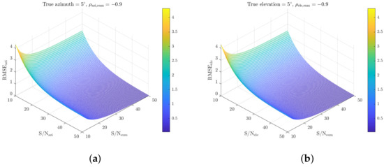
Figure 10. RMSE for difference channel SNR and sum channel SNR (${\theta }_{\mathrm{azi}},{\theta }_{\mathrm{ele}}=5^{\circ }$, ${\rho }_{\mathrm{azi},\mathrm{sum}}=-0.9$). (a) RMSE of ${\widehat{\theta }}_{\mathrm{azi}}$. (b) RMSE of ${\widehat{\theta }}_{\mathrm{ele}}$.

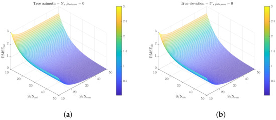
Figure 11. RMSE for difference channel SNR and sum channel SNR (${\theta }_{\mathrm{azi}},{\theta }_{\mathrm{ele}}=5^{\circ }$, ${\rho }_{\mathrm{azi},\mathrm{sum}}=0$). (a) RMSE of ${\widehat{\theta }}_{\mathrm{azi}}$. (b) RMSE of ${\widehat{\theta }}_{\mathrm{ele}}$.

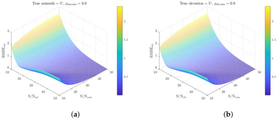
Figure 12. RMSE for difference channel SNR and sum channel SNR (${\theta }_{\mathrm{azi}},{\theta }_{\mathrm{ele}}=5^{\circ }$, ${\rho }_{\mathrm{azi},\mathrm{sum}}=0.9$). (a) RMSE of ${\widehat{\theta }}_{\mathrm{azi}}$. (b) RMSE of ${\widehat{\theta }}_{\mathrm{ele}}$.

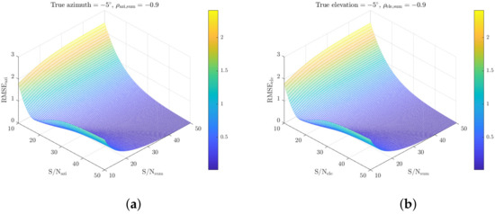
Figure 13. RMSE for difference channel SNR and sum channel SNR (${\theta }_{\mathrm{azi}},{\theta }_{\mathrm{ele}}=-5^{\circ }$, ${\rho }_{\mathrm{azi},\mathrm{sum}}=-0.9$). (a) RMSE of ${\widehat{\theta }}_{\mathrm{azi}}$. (b) RMSE of ${\widehat{\theta }}_{\mathrm{ele}}$.

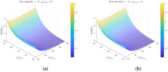
Figure 14. RMSE for difference channel SNR and sum channel SNR (${\theta }_{\mathrm{azi}},{\theta }_{\mathrm{ele}}=-5^{\circ }$, ${\rho }_{\mathrm{azi},\mathrm{sum}}=0$). (a) RMSE of ${\widehat{\theta }}_{\mathrm{azi}}$. (b) RMSE of ${\widehat{\theta }}_{\mathrm{ele}}$.

Figure 15. RMSE for difference channel SNR and sum channel SNR (${\theta }_{\mathrm{azi}},{\theta }_{\mathrm{ele}}=-5^{\circ }$, ${\rho }_{\mathrm{azi},\mathrm{sum}}=0.9$). (a) RMSE of ${\widehat{\theta }}_{\mathrm{azi}}$. (b) RMSE of ${\widehat{\theta }}_{\mathrm{ele}}$.

4. Comparison with Existing Performance Analysis Method

In this section, the analytic MSE expressions of the ACM algorithm from [14] are presented, and the results of the RMSE obtained via the analytic MSE expression of [14] and the numerical integration-based analytical RMSE presented in this paper are compared. The analytic MSEs are obtained using the Taylor series. These methods applied the second-order Taylor approximation to the original monopulse estimation equation, using the independent principle and moments of random variables in the process of deriving the MSEs of the estimation equations to which the Taylor approximation is applied. The analytic MSEs based on the second-order Taylor approximation proposed in the previous study are as follows [14]:

$$\begin{array}{c}\mathrm{E}\left[{\left({\widehat{\theta }}_{\mathrm{azi}}^{\prime }-{\theta }_{\mathrm{azi}}\right)}^2\right]\hfill \\ ={\sigma }_{\mathrm{A}}^2{\alpha }_{\mathrm{A}}^2+{\sigma }_{\mathrm{B}}^2{\alpha }_{\mathrm{B}}^2+{\sigma }_{\mathrm{C}}^2{\alpha }_{\mathrm{C}}^2+{\sigma }_{\mathrm{D}}^2{\alpha }_{\mathrm{D}}^2\hfill \\ +{\sigma }_{\mathrm{A}}^2{\sigma }_{\mathrm{B}}^2\left({\beta }_{\mathrm{AB}}^2+\frac{1}{2}{\beta }_{\mathrm{AA}}{\beta }_{\mathrm{BB}}\right)+{\sigma }_{\mathrm{A}}^2{\sigma }_{\mathrm{C}}^2\left({\beta }_{\mathrm{AC}}^2+\frac{1}{2}{\beta }_{\mathrm{AA}}{\beta }_{\mathrm{CC}}\right)\hfill \\ +{\sigma }_{\mathrm{A}}^2{\sigma }_{\mathrm{D}}^2\left({\beta }_{\mathrm{AD}}^2+\frac{1}{2}{\beta }_{\mathrm{AA}}{\beta }_{\mathrm{DD}}\right)+{\sigma }_{\mathrm{B}}^2{\sigma }_{\mathrm{C}}^2\left({\beta }_{\mathrm{BC}}^2+\frac{1}{2}{\beta }_{\mathrm{BB}}{\beta }_{\mathrm{CC}}\right)\hfill \\ +{\sigma }_{\mathrm{B}}^2{\sigma }_{\mathrm{D}}^2\left({\beta }_{\mathrm{BD}}^2+\frac{1}{2}{\beta }_{\mathrm{BB}}{\beta }_{\mathrm{DD}}\right)+{\sigma }_{\mathrm{C}}^2{\sigma }_{\mathrm{D}}^2\left({\beta }_{\mathrm{CD}}^2+\frac{1}{2}{\beta }_{\mathrm{CC}}{\beta }_{\mathrm{DD}}\right)\hfill \\ +{\sigma }_{\mathrm{A}}^4\left(\frac{3}{4}{\beta }_{\mathrm{AA}}^2\right)+{\sigma }_{\mathrm{B}}^4\left(\frac{3}{4}{\beta }_{\mathrm{BB}}^2\right)+{\sigma }_{\mathrm{C}}^4\left(\frac{3}{4}{\beta }_{\mathrm{CC}}^2\right)+{\sigma }_{\mathrm{D}}^4\left(\frac{3}{4}{\beta }_{\mathrm{DD}}^2\right),\hfill \end{array}$$

(43)

$$\begin{array}{c}E\left[{\left({\widehat{\theta }}_{\mathrm{ele}}^{\prime }-{\theta }_{\mathrm{ele}}\right)}^2\right]\hfill \\ ={\sigma }_{\mathrm{A}}^2{\alpha }_{\mathrm{A}}^2+{\sigma }_{\mathrm{D}}^2{\alpha }_{\mathrm{B}}^2+{\sigma }_{\mathrm{C}}^2{\alpha }_{\mathrm{C}}^2+{\sigma }_{\mathrm{B}}^2{\alpha }_{\mathrm{D}}^2\hfill \\ +{\sigma }_{\mathrm{A}}^2{\sigma }_{\mathrm{D}}^2\left({\beta }_{\mathrm{AB}}^2+\frac{1}{2}{\beta }_{\mathrm{AA}}{\beta }_{\mathrm{BB}}\right)+{\sigma }_{\mathrm{A}}^2{\sigma }_{\mathrm{C}}^2\left({\beta }_{\mathrm{AC}}^2+\frac{1}{2}{\beta }_{\mathrm{AA}}{\beta }_{\mathrm{CC}}\right)\hfill \\ +{\sigma }_{\mathrm{A}}^2{\sigma }_{\mathrm{B}}^2\left({\beta }_{\mathrm{AD}}^2+\frac{1}{2}{\beta }_{\mathrm{AA}}{\beta }_{\mathrm{DD}}\right)+{\sigma }_{\mathrm{D}}^2{\sigma }_{\mathrm{C}}^2\left({\beta }_{\mathrm{BC}}^2+\frac{1}{2}{\beta }_{\mathrm{BB}}{\beta }_{\mathrm{CC}}\right)\hfill \\ +{\sigma }_{\mathrm{B}}^2{\sigma }_{\mathrm{D}}^2\left({\beta }_{\mathrm{BD}}^2+\frac{1}{2}{\beta }_{\mathrm{BB}}{\beta }_{\mathrm{DD}}\right)+{\sigma }_{\mathrm{C}}^2{\sigma }_{\mathrm{B}}^2\left({\beta }_{\mathrm{CD}}^2+\frac{1}{2}{\beta }_{\mathrm{CC}}{\beta }_{\mathrm{DD}}\right)\hfill \\ +{\sigma }_{\mathrm{A}}^4\left(\frac{3}{4}{\beta }_{\mathrm{AA}}^2\right)+{\sigma }_{\mathrm{D}}^4\left(\frac{3}{4}{\beta }_{\mathrm{BB}}^2\right)+{\sigma }_{\mathrm{C}}^4\left(\frac{3}{4}{\beta }_{\mathrm{CC}}^2\right)+{\sigma }_{\mathrm{B}}^4\left(\frac{3}{4}{\beta }_{\mathrm{DD}}^2\right),\hfill \end{array}$$

(44)

where $\alpha$ and $\beta$ in (43) and (44) denote a first-order Taylor and a second-order Taylor coefficient, respectively. For the detailed derivation of Equations (43) and (44), refer to [14]. The above equations are derived by assuming that the received noise variables are all uncorrelated. Therefore, in order to compare with the method proposed in this paper, all correlation coefficients are set to zero.

Figure 16 shows the results of the numerical integration-based analytical RMSE proposed in this paper and the second-order Taylor approximation-based RMSE proposed in [14]. The results of the integration-based MSE completely overlap the simulation-based MSE results. On the other hand, the results of the second-order Taylor approximation based-analytic MSE show quite large differences from the above results of two MSE methods. The reason for these differences is that the analytic MSE equations are derived by applying several approximations, so there are differences between the simulation-based MSE using the original monopulse estimation equation and the analytic MSE. Moreover, this Taylor approximation-based analytical expression is valid only when the correlation coefficient is zero.

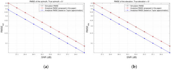
Figure 16. Comparison of RMSE results using analytic expression based on Taylor approximation and analytic expression based on numerical integration. (a) RMSE of ${\widehat{\theta }}_{\mathrm{azi}}$. (b) RMSE of ${\widehat{\theta }}_{\mathrm{ele}}$.

5. Discussion

In Section 3, first, the analytical RMSE is verified by comparing the results of the Monte Carlo simulation-based RMSE for various cases. In Figure 4, Figure 5, Figure 6 and Figure 7, it can be seen that the analytical RMSE result and the Monte Carlo simulation RMSE result show excellent agreements for the case where the SNRs are different and several correlation coefficients of the received noise variables are given. The RMSE results are consistent, but the operation times are not. The analytical RMSE calculates the main occurrence region of the noise variables through the PDF. In this respect, it can be calculated more efficiently and accurately than the Monte Carlo-based MSE, which is dependent on the number of repetitions.

In Figure 4, Figure 5, Figure 6 and Figure 7, it is confirmed that the RMSE decreased as the correlation coefficient between the received noise variables approached one. The reason why these results occur is that when the correlation coefficient approaches one, the correlated noises in the difference channel cancel each other out, so the SNR of the difference channel increases.

In Figure 8a, the fact that $\mathrm{E}\left[{\left(n_{\mathrm{B}}+n_{\mathrm{C}}\right)}^2\right]/\phantom{\mathrm{E}\left[{\left(n_{\mathrm{B}}+n_{\mathrm{C}}\right)}^2\right]\mathrm{E}\left[{\left(n_{\mathrm{A}}+n_{\mathrm{D}}\right)}^2\right]}\mathrm{E}\left[{\left(n_{\mathrm{A}}+n_{\mathrm{D}}\right)}^2\right]$ is less than 1 denotes that the magnitude of the noise received by the antenna elements B and C is larger than the magnitude of the noise received by the antenna elements A and D. Moreover, it can be explained that the noise source is located in the positive azimuth direction with respect to the boresight. Conversely, if $\mathrm{E}\left[{\left(n_{\mathrm{B}}+n_{\mathrm{C}}\right)}^2\right]/\phantom{\mathrm{E}\left[{\left(n_{\mathrm{B}}+n_{\mathrm{C}}\right)}^2\right]\mathrm{E}\left[{\left(n_{\mathrm{A}}+n_{\mathrm{D}}\right)}^2\right]}\mathrm{E}\left[{\left(n_{\mathrm{A}}+n_{\mathrm{D}}\right)}^2\right]$ is greater than 1, it can be said that the noise source is located in the negative azimuth direction with respect to the boresight. This is explained equally for elevation.

In Figure 8, when the power of the received noise dominates in the positive direction in the azimuth and elevation, the correlation coefficient of the channel noise is positive, and when the power of the received noise dominates in the negative direction, the correlation coefficient of the channel noise is negative. Moreover, when the correlation coefficient between the received noise variables increases, the change in the channel noise correlation coefficient becomes larger as the ratio of the received noise variances is changed, and the absolute value of the channel noise correlation coefficient is larger.

In summary, it can be explained that if the correlation coefficient between the received noise variables increases, the absolute value of the correlation coefficient of the channel noise increases and the RMSE of the estimated angle decreases. This is consistent with the results shown in [16]. Reference [16] explains that the larger the correlation coefficient between channels, the narrower the MR deviation becomes. The narrower the deviation of the MR, the more precise the estimated angle.

Figure 10, Figure 11 and Figure 12 show the result that the RMSE decreases as the correlation coefficient of the channel noise increases from negative to positive when the target’s azimuth and elevation are positive. On the other hand, in Figure 13, Figure 14 and Figure 15, when the azimuth and elevation of the target are negative, the RMSE decreases as the correlation coefficient of the channel noise decreases from positive to negative. In Figure 8, we find that the correlation coefficient of the channel noise changes from negative to positive when the noise source changes from negative to positive in the azimuth and elevation directions with respect to the boresight. Consequently, referring to the results of Figure 8 and Figure 10, Figure 11, Figure 12, Figure 13, Figure 14 and Figure 15, when the noise source and the target have the same sign in the azimuth and elevation directions, the RMSE decreases, and when the sign is different, the RMSE increases.

6. Conclusions

In general, ACM radar uses four squinted beams to simultaneously estimate azimuth and elevation. When noise from an external source is present, the noise is received in the four squinted beams, and the accuracy of estimating the angle of the target by the radar becomes low. Assuming this environment, in this study, we analyzed the RMSE of the ACM algorithm with an analytical equation in various cases by varying the correlation and variance of the noise variables received by the four antenna elements.

For verification, the results of the Monte Carlo simulation-based RMSE and the analytic equation-based RMSE are compared by varying the SNR and angle of incidence. It is confirmed that the results of the analytically derived RMSE equation and the Monte Carlo-based simulation RMSE are in good agreement. Moreover, we find that the absolute value of the channel noise correlation coefficient increases and the RMSE of the estimated angle decreases when the correlation coefficient between the received noise variables increases. In particular, when the SNR is high and the noise source is located on the axis, the RMSE decreases by 20% whenever the correlation coefficient between the reception noise variables increases by 0.2.

Referring to the results of the RMSE for the difference channel SNR and sum channel SNR and the results of the channel noise correlation coefficient for the noise variance ratio, it is confirmed that the RMSE decreases when the signs of the direction of the noise source and the target are the same, and the RMSE increases when the signs are different. Here, the same sign denotes that the azimuth or elevation direction of the target and the noise source with respect to the boresight is the same.

In this paper, it is assumed that the correlation coefficients between the received noise variables are all the same. However, in general, the correlation coefficients are different. In a future study, we will derive a correlation coefficient expression that depends on the direction of the noise signal, such as noise jamming, and will explicitly analyze the RMSE performance for the direction of the noise signal.

References

- Sherman, S.M.; Barton, D.K. Monopulse Principles and Techniques; Artech House: Norfolk County, MA, USA, 1984. [Google Scholar]
- Rhodes, D.R. Introduction to Monopulse; Artech House: Norfolk County, MA, USA, 1980. [Google Scholar]
- Leonov, A.I.; Fomichev, K.I. Monopulse Radar; Artech House: Norfolk County, MA, USA, 1986. [Google Scholar]
- Park, S.R.; Nam, I.K.; Noh, S.U. Modeling and simulation for the investigation of radar responses to electronic attacks in electronic warfare environments. Secur. Commun. Netw. 2018, 2018, 3580536. [Google Scholar] [CrossRef]
- Bassem, R.M. Radar Systems Analysis and Design Using MATLAB, 3rd ed.; CRC Press: Boca Raton, FL, USA, 2013. [Google Scholar]
- Eaves, J.L.; Reedy, E.K. Principles of Modern Radar; Chapman and Hall: New York, NY, USA, 1987. [Google Scholar]
- Wang, Z.; Zeng, Y.; Liu, M.; Yang, Q. Investigation of the related factors of angle measurements precision in monopulse radar. In Proceedings of the 2017 International Applied Computational Electromagnetics Society Symposium (ACES), Firenze, Italy, 26–30 March 2017; pp. 1–2. [Google Scholar]
- Jacovitti, G. Performance analysis of monopulse receivers for secondary surveillance radar. IEEE Trans. Aerosp. Electron. Syst. 1983, AES-19, 884–897. [Google Scholar] [CrossRef]
- Kim, M.J.; Hong, D.S.; Park, S.S. A study on the amplitude comparison monopulse algorithm. Appl. Sci. 2020, 10, 3966. [Google Scholar] [CrossRef]
- Chen, L.; Sheng, W. Performance analysis for angle measurement of monopulse radar with non-consistent amplitude-phase features. In Proceedings of the IEEE 2010 International Conference on Microwave and Millimeter Wave Technology, Chengdu, China, 8–11 May 2010. [Google Scholar]
- Yu, K.-B.; Murrow, D.J. Adaptive digital beamforming for preserving monopulse target angle estimation accuracy in jamming. In Proceedings of the 2000 IEEE Sensor Array and Multichannel Signal Processing Workshop, Cambridge, MA, USA, 16–17 March 2000; pp. 454–458. [Google Scholar]
- Zhang, X.; Li, Y.; Yang, X.; Zheng, L.; Long, T.; Baker, C.J. A novel monopulse technique for adaptive phased array radar. Sensors 2017, 17, 116. [Google Scholar] [CrossRef] [PubMed] [Green Version]
- Dong, W.; Wang, J.; Song, Z. Mono-pulse radar angle estimation algorithm under low signal-to-noise ratio. J. Phys. Conf. Ser. 2021, 1914, 012042. [Google Scholar] [CrossRef]
- An, D.J.; Lee, J.H. Performance analysis of amplitude comparison monopulse direction-of-arrival estimation. Appl. Sci. 2020, 10, 1246. [Google Scholar] [CrossRef] [Green Version]
- Ham, H.W.; Lee, J.H. Improvement of performance analysis of amplitude-comparison monopulse algorithm in the presence of an additive noise. Electronics 2021, 10, 2649. [Google Scholar] [CrossRef]
- Kanter, I. The ratios of functions of random variables. IEEE Trans. Aerosp. Electron. Syst. 1977, AES-13, 624–630. [Google Scholar] [CrossRef]
- Groves, G.W.; Blair, W.D.; Chow, W.C. Probability distribution of complex monopulse ratio with arbitrary correlation between channels. IEEE Trans. Aerosp. Electron. Syst. 1997, 33, 1345–1350. [Google Scholar] [CrossRef]
- Seifer, A.D. Monopulse-radar angle measurement in noise. IEEE Trans. Aerosp. Electron. Syst. 1994, 30, 950–957. [Google Scholar] [CrossRef]
- Yuan, C.; Weihua, F.; Lin, L.; Keyu, T.; Jin, Y. A quantitive method to assess monopulse radar seeker angle measurement performance in the presence of noise jamming. In Proceedings of the 2011 IEEE CIE International Conference on Radar, Chengdu, China, 24–27 October 2011. [Google Scholar]
- Richards, M.A.; Scheer, J.A.; Holm, W.A. Principles of Modern Radar Basic Principles; SciTech Publishing Inc.: Raleigh, NC, USA, 2008; Volume 1. [Google Scholar]
- Yates, R.D.; Goodman, D.J. Probability and Stochastic Processes, 3rd ed.; John Wiley and Sons: Hoboken, NJ, USA, 2014. [Google Scholar]
- Guo, Y.F.; Yin, Z. Exact Distributions of the Sum of Two Standard Bivariate Normal Dependent Random Variables. In Proceedings of the 2010 4th International Conference on Bioinformatics and Biomedical Engineering, Chengdu, China, 18–20 June 2010; pp. 1–5. [Google Scholar] [CrossRef]
Publisher’s Note: MDPI stays neutral with regard to jurisdictional claims in published maps and institutional affiliations. |
© 2022 by the authors. Licensee MDPI, Basel, Switzerland. This article is an open access article distributed under the terms and conditions of the Creative Commons Attribution (CC BY) license (https://creativecommons.org/licenses/by/4.0/).