An Adaptive Threshold Line Segment Feature Extraction Algorithm for Laser Radar Scanning Environments

Abstract

An accurate map is needed for the autonomous navigation of mobile robots in unknown environments. The application of laser radars has the advantages of high ranging accuracy and long ranging distances. Due to the small amount of data on laser radars and the influence of noise on the sensor itself, these amount to causing problems such as low accuracies of map construction and large positioning errors. Currently, the feature extraction of environmental line segments based on radar scanning data generally adopts the idea of recursion. However, the amount of calculations for applying recursion is large, and the threshold of extracted feature points needs to be set manually. Moreover, the fixed segmentation threshold will cause under-segmentation or over-segmentation. In this paper, an adaptive threshold-based feature extraction method for environmental line segments is proposed. The method denoises the original data first, and then an adaptive threshold of the nearest neighbor algorithm is provided to improve the accuracy of breakpoint judgment; next, the slope difference between adjacent line segments is evaluated according to the line segment fitting error in order to obtain the optimal corner feature. Finally, the point set is segmented to fit line-segment features. Based on actual environment tests, the environmental similarity of the line segment features extracted by the new algorithm in this paper increases by 8.3% compared with the IEPF (Iterative End Point Fit) algorithm. The algorithm avoids recursive operations, improves the efficiency by four times, and meets the real-time requirements of line segment fitting.

1. Introduction

Two-dimensional radars are widely used in daily mobile robots, with advantages of high ranging accuracy, little influence of ambient illumination on equipment, and so on. The disadvantage is that the amount of data obtained from one frame of radar scanning information is small, and the environmental feature information that can be extracted is limited [1]. Therefore, it is particularly important to process the raw data of each frame of 2D Radar and extract line segment features; In particular, in weak texture environments, environmental features are degraded. Processing the point feature of the environment to form line features [2] can improve navigation accuracy and robustness effectively, which is a key for mobile robots to locate and navigate independently in complex environments [3]. In addition, the perfect map information can clarify the location of mobile robot in the environment, which serves for path planning [4] and improves work efficiency. Map information is usually composed of geometric primitives processed by environmental feature points, including geometric configurations such as arcs, line segments, and right angles. If these features can be used, the positioning accuracy of the SLAM algorithm will be improved [5]. Among them, the line segment is the most common obstacle contour feature [6]. However, the change of observation position leads to the formation of breakpoints and the change of corner positions, and the effect is not good in practice. Therefore, the method of extracting line segment features [7] from 2D Lidar scanning data still needs to be further studied.

Currently, the extraction of line segment features is mainly composed of three parts: data pre-processing, breakpoint detection, and line extraction. In document [8], a framework for geometrical feature detection in 2D range images is proposed. It is found that, in every segmentation algorithm, robustness can only be expected up to a certain level of outliers. The adaptive breakpoint detector [9] determines the detection threshold by extrapolating the radius of the threshold circle under the most extreme acceptable condition, but the threshold error is large when the obstacle is particularly close to the origin or the obstacle plane coincides with the incident laser. The kalman filter (KF) breakpoint detector [10] tracks an approximate kinematic model from the observation data to verify whether the two continuous distance points belong to the same region, but it receives great limitations in the nonlinear scene, resulting in an incorrect judgment threshold. The line tracking (LT) [11] method judges whether the distance from the next point to the current line segment is less than the threshold, and the calculation speed of this process is very fast and universal, although it is difficult to determine a suitable threshold, especially in the case of unknown map size and error. If the threshold is inaccurate, it is very likely to divide the point that should belong to the next line segment into the current point set erroneously, and the line tracking method does not have a merging process [12]; iterative end-point fit (IEPF) [13] and split-and-merge (SM) [14] adopt recursive ideas, which comprise fast calculation speeds and good adaptability to local maps, but the judgment process also needs the point-to-point distance threshold and the point-to-line distance threshold. If the threshold is given inaccurately, it will also cause under-segmentation and over-segmentation. Therefore, it is sensitive to the given judgment threshold [15]. The prototype-based fuzzy clustering [16] method is sensitive to the initial prototype by continuously reducing the cost function for segment segmentation, and the number of prototypes must be a priori. Therefore, it is vulnerable to outliers in the process of fuzzy clustering. Other methods, such as the Hough transform [17], possess the advantages of simple geometric resolution and parallel extraction, but they require high discretizations of point clouds. The algorithm judges whether there is a straight line by the number of points on the straight line, which has a large amount of calculation and cannot guarantee the real-time feature extraction of line segments.

The above methods use a fixed threshold for judgenents and cannot obtain the optimal feature points for different radars or complex environments. Firstly, because the parameters of different 2D radars and the noise errors generated by the sensors are different [18], and the distribution of points scanned on obstacles with line segment features is uneven. Furthermore, the farther the radar scans, the greater the error of the collected data is. When detecting breakpoints and corner features, fixed thresholds cannot avoid the loss of segment features [19]. Therefore, this paper proposes an environmental line segment feature extraction algorithm based on adaptive threshold, which can avoid iterative calculation and reduce the amount of computation effectively. Moreover, it can solve the problem of difficult threshold selection in line segment feature extraction and improve the accuracy of line segment feature extraction.

The rest of this paper is organized as follows: Section 2 describes feature extraction algorithm of the line segment. After denoising radar data, an adaptive threshold algorithm is used to detect breakpoints and corners, and these data are segmented to fit into line segments; Section 3 describes the feature extraction algorithm steps of environmental line segment with adaptive threshold; the fourth section tests the feasibility of the algorithm in the actual environment and compares it with other algorithms; the fifth section summarizes the laser line segment feature extraction algorithm based on an adaptive threshold.

2. Line Segment Feature Extraction

2.1. Noise Reduction of Radar Data

The measurement accuracy of sensor is affected by the environment and device characteristics. The noise interference of laser radar will lead to some isolated points [20] in the data, but this is not the real observation data, which will affect the algorithm results and should be filtered in advance. Therefore, in order to reduce the influence of noise information on line segment feature extraction and improve mapping accuracy, it is necessary to denoise raw data from radar scanning [21]. In addition, when the laser radar collects remote environmental information, the collected data points are highly discrete [22], and the error will increase, resulting in uneven distribution of scanned points, and the fitting line segment is quite different from the real environment.

Figure 1 shows the ranging model of radar; the output is a series of measured distance information. Δθ represents the angle between two adjacent laser beams, namely the angular resolution of lidar, and the unit is rad; θ_i is the angle of the ith laser in the rectangular coordinate system, and the unit is rad; P_i is the laser scanning point i, and the unit is m. Based on the distribution of obstacles, there will be breakpoints, corners, and a small amount of noise. The break point refers to the edge point of the inconsistent obstacle contour, the corner point refers to the corner point of the obstacle contour that is the intersection of two lines, and noise point refers to the distorted data point affected by noise. Laser radar data are sorted from the start angle to the end angle in a counterclockwise fashion, and the form of laser radar point cloud can be obtained as $P=\{\left({\rho }_i,{\theta }_i\right)\mid i=1,2,\cdots ,N\}$, where (P_i, θ_i) is the polar coordinate of the first laser scanning point; ρ_i is the distance from the obstacle reflection point measured in the θ_i direction to the laser radar launch point; N is the number of laser points in a frame. In the scanning process of Lidar, there are two types of sensor errors: One is Gaussian white noise n_i in the measurement process. White noise is the noise with equal noise energy in a wide frequency range and the frequency band of each bandwidth, and its probability density function obeys Gaussian distributions [23,24]. One is the measurement error b_i of the sensor itself, which is a comprehensive parameter of the internal error of the sensor caused by various physical factors such as internal machinery, temperature, and so on. The system error is generally provided by the manufacturer. As a result, the relationship between laser radar measurement distance ρ_i and real obstacle distance ρ_v is described as follows.

$${\rho }_i={\rho }_v+b_i\left({\rho }_i\right)+n_i$$

(1)

In order to facilitate the search for noise points, polar coordinate data collected by each frame of radar are converted into a rectangular coordinate system. The measured distance is represented by x_i and y_i with respect to the rectangular coordinate system of the sensor. The solution method is described as follows.

$${\theta }_i=\left(\Delta \theta ·i-\alpha \right)·\frac{\pi }{180}$$

(2)

$$\{\begin{array}{c}{x}_i={\rho }_i cos {\theta }_i\\ y_i={\rho }_i sin {\theta }_i\end{array}$$

(3)

In the above formula, i is the laser beam i; θ_i is the angle of the laser beam i in the rectangular coordinate system; Δθ is the angular resolution of the radar; α is the starting angle of the radar measurement, and the unit is rad; ρ_i is the distance from the reflection point to the emission point measured by laser beam i.

The distance between two adjacent measurement points is denoted by d_i.

$$d_i=\sqrt{{\left(x_{i+1}-x_i\right)}^2+{\left(y_{i+1}-y_i\right)}^2}$$

(4)

In the above formula, i is the data point i in the point set; θ_i is the angle of the data point i.

In order to make the final fitting line segment characteristics close to the real environment, a filtering algorithm [25] was used for processing. Based on the fixed angle difference between laser radar data points, this paper uses the mean filtering method to make the data smoother. Mean filtering sets the data window size as N first and replaces the value of isolated feature points in the point set with the mean value of all points in its neighborhood. After replacement, the value of feature points is closer to the real value, which can reduce over-segmentation effectively. The calculation formula of mean filtering is as follows.

$$P_{ave}=ave\left\{P_i,P_{i+1},\cdots P_{i+N-1}\right\}$$

(5)

In the above formula, P_ave represents the mean of all points in the window; ave represents the calculation function of the mean; P_i represents the original data point set; N is the size of the data window set by the mean filter. Setting the mean filter window size and replacing the current noise point and the value of two adjacent points with the mean value P_ave of the window data volume, data preprocessing steps were completed. Figure 2 is the effect of noise reduction of the original data point set of laser radar. Figure 2a shows that the polar coordinate data collected by the lidar are converted to the rectangular coordinate system, and the measured distance is relative to the coordinates of the lidar on the x-axis and y-axis, with the unit of m. Black points are the raw data points collected. It can be seen that the distribution of black points on the line segment is uneven, which can easily cause false judgments of corner points. The red points are the preprocessed data points after noise reduction. It can be seen that the data points are smoother and more evenly distributed on the line segment. In Figure 2b, the blue curves are the distance between adjacent points of the raw point set. It can be seen that the distance between points affected by noise fluctuates greatly. The red curves represent the distance between adjacent points of the preprocessed data point set after noise reduction. It can be observed that the distance between points fluctuates less and is closer to the real environment. The results show that the algorithm can reduce the over-segmentation of the line segment. Some data points that deviate from the line segment are close to the real value of the environment, which improves the accuracy of subsequent breakpoints and corner extraction.

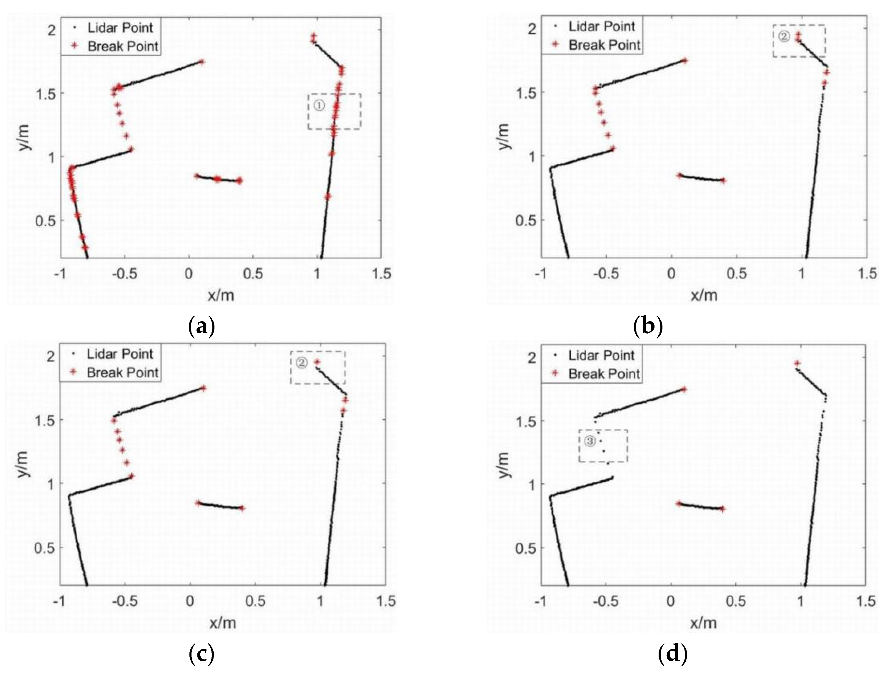
2.2. Breakpoint Detection of Adaptive Nearest Neighbor Algorithm

The principle of the nearest neighbor algorithm to detect breakpoints is that the points on the surface of the same object are continuous. In a frame of point cloud data, the same object surface will reflect back a continuous set of points, and the positions of these data points are adjacent. If the position between two adjacent points changes suddenly, it usually means that these two points come from two different object surfaces or sections. Therefore, whether the positions of two adjacent points are mutated can be used to judge whether the two points belong to the same class [26]. The more stable the position changes of two points, the more likely the two points belong to the same object.

Compare distance d_i between two adjacent measurement points with the breakpoint detection threshold D, and if d_i < D, the two adjacent measurement points are classified as the point set of the same obstacle. Conversely, for extract breakpoints i, point i is the end point of the previous straight line, point i + 1 is the starting point of the next straight line, and the point set of the original data is preliminarily divided. Traverse all the data points, judge according to this method, and divide the frame data into several point sets. The nearest neighbor algorithm detects breakpoints with simple calculation and fast processing speed. The detection process depends on the selection of the distance threshold D. The value of D not only affects the effect of the initial segmentation but also affects the accuracy and completeness of the subsequent line segment fitting. Figure 3 shows the characteristics of the laser point scanned by the lidar. Figure 3a shows that the polar coordinate data collected by the lidar is converted to the rectangular coordinate system, and the measured distance is relative to the coordinates of the lidar on the x-axis and y-axis with the unit of m. The scanning beam of the lidar is fan-shaped. Since the angular resolution of the same lidar is fixed, the angular resolution of the radar will decrease when the distance is far, which will make the laser point on the close obstacle more dense and the laser point on the long-distance obstacle relatively dispersed. Figure 3b shows the distance between the adjacent laser points in Figure 3a, that is, the 200th point to the 250th point in a frame, including the laser points of close obstacles and long-distance obstacles. It can be observed that as the distance between the adjacent two points increases, threshold D should also increases accordingly. Therefore, the traditional algorithm uses a fixed threshold [27], which cannot meet the feature extraction of complex scenes. Therefore, this paper first designs an adaptive threshold D selection method as follows.

Therefore, the selected breakpoint detection threshold D should be adaptively changed according to the distance measured by the laser, as shown in formula (6).

$$\Delta d_i=2 {\rho }_i sin \frac{\Delta \theta }{2}$$

(6)

In the above formula, Δd_i is the distance between two adjacent points and, the unit is m; ρ_i is the distance measured by the laser beam i; θ_i is the angular resolution of the radar. The angular resolution is the angle between two adjacent laser points. When the angle is too large, the laser points are dispersed, which may lead to a loss of key shape characteristics of the environment. Therefore, laser radar with small angular resolution should be selected. In order to meet the acquisition of indoor environmental characteristics, the angular resolution of laser radar used in this paper is 0.33°, and when Δθ is very small, sin Δθ ≈ Δθ.

$$D=k·\Delta d_i=k·{\rho }_i·\Delta \theta ·\pi /180$$

(7)

In the above formula, k is a fixed value that needs to be determined by the current radar. When distance ρ_i measured by the laser increases, distance Δd_i between two adjacent points also increases, and k is the amplification factor of the current breakpoint detection threshold. When the result of breakpoint detection is the same as the real environment, it is the most suitable k value, and the initial segmentation of the original point set is completed at this time. In order to determine the amplification factor k of the current radar, when k = 1, 3, 5, 10, several comparison experiments of breakpoint detection are performed, as shown in Figure 4.

It can be observed from Figure 4 that when the amplification factor k = 1, the distribution in region 1 is not uniform. The point that should have belonged to the same obstacle was mistakenly determined as a breakpoint, and the magnification factor was too small. When the magnification factor k = 3, the breakpoint segmentation results are consistent with the real environment. When the amplification coefficient k = 5, the breakpoint part in Region 2 is not extracted because the distance between adjacent points is smaller than the breakpoint detection threshold due to the existence of noise. When the magnification factor k = 10, the small obstacles in region 3 do not extract breakpoints but regard them as points on the same line segment, where the magnification factor is too large. According to the experimental results of this laser radar, when the amplification factor k = 3, the breakpoint detection effect is the best.

If the threshold is too small, the radar data belonging to the same object surface will be segmented into different points. Although judgment accuracy is high, segmentation is too cumbersome, which weakens the real-time performance of detection. On the contrary, if the threshold is too large, it is difficult for small obstacles to be detected, resulting in the missed detection of obstacles. In this paper, the data processing method based on the nearest distance clustering is selected, and the adaptive threshold is determined for the two-dimensional laser radar adapting to different distances so as to improve clustering accuracy and to realize obstacle detection under different distances.

2.3. Adaptive Threshold Segmentation

After completing the initial segmentation of the original point set, it is necessary to segment each part of the point set to find the corner features [28]. The original data distribution collected by the Lidar is shown in Figure 5. Point O is the laser emission point, the collected data points are P₁,P₂,P₃,P₄,⋯,P_n in that order, and the lengths from point O to the intersection point are ρ₁,ρ₂,ρ₃,ρ₄,⋯,ρ_n in that order; among them, point P₄ is the infinity point, so the value of ρ₄ is inf, P₃ and P₅ are breakpoints, and P₃ is the end point of the previous line. P₅ is the starting point of the next line, and P₇ is the corner feature to be extracted. Make a vertical line from point P_i to point OP_i+1 and intersect them at point P_i^′; φ_i is the angle between P_iP_i+1 and P_iP_i^′, where Δθ is the angular resolution of the Lidar.

On the line segment P₁P₃, the following derivation can be obtained based on the following geometric relationship.

$${\phi }_1={\phi }_2+\Delta \theta$$

(8)

$$tan {\phi }_1=\frac{P_1^{\prime }{P}_2}{P_1{P}_1^{\prime }}\approx \frac{{\rho }_1-{\rho }_1}{{\rho }_1·sin\Delta \theta }$$

(9)

On the line segment P₅P₇, the following derivation can be obtained based on the geometric relationship.

$${\phi }_6={\phi }_5+\Delta \theta$$

(10)

$$tan {\phi }_5=\frac{P_5^{\prime }{P}_6}{P_5{P}_5^{\prime }}\approx \frac{{\rho }_6-{\rho }_5}{{\rho }_5·sin\Delta \theta }$$

(11)

The default angular resolution of the Lidar used in this paper is 0.33°, and when Δθ is very small, sin Δθ ≈ Δθ. To reduce time cost of computation further, we use the following.

$$tan{\phi }_i\approx \frac{\mid {\rho }_{i+1}-{\rho }_i\mid }{{\rho }_i·\Delta \theta }$$

(12)

Among them, ρ_i is the distance measured by the laser beam i; ρ_i+1 is the distance measured by the laser beam i + 1. When the value of tan φ_i and tan φ_i+1 is less than the corner judgment threshold, point i and point i + 1 are considered points on the same line segment. When the value of tan φ_i and tan φ_i+1 is greater than the corner judgment threshold, it is considered that point i and point i + 1 are not on the same line segment.

The slope difference Δk(i) between two adjacent points is calculated as follows.

$$\Delta k\left(i\right)=\frac{\mid {\rho }_i-{\rho }_{i-1}\mid }{{\rho }_{i-1}·\Delta \theta }-\frac{\mid {\rho }_{i+1}-{\rho }_i\mid }{{\rho }_i·\Delta \theta }$$

(13)

In the formula, Δθ is the angular resolution of the Lidar, and when point P_i is the intersection of the straight line L1 and the straight line L2, then P_i is the corner point of the two straight lines. When ∣Δk(i)∣ > dk_th, ∣Δk(i)∣ > ∣Δk(i − 1)∣, and ∣Δk(i)∣ > ∣Δk(i + 1)∣, point i is the corner point, which is the end point of the previous straight line and the starting point of the next straight line. dk_th is the threshold for corner extraction, the disadvantage of the traditional fixed threshold is that it can easily cause over-segmentation or under-segmentation of the line segment feature extraction. In view of this, this paper proposes an adaptive threshold algorithm, which evaluates the effect of segmentation according to the fitting error of the line segment segmentation point set until the most suitable dk_th is found. In order for the average fitting error of all line segments to be minimized, and the segmentation point set is output. Figure 6a shows the calculated Δk(i) of 481 data points collected by laser radar. When the difference of Δk(i) values between two adjacent points is small, it is considered that the two points are in the same line; otherwise, the point is a breakpoint or an independent point, and the maximum value of Δk(i) in the figure is 0.052 m. Figure 6b is the enlarged graph from 356th point to 372th point in (a). In area 1, Δk(i) of point 364 has an obvious peak value, and the peaks of point 363 and point 365 are slightly smaller, satisfying ∣Δk(i)∣ > ∣Δk(i − 1)∣, and ∣Δk(i)∣ > ∣Δk(i + 1)∣. When ∣Δk(i)∣ > dk_th, it is a corner feature. When Δk(i) conforms to the corner feature and has a peak value; if ∣Δk(i) − Δk(i − 1)∣ < ∣Δk(i) − Δk(i + 1)∣, the corner should be between point i − 1 and point i. On the contrary, the corner should be between point i and point i + 1. When the range of the corner extraction threshold dk_th is selected (0, 0.052) and the number of evaluations is set to less than 100 times, then the threshold is increased by 0.01 each time.

The calculation formula of SSE (Sum of the Squared Errors) for line segment fitting errors is shown in (14).

$$SSE=\sum _{i=1}^n{W}_i\left(y_i-y_i^{\prime }\right)$$

(14)

In the formula, SSE is the sum of squares of errors corresponding to the predicted data and the original data, W_i indicates the weight, y_i is the original data, $y_i^{\prime }$ is the predicted data, and the unit is m.

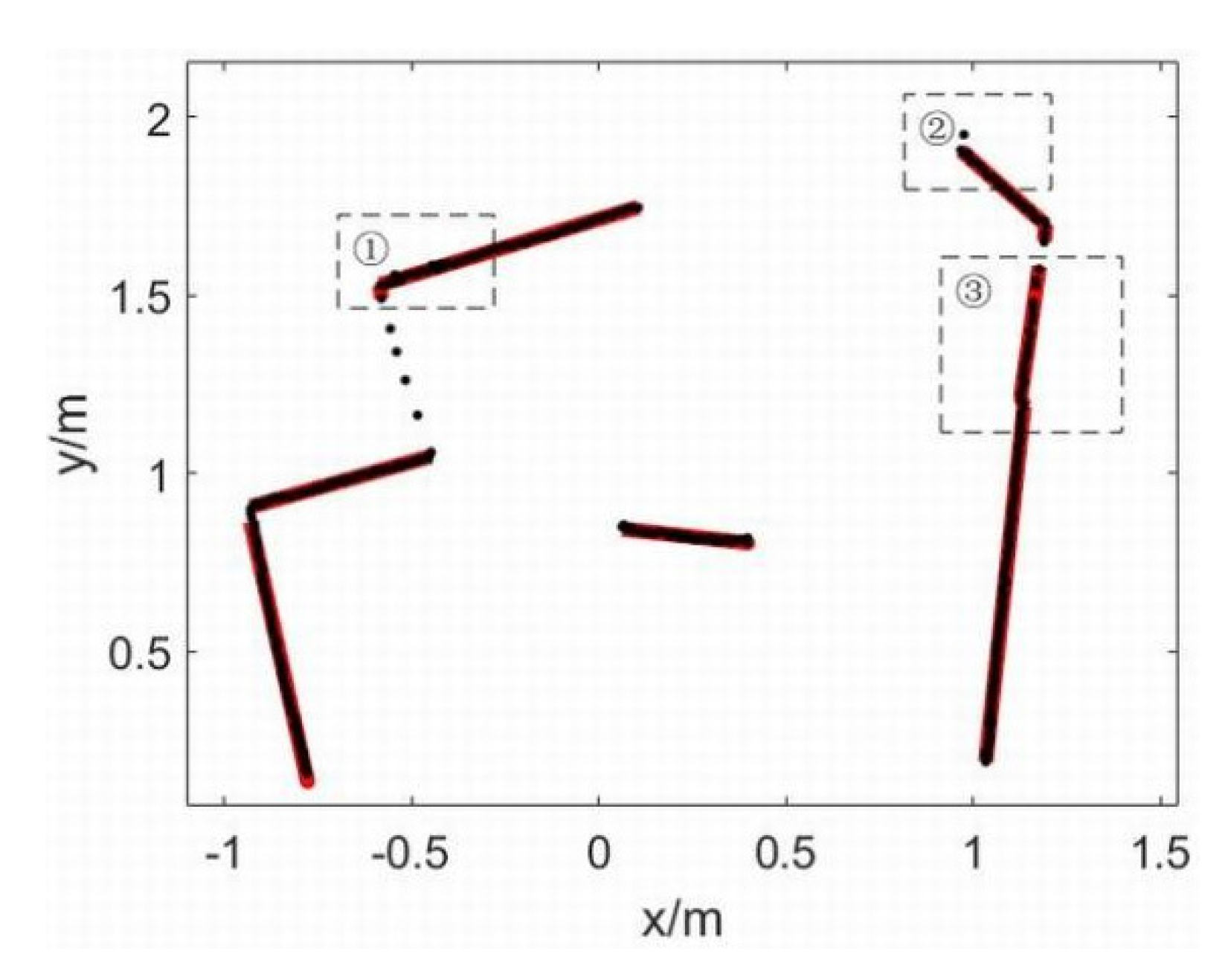
2.4. Piecewise Fitting of Point Set

When the Lidar scans the environment, it obtains discrete scanning points. There is a certain error between the position of corner feature extracted from the scanning points and the real physical corner position [29], especially when the physical corner is far away from the Lidar, the error will be large. In order to reduce the difference between the extracted corner feature positions and the real physical corner positions, it is necessary to precisely locate the possible corner points obtained after preliminary line segment segmentation [30]. The process of line fitting combines the results extracted above (breakpoints and corner points) organically to generate a point set for line fitting, that is, a subset of the two breakpoints with the corner points as dividing points. In order to reduce the amount of computation, the point set to be fitted is divided into five segments, and then the average value of the coordinates of each part of the point set is calculated as a new point, and finally a straight line is fitted with these five points.

In this paper, the least squares method [31] is used for straight line fitting, and the calculation formula of the least squares method is as follows.

$$k=\frac{n{\sum }_{i=1}^n{x}_i{y}_i-{\sum }_{i=1}^n{x}_i·{\sum }_{i=1}^n{y}_i}{n{\sum }_{i=1}^n{x}_i^2-{\sum }_{i=1}^n{x}_i·{\sum }_{i=1}^n{x}_i}$$

(15)

$$b=\frac{{\sum }_{i=1}^n{x}_i^2·{\sum }_{i=1}^n{y}_i-{\sum }_{i=1}^n{x}_i·{\sum }_{i=1}^n{x}_i{y}_i}{n{\sum }_{i=1}^n{x}_i^2-{\sum }_{i=1}^n{x}_i·{\sum }_{i=1}^n{x}_i}$$

(16)

In the formula, n is the number of data in the set of points to be fitted; x_i is the x-coordinate value of the point i to be fitted, the unit is m; y_i is the y-coordinate value of the point i to be fitted, the unit is m; k is the slope of the fitted straight line, and b is the fitted straight line intercept.

The fitted line equation can be expressed as follows.

$$y=kx+b=\frac{n{\sum }_{i=1}^n{x}_i{y}_i-{\sum }_{i=1}^n{x}_i·{\sum }_{i=1}^n{y}_i}{n{\sum }_{i=1}^n{x}_i^2-{\sum }_{i=1}^n{x}_i·{\sum }_{i=1}^n{x}_i}x+\frac{{\sum }_{i=1}^n{x}_i^2·{\sum }_{i=1}^n{y}_i-{\sum }_{i=1}^n{x}_i·{\sum }_{i=1}^n{x}_i{y}_i}{n{\sum }_{i=1}^n{x}_i^2-{\sum }_{i=1}^n{x}_i·{\sum }_{i=1}^n{x}_i}$$

(17)

3. Detailed Description of the Algorithm

Each time Lidar scans the environment, it returns a set of ordered two-dimensional Lidar data, and the obtained point set is as follows.

$$P=\left\{\left({\theta }_i,{\rho }_i\right), i=1,2,\cdots ,N\right\}$$

(18)

where θ_i and ρ_i are the angle turned and the distance returned when scanning the ith point, respectively.

Step 1 Convert the polar coordinate data collected by each frame of Lidar into a rectangular coordinate system, and use d_i to calculate the Euclidean distance between two adjacent points i and i + 1.

$$d_i=\sqrt{{\left(x_{i+1}-x_i\right)}^2+{\left(y_{i+1}-y_i\right)}^2}$$

(19)

Step 2 Calculate the value of d_i−2, d_i−1, d_i, d_i+1, if d_i−1 > d_i−2 and d_i > d_i+1; then, point i is an isolated noise point. Select the data window size N of the mean filter, and calculate the mean P_ave of the data points i − N/2 to data points i + N/2;

Step 3 Replace the value of the current noise point and the adjacent two points with the mean value of the window data volume P_ave, and data preprocessing is completed.

$$P_{ave}=ave\left\{P_i,P_{i+1},\cdots P_{i+N-1}\right\}$$

(20)

Step 4 Compare distance d_i between two adjacent measurement points with the breakpoint detection threshold D. If d_i < D, then classify the two adjacent measurement points as the same obstacle area; otherwise, extract breakpoint i, and perform a preliminary segmentation, where k is a fixed value representing the magnification factor of the distance between two adjacent points Δd_i . When the effect of segmentation is equal to or similar to the actual number of obstacles, it is the most suitable value of k.

$$D=k·\Delta d_i=k·{\rho }_i·\Delta \theta ·\pi /180$$

(21)

Step 5 Set (a, b) as the range of the corner extraction threshold dk_th, take the corner extraction threshold as a, and calculate the slope difference Δk(i) between two adjacent points, when point is the intersection of straight line L1 and straight line L2. Then, P_i is the corner point of the two lines. When ∣Δk(i)∣ > dk_th, ∣Δk(i)∣ > ∣Δk(i − 1)∣ and ∣Δk(i)∣ > ∣Δk(i + 1)∣, point i is the corner point, which is the end point of the previous straight line and the starting point of the next straight line. If the data amount of the line segment before and after the corner point is less than 2, then remove the corner point.

Step 6 Divide the point set according to the judged breakpoints and corner points, fit each part into a line segment, calculate the fitting error of each fitted line segment, and obtain the squared sum of the fitting error SSE and record it.

Step 7 The corner extraction threshold is increased by 0.01, and steps 4 and 5 above are repeated until the threshold is taken to b, and a set of segmentation points with the smallest sum of the squares of the fitting errors SSE is output.

Step 8 After preliminary segmentation, the obtained line segment set L is as follows.

$$L=\left\{\left(s_i,e_i\right), i=1,2,3,\cdots ,m\right\}$$

(22)

In the above formula s_i represents the number of points corresponding to the starting point of the line segment i in the point set P; e_i represents the corresponding number of points of the end point of the line segment i in point set P; m is the number of data points in the line segment set. Divide the line segment set L to be fitted into five parts, calculate the average value of the coordinates of each part of the point set as a new point, and fit a straight line with these five points.

4. Discussion and Results

4.1. Open Source Dataset Simulation

In order to verify the performance of the algorithm, the algorithm is used to extract the line feature of the two-dimensional laser radar scanning environment in a MATLAB simulation environment. The data used in the experiment are from the Intel research laboratory data set provided by Dirk Hahnel [32]. The data set uses a laser radar with a scanning angle of 180 degrees and an angle resolution of 1°. The data set contains a total of 13,633 laser radar distance data. This experiment selects two frames of laser information in the data set, which are multi-breakpoint and multi-angle. Figure 7 shows the simulation results of the Intel laboratory data set using the algorithm proposed in this paper. Simulation results in Figure 7a show that the breakpoint detection effect by the adaptive nearest neighbor algorithm is better, 20 breakpoints in this frame are all extracted, and noise is eliminated in data noise reduction with no errors in fitting occurring. The simulation results in Figure 7b show that the adaptive threshold segmentation algorithm in this paper extracts the corner feature accurately, and this frame contains nine corner points. Due to data denoising before segment segmentation, the data are smoother and no over-segmentation or under-segmentation occurs.

In the simulation experiment of the data set, 10 frames of data were selected from the data set of Intel Research Laboratory, and the algorithm was used to extract the breakpoint and corner features. The simulation results are statistically analyzed, and the results are shown in

Table 1. Breakpoint and Corner Feature Extraction Results.

Number	Actual Number of Breakpoints	Number of Breakpoints Extracted	Actual Number of Cornerpoints	Number of Cornerpoints Extracted
1	16	15	4	4
2	11	11	8	9
3	20	20	4	4
4	6	7	13	13
5	4	4	9	9
6	13	14	9	8
7	9	9	7	7
8	6	6	11	11
9	8	6	13	14
10	12	12	5	5

. It can be observed that the line segment feature extraction algorithm proposed in this paper has high extraction accuracy for feature points, which is basically close to the real environment scanned by two-dimensional laser radar. The error rate is low in terms of feature extraction for complex environments with more breakpoints and corners.

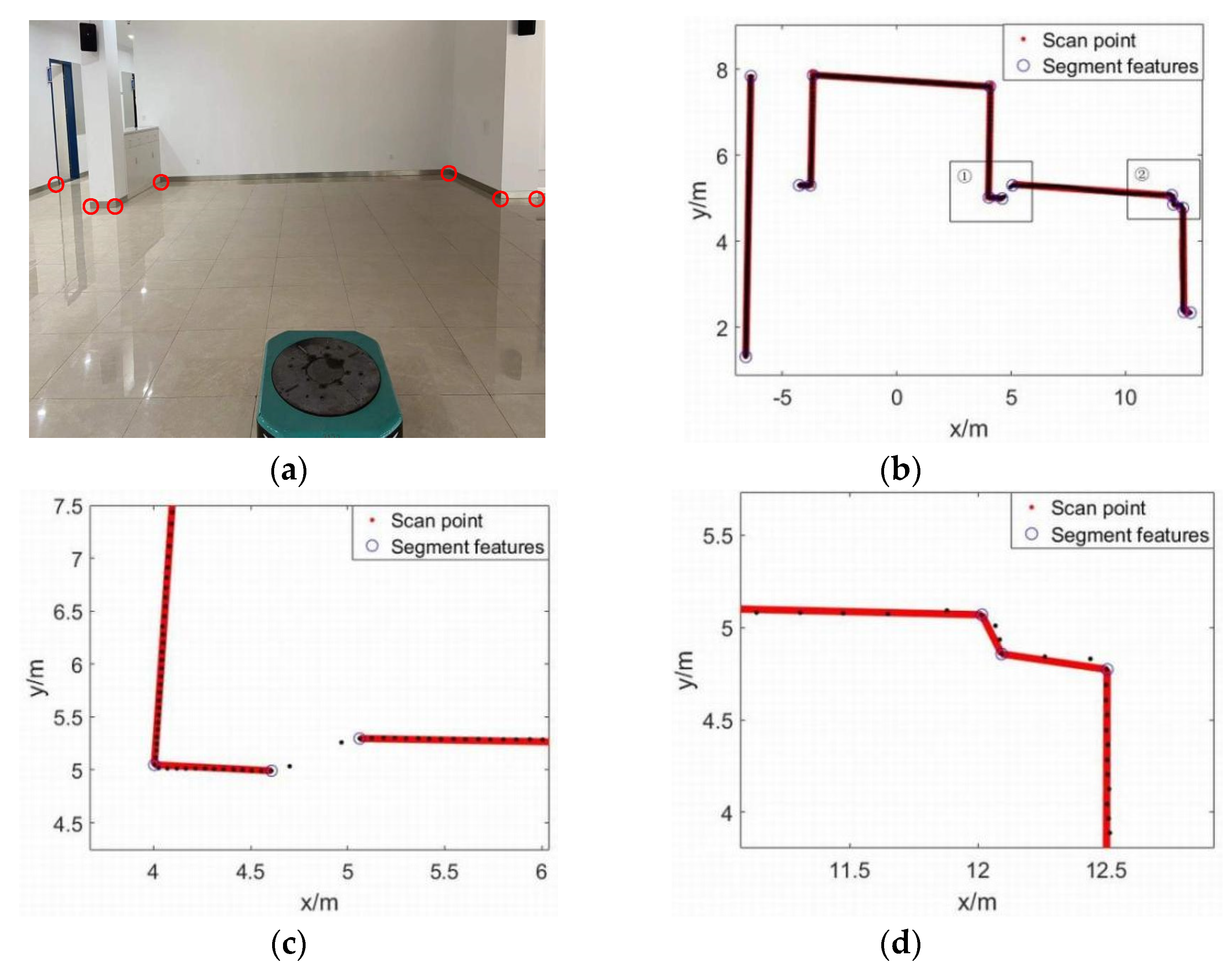
4.2. Real Environment Simulation

The simulation of the real environment uses the TIM 571 Lidar of SICK Company to collect environmental data. The specific parameters of the radar are shown in

Table 2. SICK TIM571 Parameters.

Parameter	Value
measurement range	0.05 m–25 m
scanning angle	160° (adjustable)
angular resolution	0.33°
scanning frequency	15 Hz
system error	±60 ms

.

In this study, the starting measurement angle of laser radar is 10°, the termination angle is 170°, and a total of 481 sets of data were collected. The algorithm uses Matlab 2016b simulation environment, the computer CPU is Intel Core i5-6300U, and memory is 8 GB. The experimental parameters are as follows: The data window size of mean filtering is N = 10, the amplification factor of breakpoint detection is k = 3, the range of corner extraction threshold dk_th is (0,0.052), and the weight of fitting error square (SSE) is W_i = 1.

Figure 8a shows the corridor environment, and the red points are the feautre points in the environment; Figure 8b is the line segment features extracted by this algorithm, of which six breakpoints and eight corner features were identified correctly. Figure 8c,d are the local amplification images of line segment extraction. Region 1 has breakpoints and corners corresponding to the right column in the corridor environment, and the right side of the column cannot be scanned by laser radar. Therefore, breakpoints will appear in line segment feature extraction, and different obstacles will be on both sides of the breakpoint. Region 2 has continuous corner points, where the data points of the original point set are distributed unevenly on the obstacle. The algorithm in this paper performs noise reduction processing to reduce over-segmentation. The experimental results show that the adaptive threshold segment extracted by this algorithm is ideal, and the line features at the details can be accurately extracted.

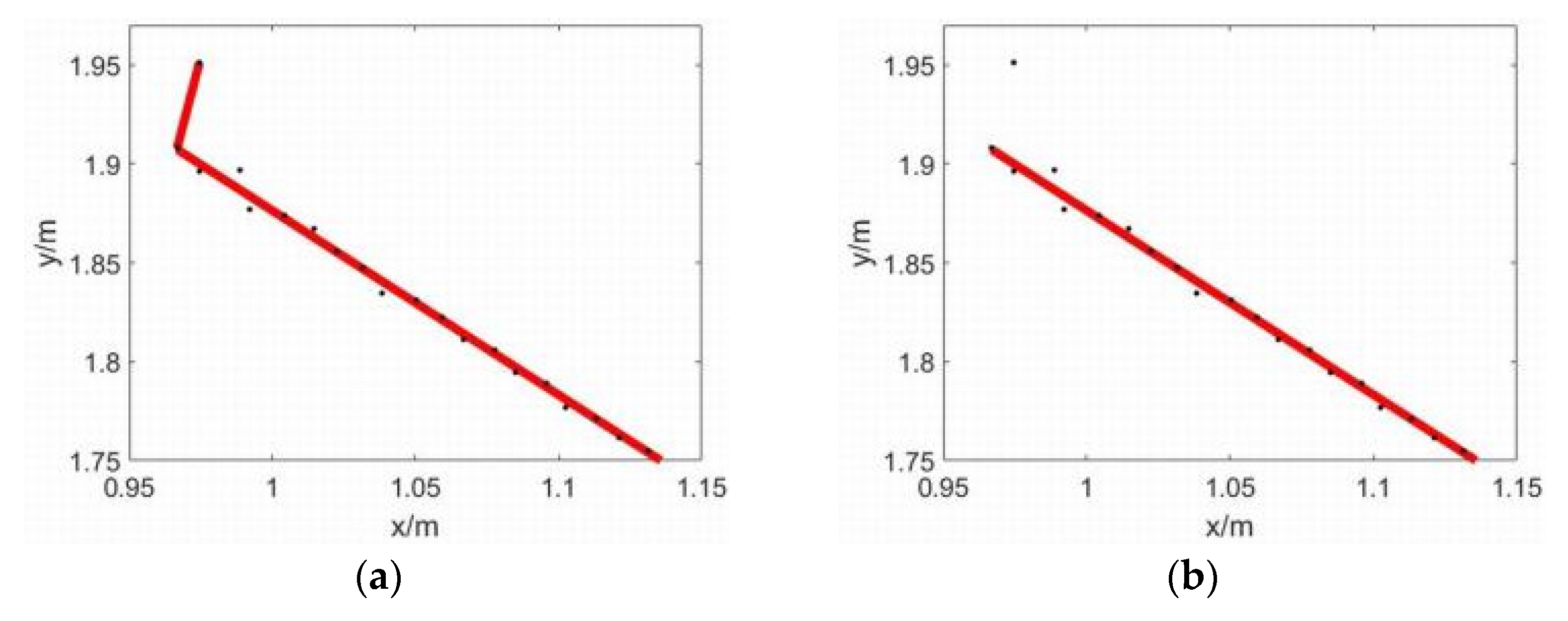
4.3. Fitting Contrast

Figure 9 is the line segment fitting results of the indoor environment. Figure 10, Figure 11 and Figure 12 are the fitting comparison of the three regions of Figure 9 using different algorithms.

In Figure 10a, the IEPF algorithm is used to extract the line segment feature of Region 1. Due to the uneven distribution of data points on the line segment, the data points affected by noise are misjudged into corner points, and the over-segmentation caused by fixed threshold occurs. The fitting line is quite different from the real environment. In Figure 10b, the algorithm uses adaptive threshold segmentation point set; thus, no segmentation occurs.

In Figure 11a, the IEPF algorithm is used to extract the line segment feature of Region 2. Due to the mutation noise at the breakpoint which is not processed previously, the breakpoint in the real environment is judged as an angle point wrongly, and the mutation noise is judged as a breakpoint wrongly. In Figure 11b, the proposed algorithm performs noise reduction on the original point set, and the line segment fitting results are correct.

In Figure 12a, PDBS algorithm is used to extract the line feature of Region 3. The PDBS algorithm uses a fixed threshold to segment the point set. The data points are dense at line 1, and the fixed threshold does not judge the corner point, resulting in under-segmentation, while over-segmentation occurs at line 2. In Figure 12b, line segment 1 and line segment 2 extracted by the proposed algorithm do not appear to experience over-segmentation or under-segmentation, and the line segment feature is highly matched with the real environment.

The experiments above show that the proposed algorithm has higher accuracy in the feature extraction of line segments than compared to the other two methods, and it fits real environment information better.

4.4. Calculation of Environmental Similarity

Figure 13 shows the environmental similarity error curves measured by the PDBS algorithm, IEPF algorithm, and the algorithm in this paper for the above indoor environment. The calculation basis of the similarity error is the vertical distance from all points on the point set to the fitting line. As shown in Figure 13a, the PDBS algorithm is too far from the fitting line of some feature points, and its similarity error is more than 0.02 m. Due to the existence of noise points at corners, the segmentation of point set is not incorrect, resulting in an uneven distribution of points on the fitting line segment. As shown in Figure 13b, the similarity error of IEPF algorithm fluctuates more, indicating that it often over-segments on the line segment and fitting fails due to noise interference. As shown in Figure 13c, the similarity error of this algorithm is less than 0.02 m, and the similarity error fluctuation is small. It is less affected by noise interference, which reduces the occurrence of over-segmentation and under-segmentation, and the similarity is 8.3% higher than that of the IEPF algorithm.

4.5. Feature Point Extraction Results and Algorithm Time

In the experiment, 10 frames of point cloud information in different indoor environments are extracted by using 2D laser radar, and line segment feature extraction is performed. The number of extracted breakpoints and corner points is shown in

Table 3. Comparison of Feature Point Extraction Results.

Number	Actual Number of Breakpoints	Actual Number of Cornerpoints	Number of Breakpoints Extracted		Number of Cornerpoints Extracted		Accuracy Rate of Feature Point Extraction		Algorithm Time/ms
			IEPF Algorithm	Proposed Algorithm	IEPF Algorithm	Proposed Algorithm	IEPF Algorithm	Proposed Algorithm	IEPF Algorithm	Proposed Algorithm
1	6	8	6	6	10	8	85.71%	100%	23.3	5.7
2	8	4	8	9	4	4	100%	91.67%	19.4	4.6
3	7	8	7	7	11	8	80%	100%	24.6	5.1
4	12	6	9	12	7	7	77.78%	94.44%	21.4	4.9
5	6	11	5	6	11	11	94.12%	100%	26.9	6.8
6	5	18	6	5	19	16	91.30%	91.30%	39.7	9.2
7	3	10	3	3	12	10	84.62%	100%	22.6	5.6
8	5	6	5	5	6	6	100%	100%	20.1	4.7
9	2	7	2	2	8	7	88.89%	100%	20.6	5.2
10	8	9	7	8	10	8	88.24%	94.12%	26.3	6.9

. The results show that the extraction accuracy of line segment feature points by this algorithm is more than 90%, which reduces the problem of environmental map information loss caused by over-segmentation or under-segmentation. The efficiency of corner extraction from single frame scanning data is four times higher than that of the IEPF algorithm, which avoids recursive operations and improves the real-time performance of line fitting.

5. Conclusions

The optimal feature points cannot be obtained by using the fixed threshold segmentation point set, which leads to missing environmental information on the fitting line segment. Therefore, this paper proposes an adaptive threshold-based line segment feature extraction algorithm for laser radar scanning environments.

(1) In the noise reduction stage of radar data, mean filtering is used to process the data points with uneven distribution, which improves the smoothness of data.

(2) In the point set segmentation stage, for obstacles at different distances, the nearest neighbor algorithm with adaptive threshold is used to detect breakpoints. The method of slope difference to judge corner feature is given. The scanning points obtained in laser radar are used to correspond to the vector diameter’s length and angle. The slope difference of adjacent points is calculated to initial segment the point set. The fitting error square sum is used to evaluate the segmentation effect to obtain the optimal corner judgment threshold.

(3) Segmented points are fitted by least square method to obtain line segment features.

The experimental results show that the new algorithm in this paper can avoid recursive operation. The accuracy of feature points extracted for different indoor environments is above 90%. Compared with the IEPF (Iterative End Point Fit) algorithm, the environmental similarity increased by 8.3%, and efficiency increased by four times, which meets the real-time requirements of line segment fitting. The new algorithm ensures the real-time performance of mobile robot map construction, which is suitable for the autonomous robot mapping algorithm developed by the embedded system and serves for subsequent positioning and navigation. This paper focuses on the environmental feature extraction of laser radar data when the mobile robot is still. On this basis, removing laser radar distortion generated by the mobile robot is the main topic to be studied in the future.

References

1. Hui, Y.; Hao, Y.G.; Liu, J.M. Research on Multi-sensor Image Matching Algorithm Based on Improved Line Segments Feature. In Itm Web of Conferences; EDP Sciences: Les Ulis, France, 2017; Volume 11, p. 05001. [Google Scholar] [CrossRef] [Green Version]
2. Wang, X.; Zhang, J. An Improved Automatic Shape Feature Extraction Method Based on Template Matching. In Journal of Physics: Conference Series; IOP Publishing: Bristol, UK, 2021; Volume 2095. [Google Scholar] [CrossRef]
3. Zhao, Q. Research on Real-Time Navigation and Positioning Model and Method of Motion Platform Based on RGB-D Camera; University of Chinese Academy of Sciences (Institute of Remote Sensing and Digital Earth, Chinese Academy of Sciences): Guangzhou, China, 2017. [Google Scholar]
4. Rakita, D.; Mutlu, B.; Gleicher, M. Single-query Path Planning Using Sample-efficient Probability Informed Trees. IEEE Robot. Autom. Lett. 2021, 6, 4624–4631. [Google Scholar] [CrossRef] [PubMed]
5. Tao, B.; Wu, H.; Gong, Z.; Yin, Z.; Ding, H. An RFID-Based Mobile Robot Localization Method Combining Phase Difference and Readability. IEEE Trans. Autom. Sci. Eng. 2020, 18, 1–11. [Google Scholar] [CrossRef]
6. Sun, W.; Yuan, H.; Liu, N.; Liu, Q.; Shu, S. Fast registration algorithm for line laser point clouds with contour features. J. Electron. Meas. Instrum. 2021, 35, 156–162. [Google Scholar] [CrossRef]
7. Sandy; Zhou, J.; Huang, P.; Li, L. Hybrid algorithm for line segment feature extraction of laser SLAM autonomous navigation. Mech. Des. Manuf. 2021, 5, 264–268. [Google Scholar] [CrossRef]
8. Borges, G.A.; Aldon, M.J. Line extraction in 2D range images for mobile robotics. J. Intell. Robot. Syst. 2004, 40, 267–297. [Google Scholar] [CrossRef]
9. Li, D.; Zhang, K.; Xu, R.; Luo, Z.; Wu, J.; Gui, H. Feature extraction for map creation of laser navigation robot without reflector. China Mech. Eng. 2018, 29, 2733–2739. [Google Scholar] [CrossRef]
10. Castellanos, J.A.; Tardós, J.D. Laser-based segmentation and localization for a mobile robot. Robot. Manuf. Recent Trends Res. Appl. 1996, 6, 101–108. [Google Scholar]
11. Ng, C.-C.; Yap, M.H.; Costen, N.; Li, B. Wrinkle Detection Using Hessian Line Tracking. IEEE Access 2015, 3, 1079–1088. [Google Scholar] [CrossRef] [Green Version]
12. Lu, F.; Xu, Y.; Li, Y.; Su, Z.; Wang, R. Multi-view fusion target detection and recognition based on DSmT theory. Robot 2018, 40, 723–733. [Google Scholar] [CrossRef]
13. Li, W.; Wang, W. Geometric feature map extraction method of laser SLAM based on Hough transform. Mechatronics 2018, 24, 3–7. [Google Scholar] [CrossRef]
14. Zhang, L.; Zhang, Y.; Zhenzhong, C.H.E.N.; Peipei, X.I.A.O.; Bin, L.U.O. Splitting and Merging Based Multi-model Fitting for Point Cloud Segmentation. J. Geod. Geoinf. Sci. 2019, 2, 78–89. [Google Scholar] [CrossRef]
15. Pu, L.; Xv, J.; Deng, F. An Automatic Method for Tree Species Point Cloud Segmentation Based on Deep Learning. J. Indian Soc. Remote Sens. 2021, 49, 1–10. [Google Scholar] [CrossRef]
16. Duda, R.O.; Hart, P.E. Pattern Classification and Scene Analysis; IEEE: New York, NY, USA, 1974; Volume 19, pp. 462–463. [Google Scholar] [CrossRef]
17. Wang, Y.S.; Qi, Y.; Man, Y. An Improved Hough Transform Method for Detecting Forward Vehicle and Lane in Road. In Journal of Physics: Conference Series; IOP Publishing: Bristol, UK, 2021; Volume 1757, p. 012082. [Google Scholar] [CrossRef]
18. Chen, W.; Jia, C. Artificial intelligence technology of laser imaging radar image edge detection. Laser Mag. 2020, 41, 85–88. [Google Scholar] [CrossRef]
19. He, Y.; Dong, L.; Zeng, F.; Dong, C.; Yao, J. Power Lines Extraction Using UVA LiDAR Point Clouds in Complex Terrains and Geological Structures. In IOP Conference Series: Earth and Environmental Science; IOP Publishing: Bristol, UK, 2021; Volume 804, pp. 032053–032058. [Google Scholar] [CrossRef]
20. Ravankar, A.A.; Ravankar, A.; Emaru, T.; Kobayashi, Y. Line Segment Extraction and Polyline Mapping for Mobile Robots in Indoor Structured Environments Using Range Sensors. SICE J. Control Meas. Syst. Integr. 2020, 13, 138–147. [Google Scholar] [CrossRef]
21. Yang, Y.; Yang, H.; Zhou, Z.; Yang, L. Research on High Voltage Power Line extraction based on Transmission Line Point Cloud characteristics and Model fitting. In IOP Conference Series: Earth and Environmental Science; IOP Publishing: Bristol, UK, 2020; Volume 446, pp. 042011–042018. [Google Scholar] [CrossRef]
22. Ma, Y.; Wei, Z.C.; Wang, Y. Point Cloud Feature Extraction Based Integrated Positioning Method for Unmanned Vehicle. Appl. Mech. Mater. 2014, 3276, 590. [Google Scholar] [CrossRef]
23. Lv, J.; Kobayashi, Y.; Ravankar, A.; Emaru, T. Straight line segments extraction and EKF-SLAM in indoor environment. J. Autom. Control Eng. 2014, 2, 270–276. [Google Scholar] [CrossRef]
24. An, S.Y.; Kang, J.G.; Lee, L.K.; Oh, S.Y. SLAM with salient line feature extraction in indoor environments. In Proceedings of the 2010 11th International Conference on Control Automation Robotics & Vision, Singapore, 7–10 December 2010; IEEE: New York, NY, USA, 2010. [Google Scholar]
25. Ravindranath, P.A.; Buyukburc, K.; Hasnain, A. Self-Calibration of Sensors Using Point Cloud Feature Extraction. In SPIE Future Sensing Technologies; International Society for Optics and Photonics: Bellingham, WA, USA, 2020. [Google Scholar] [CrossRef]
26. Xu, Z.; Shin, B.-S.; Klette, R. Accurate and Robust Line Segment Extraction Using Minimum Entropy With Hough Transform. IEEE Trans. Image Process. 2015, 24, 813–822. [Google Scholar] [CrossRef]
27. Li, H.; Liu, X.; Li, T.; Gan, R. A novel density-based clustering algorithm using nearest neighbor graph. Pattern Recognit. 2020, 102, 107206. [Google Scholar] [CrossRef]
28. Yang, Z.; Wang, C.; Zhou, L.; Yi, S. Line segment feature extraction method based on density clustering. Manuf. Autom. 2019, 41, 88–91. [Google Scholar]
29. Yu, C.; Ji, F.; Xue, J. Cutting Plane Based Cylinder Fitting Method With Incomplete Point Cloud Data for Digital Fringe Projection. IEEE Access 2020, 8, 149385–149401. [Google Scholar] [CrossRef]
30. Gao, X.; Jiang, L.; Wang, H.; Wang, X. Laser radar line feature extraction algorithm combined with SVM. Comput. Eng. Des. 2019, 40, 2384–2388. [Google Scholar] [CrossRef]
31. Liu, P.; Ren, G.; He, Z. The extraction method of feature corners in 2D laser SLAM. J. Nanjing Univ. Aeronaut. Astronaut. 2021, 53, 366–372. [Google Scholar] [CrossRef]
32. Slam Benchmarking. Available online: http://ais.informatik.uni-freiburg.de/slamevaluation/datasets.php (accessed on 24 May 2022).
Figure 1. Radar ranging model.
Electronics 11 01759 g001
Figure 2. Data preprocessing: (a) Radar raw data point set and the point set after denoising; (b) radar raw data adjacent point distance and the distance between adjacent points after denoising.
Electronics 11 01759 g002
Figure 3. Breakpoint feature: (a) Lidar data points; (b) distance between adjacent points.
Electronics 11 01759 g003
Figure 4. Comparison of breakpoint detection effect under the same k value: (a) k = 1; (b) k = 3; (c) k = 5; (d) k = 10.
Electronics 11 01759 g004
Figure 5. Schematic diagram of the scanning point.
Electronics 11 01759 g005
Figure 6. (a) Δk(i) after data point calculation; (b) distribution diagram at corner Δk(i).
Electronics 11 01759 g006
Figure 7. Simulation results of open-source datasets in Intel Research Laboratory: (a) multi breakpoint environment; (b) multi-angle environment.
Electronics 11 01759 g007
Figure 8. Line segment feature extraction example: (a) corridor environment; (b) overall graph of line segment feature extraction; (c) local amplification of region 1; (d) local amplification of region 2.
Electronics 11 01759 g008
Figure 9. Line fitting graph of this algorithm.
Electronics 11 01759 g009
Figure 10. Area 1 line fitting results: (a) IEPF algorithm; (b) proposed algorithm.
Electronics 11 01759 g010
Figure 11. Area 2 line fitting results: (a) IEPF algorithm; (b) proposed algorithm.
Electronics 11 01759 g011
Figure 12. Area 3 line fitting results: (a) PDBS algorithm; (b) proposed algorithm.
Electronics 11 01759 g012
Figure 13. Environmental similarity error curves of different algorithms: (a) PDBS algorithm; (b) IEPF algorithm; (c) Proposed algorithm.
Electronics 11 01759 g013