
Automatic Classification of Hospital Settings through Artificial Intelligence


Abstract
:1. Introduction
1.1. Related Works
1.2. The Role of Artificial Intelligence
1.3. Novelty of the Proposed Approach
- We analysed and compared three general models for environment classification: Google Vision API, Microsoft Azure Cognitive Services and the Clarifai General Model;
- We then created a customised model that was specifically trained for our needs using the Clarifai Custom Model;
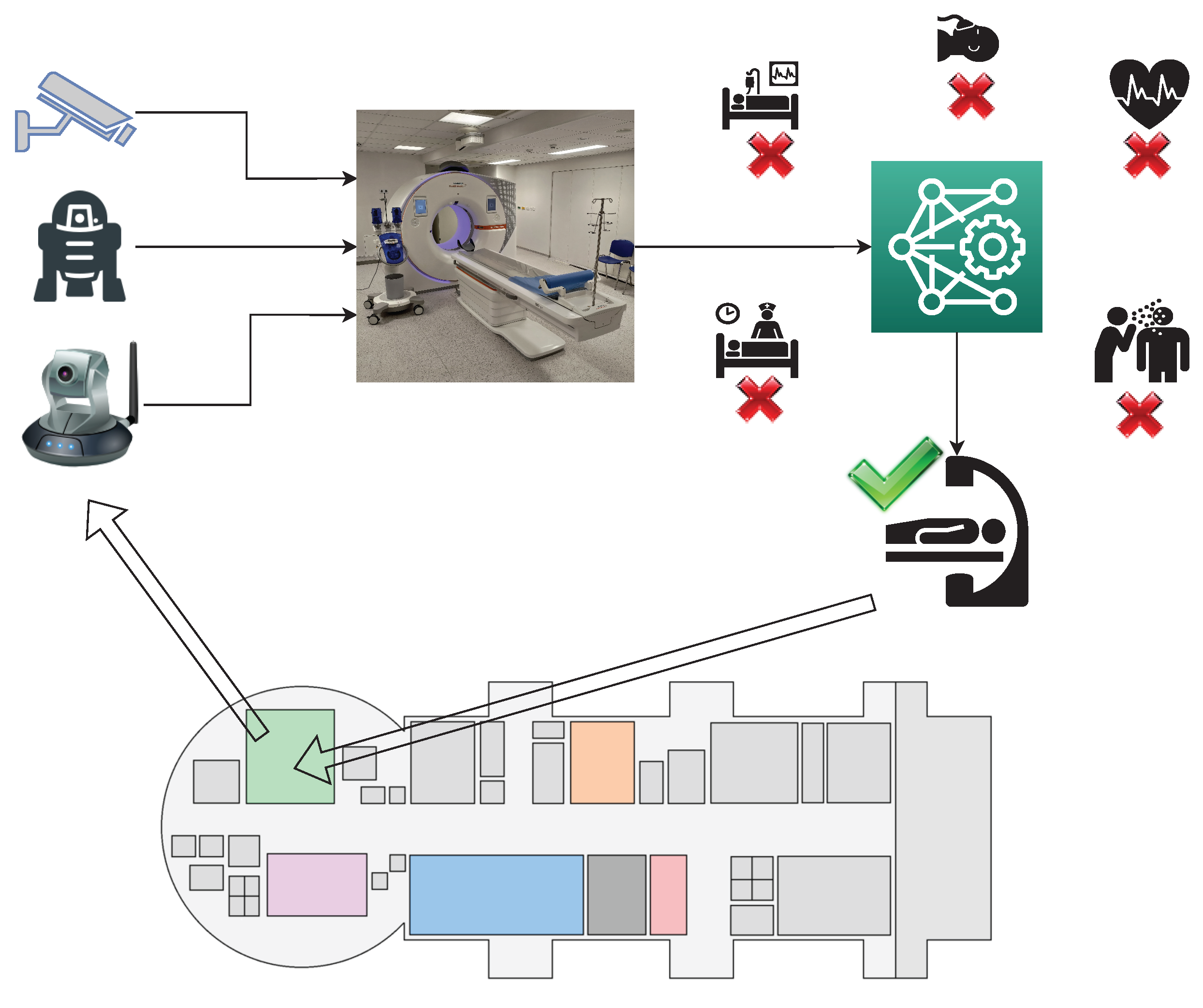
- Finally, we carried out one last type of classification using Detectron2, an object detection software that works in combination with an RF classifier for image recognition.
2. Materials and Methods
2.1. Datasets
2.1.1. First Dataset
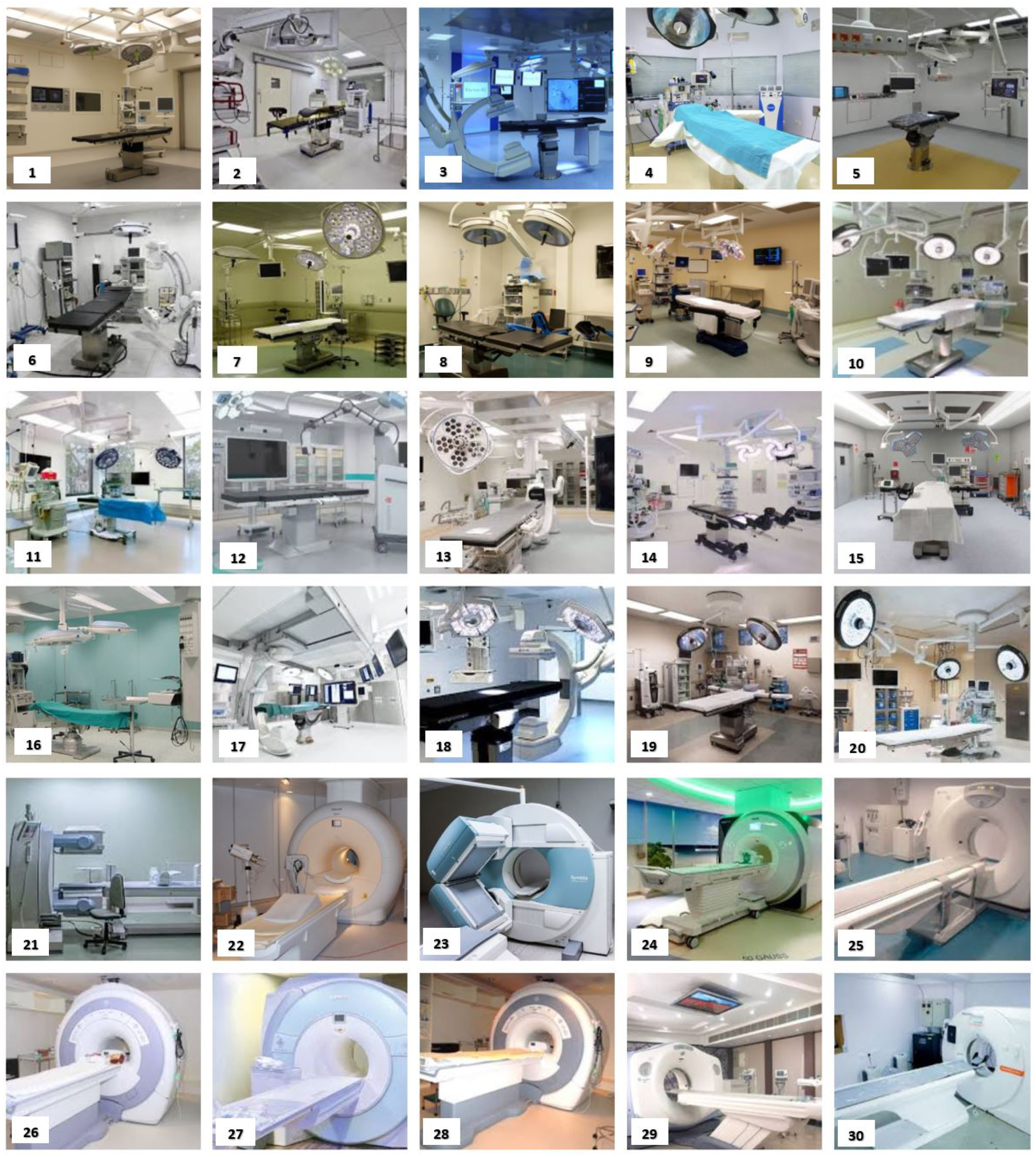
- 20 “surgery” images (from 1 to 20);
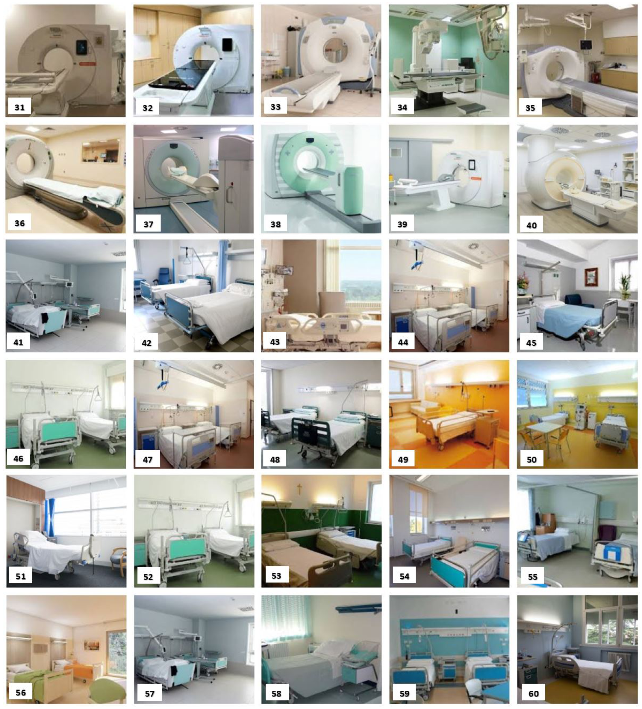
- 20 images of “diagnostic and therapeutic radiology” (from 21 to 40);
- 20 “hospitalisation” images (from 41 to 60);
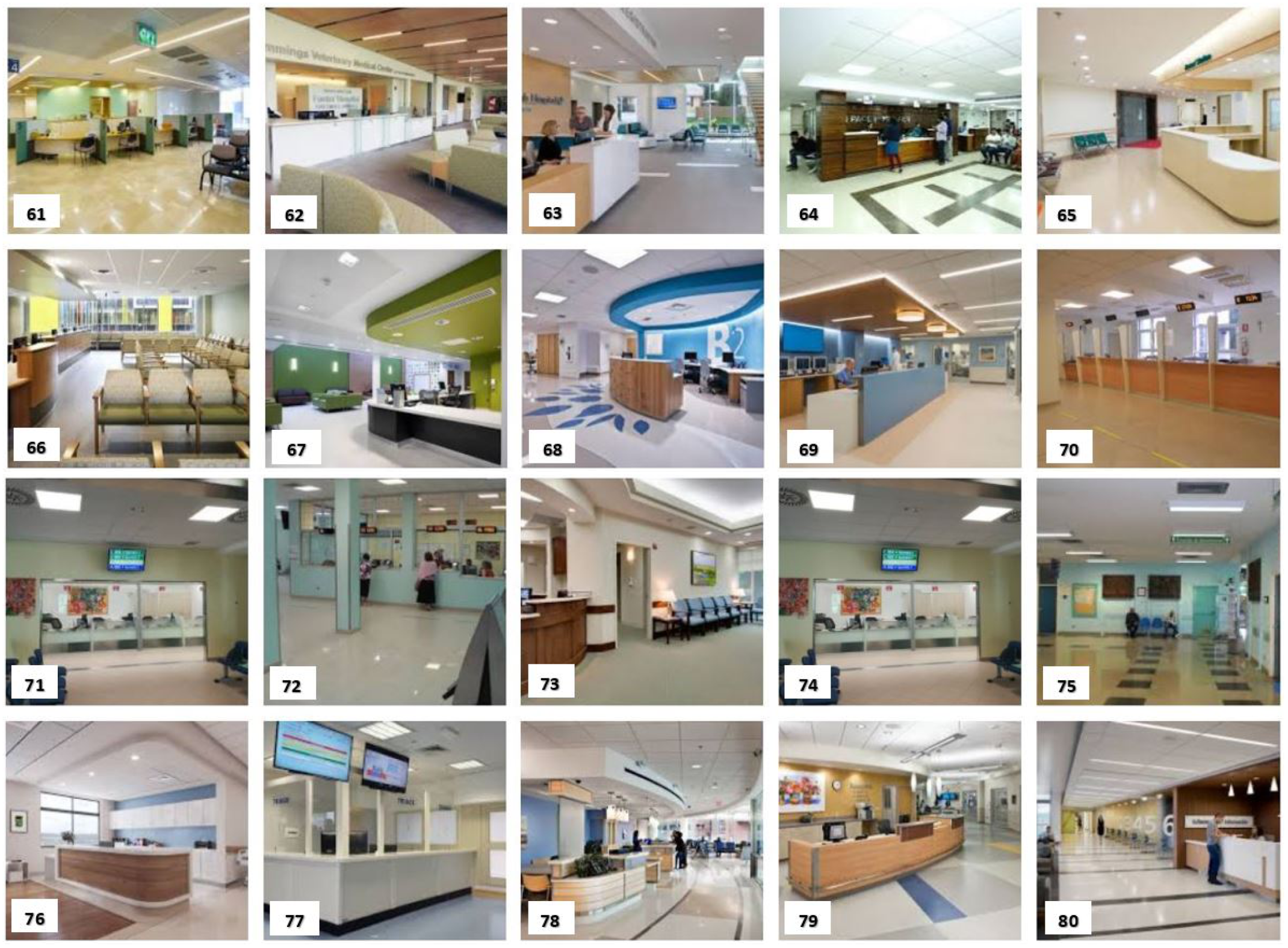
- 20 “acceptance” images (from 61 to 80).
- The training set, which was only used during the model training phase. This set was composed of images that were divided into two groups:
- –
- Positive examples, i.e., photographs for each of the four classes that were introduced as positive benchmark examples;
- –
- Negative examples, i.e., photographs of negative examples that were imported for each of the four classes from the remaining IUs.
- The test set, which was used in the model performance verification phase. This was made up of 40 images from the four chosen IUs.
- The first version comprised 10 positive examples and 18 negative examples for each IU (6 images for each incorrect IU);
- The second version comprised 20 positive examples and 18 negative examples for each IU (6 images for each incorrect IU).
- Items 21, 22, 23, 24, 25 and 26 (from the “diagnostic and therapeutic radiology” IU);
- Items 41, 42, 43, 44, 45 and 46 (from the “hospitalisation” IU);
- Items 61, 62, 63, 64, 65 and 66 (from the “acceptance” IU).
2.1.2. Second Dataset
- The first model examined “hospitalisation”, “radiology” and “surgery” rooms, for which 40 images per room were acquired from Google Images [61] using the corresponding keywords for a total of 120 images in the first dataset;
- The second model included six more IUs (“ambulance”, “analysis laboratory”, “intensive therapy”, “medical clinic”, “rehabilitation and physiotherapy” and “toilet”) for a total of nine hospital settings, for which 40 images per room were selected from Google Images [61] using the corresponding keywords for a total of 360 images in the second dataset.
- The training Set, which was composed of 25 images per IU and was used to train the algorithm to recognise the objects of interest;
- The validation Set, which was composed of 10 images per IU and was used to refine the hyperparameters of the model during training;
- The test Set, which was composed of the remaining 5 images per IU and was used at the end of the training to produce a final evaluation of the model.
2.2. Models Based on Image Understanding Services: General Classification Models
2.3. Models Customised through Transfer Learning
Implementation of the Customised Models
2.4. Combined Use of Detectron2 and an RF Classification Algorithm
2.4.1. Dataset Pre-Processing
- The first version contained the dataset without modifications: 75 training images, 30 validation images and 15 test images for the first model; 225 training images, 90 validation images and 45 test images for the second model;
- The second version contained the modified dataset, with an image rotation of up to ±45° and a blur of up to 1 pixel were applied (this choice was motivated by the size of the images that were downloaded from Google): 224 training images, 30 validation images and 15 test images for the first model; 671 training images, 90 validation images and 45 test images for the second model.
2.4.2. Parameter Selection and Model Calibration
Detectron2: Parameters and Calibration
- Average precision (AP) is the ratio between the true positives (correct answers) and the sum of the true positives and false positives (incorrect answers that are considered correct by the model). It indicates the percentage with which the model identifies an object. In the results, six types of average precision were considered, whose meaning is described in Table 6. Three APs were based on the intersection over union (IoU), which represents the overlap between the “predicted” and real bounding boxes. A bounding box is a box that is outlined around the object of interest in order to locate it within the image. The IoU is calculated as the intersection area of the union area of these two cited bounding boxes. A value of 1 represents a perfect overlap.
- Average recall is the ratio between the true positives and the sum of the true positives and false negatives (correct answers but considered wrong by the model). It indicates the percentage with which the model correctly identifies an object.
- Total loss evaluates the model’s behaviour with the datasets: the lower the value, the better the behaviour. It is calculated during the training and validation phases.
RF Classifier: Parameters and Calibration
- Accuracy is the ratio of correctly predicted observations to the total observations, i.e., (TP + TN)/(TP + TN + FP + FN);
- Score is the harmonic mean between precision and recall (which is usually more useful than accuracy, especially for non-symmetrical datasets and when the costs of false positives and false negatives are very different), i.e., 2 * ((precision * recall)/(precision + recall));
- Precision is the ratio of correctly predicted positive observations to the total predicted positive observations (the higher the value, the lower the number of false positives), i.e., TP/(TP + FP);
- Recall or TPR is the ratio of correctly predicted positive observations to all truly positive observations, i.e., TP/(TP + FN);
- Specificity is the ratio of correctly predicted negative observations to the total negative observations, i.e., TN/(TN + FP);
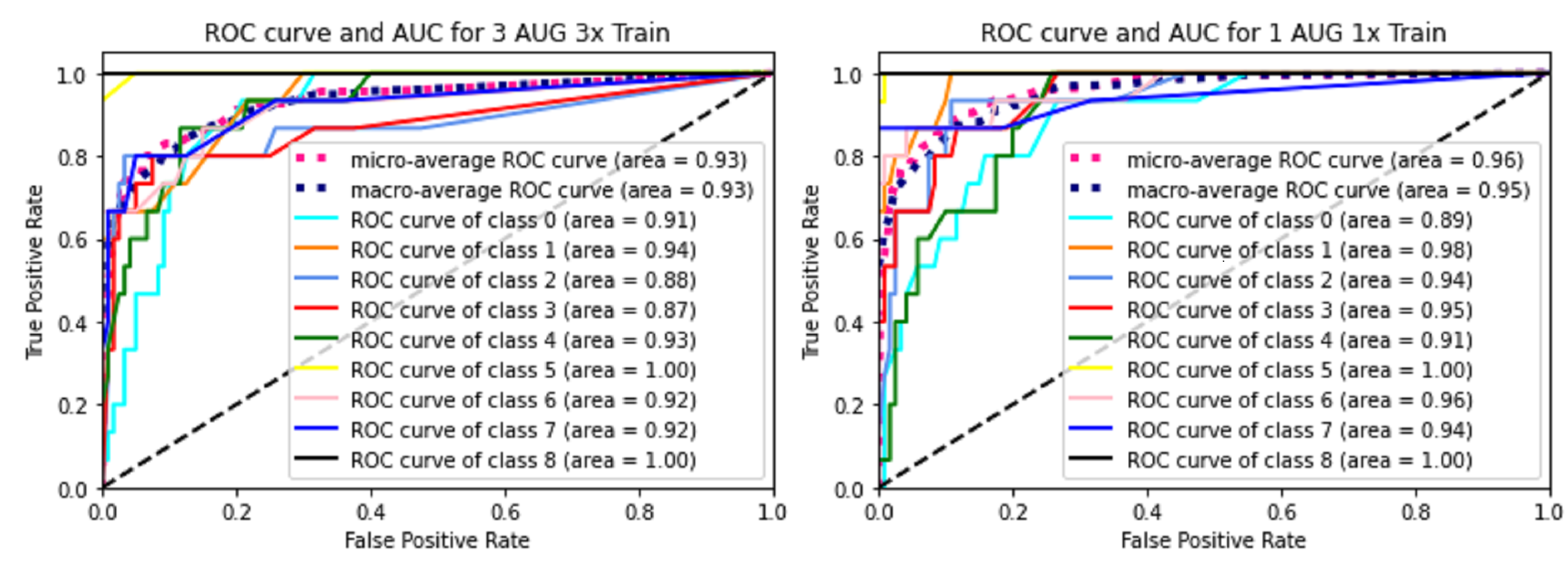
- The receiver operating characteristic curve (ROC curve) is a graph showing the diagnostic capability of a binary classification system as a function of its discrimination thresholds, which plots the true positive rate (TPR) versus the false positive rate (FPR = 1 − TPR) at different threshold settings;
- The area under the ROC curve (ROC AUC score) is the area under the ROC curve, which equals 1 when the classifier works perfectly.
3. Results
3.1. Comparison of the General Models of Cloud Services
3.2. Results Obtained with the Clarifai Custom Model
3.3. Results from the Combined Use of Detectron2 and the RF Classification Algorithm
3.3.1. Performance Obtained with the First Model
3.3.2. Performance Obtained with the Second Model
4. Discussion of Results
4.1. Discussion of Results Obtained with General Models and the Clarifai Custom Model
4.2. Discussion of Results Obtained with the Combined Use of Detectron2 and the RF Classification Algorithm
5. Conclusions
Author Contributions
Funding
Conflicts of Interest
Abbreviations
| AI | Artificial Intelligence |
| AP | Average Precision |
| API | Applicant Program Interface |
| BIM | Building Information Modelling |
| CAFM | Computer-Aided Facility Management |
| CNN | Convolutional Neural Network |
| CSAIL | Computer Science and Artificial Intelligence Laboratory |
| DBMS | Database Management System |
| DL | Deep Learning |
| FAIR | Facebook Artificial Intelligence Research |
| GIS | Graphical User Interface |
| GPU | Graphics Processing Unit |
| IoU | Intersection Over Union |
| IT | Information Technology |
| IU | Intended Use |
| JSON | JavaScript Object Notation |
| ML | Machine Learning |
| OCR | Optical Character Recognition |
| RF | Random Forest |
| ROC Curve | Receiver Operating Characteristic Curve |
| ROC AUC Score | Area Under the ROC Curve Score |
| TL | Transfer Learning |
Appendix A
- Photographs 1–10 in Figure A1: positive examples of the training set used for both versions of the custom model for the “surgery” IU;
- Photographs 11–20 in Figure A1: test set used for both versions of the custom model for the “surgery” IU;
- Photographs 21–30 in Figure A1: positive examples of the training set used for both versions of the custom model for the “diagnostic and therapeutic radiology” IU;
- Photographs 31–40 in Figure A2: test set used for both versions of the custom model for the “diagnostic and therapeutic radiology” IU;
- Photographs 41–50 in Figure A2: positive examples of the training set used for both versions of the custom model for the “hospitalisation” IU;
- Photographs 51–60 in Figure A2: test set used for both versions of the custom model for the “hospitalisation” IU;
- Photographs 61–70 in Figure A3: positive examples of the training set used for both versions of the custom model for the “acceptance” IU;
- Photographs 71–80 in Figure A3: test set used for both versions of the custom model for the “acceptance” IU.


Appendix B
- Table A1 refers to the “surgery” IU and the results that were obtained with Google Vision API;
- Table A2 refers to the “radiology” IU and the results that were obtained with the Clarifai General Model;
- Table A3 refers to the “hospitalisation” IU and the results that were obtained with Microsoft Azure Cognitive Services;
- Table A4 refers to the “acceptance” IU and the results that were obtained with Google Vision API.

| Im. 1 | Im. 2 | Im. 3 | Im. 4 | Im. 5 | Im. 6 | Im. 7 | Im. 8 | Im. 9 | Im. 10 | Im. 11 | Im. 12 | Im. 13 | Im. 14 | Im. 15 | Im. 16 | Im. 17 | Im. 18 | Im. 19 | Im. 20 | |
|---|---|---|---|---|---|---|---|---|---|---|---|---|---|---|---|---|---|---|---|---|
| Hospital | 93% | 97% | / | 98% | 79% | 95% | 94% | 95% | 96% | 97% | 97% | 97% | 97% | 91% | 89% | 96% | 92% | 92% | 86% | 96% |
| Medical Equipment | 91% | 97% | 81% | 94% | / | 97% | 96% | 98% | 92% | 98% | 97% | 97% | 98% | 95% | 94% | 96% | 96% | / | 89% | 98% |
| Room | 93% | 91% | 83% | 95% | 92% | 84% | 94% | 94% | 89% | 93% | 95% | 93% | 92% | 92% | 85% | 96% | 86% | 81% | 89% | 92% |
| Operating Theater | 96% | 90% | / | 96% | 79% | 63% | 98% | 98% | 87% | 96% | 77% | 78% | 88% | 57% | 70% | 98% | 55% | 83% | 89% | 90% |
| Medical | 64% | 80% | / | 86% | / | 92% | 85% | 94% | 76% | 96% | 88% | 90% | 95% | 59% | / | 88% | 79% | 96% | 77% | 93% |
| Im. 21 | Im. 22 | Im. 23 | Im. 24 | Im. 25 | Im. 26 | Im. 27 | Im. 28 | Im. 29 | Im. 30 | Im. 31 | Im. 32 | Im. 33 | Im. 34 | Im. 35 | Im. 36 | Im. 37 | Im. 38 | Im. 39 | Im. 40 | |
|---|---|---|---|---|---|---|---|---|---|---|---|---|---|---|---|---|---|---|---|---|
| Hospital | 99.5% | 99.2% | 94.3% | 97.5% | 98.8% | 99.4% | 93.8% | 99.2% | 98.7% | 97.9% | 99.4% | 96.3% | 99.3% | 99.8% | 98.4% | 98.8% | 98.1% | 85.8% | 99.4% | 99.0% |
| Medicine | 99.3% | 99.1% | 96.6% | 98.0% | 98.8% | 99.4% | 97.6% | 99.0% | 95.7% | 98.5% | 99.5% | 98.0% | 99.0% | 99.7% | 97.5% | 98.1% | 98.4% | 96.7% | 99.5% | 98.9% |
| Equipment | 98.9% | / | 93.9% | 94.9% | 98.4% | 97.5% | 95.7% | 95.0% | 89.8% | 94.3% | 98.5% | 97.4% | 94.9% | 97.7% | 90.9% | 93.3% | / | 97.0% | 97.1% | / |
| Clinic | 98.8% | / | 85.8% | 94.6% | 97.0% | 99.0% | 92.3% | 98.1% | 96.2% | 97.3% | 98.4% | 93.6% | 98.5% | 98.3% | 94.5% | 97.7% | / | 81.6% | 98.7% | 96.3% |
| Surgery | 98.2% | 98.9% | 94.9% | 95.9% | 98.3% | 97.2% | / | 98.2% | 97.4% | 93.2% | 98.0% | 93.4% | 95.2% | 99.8% | 95.3% | / | 94.4% | 86.0% | 97.6% | 97.0% |
| Room | 96.4% | 96.7% | / | / | / | 94.5% | 95.2% | 94.0% | 89.6% | 96.6% | 95.1% | / | 98.4% | 98.0% | 99.1% | 97.9% | 97.7% | / | 98.1% | 98.5% |
| Scrutiny | / | 91.3% | / | 91.8% | 92.5% | 97.3% | / | 96.7% | 97.0% | 95.9% | 97.2% | / | / | 97.9% | 93.0% | / | / | / | 95.7% | 94.1% |
| Radiography | / | 91.7% | / | / | / | 96.5% | / | / | / | / | 98.9% | / | / | 94.5% | / | / | 91.5% | / | 95.6% | / |
| Radiology | / | 90.8% | / | / | / | / | / | / | / | / | / | / | / | / | / | / | / | / | / | / |
| Diagnosis | / | 93.7% | 91.0% | / | / | / | / | / | / | / | / | / | / | / | / | / | / | / | / | 85.0% |
| Treatment | / | 88.5% | 86.0% | 91.6% | 91.6% | / | / | / | / | / | 95.7% | / | / | / | / | / | / | 82.7% | / | 90.2% |
| Emergency | / | / | 88.3% | / | / | / | / | / | / | / | / | / | / | / | / | / | / | / | / | / |
| Operating Room | / | / | / | / | / | / | / | / | / | / | / | / | / | 98.8% | / | / | / | / | / | / |
| Im. 41 | Im. 42 | Im. 43 | Im. 44 | Im. 45 | Im. 46 | Im. 47 | Im. 48 | Im. 49 | Im. 50 | Im. 51 | Im. 52 | Im. 53 | Im. 54 | Im. 55 | Im. 56 | Im. 57 | Im. 58 | Im. 59 | Im. 60 | |
|---|---|---|---|---|---|---|---|---|---|---|---|---|---|---|---|---|---|---|---|---|
| Medical Equipment | 96.2% | 95.7% | / | 92.6% | 55.5% | 97.3% | 92.6% | 94.6% | / | / | 86.6% | 97.8% | 92.7% | 74.0% | 87.2% | / | 92.7% | 84.7% | 95.0% | 66.1% |
| Furniture | 18.0% | 92.4% | 92.9% | 17.6% | 40.7% | 33.2% | 17.6% | 22.4% | 91.4% | 23.0% | 29.1% | 35.6% | 88.3% | 28.3% | 41.0% | 69.1% | 33.8% | 97.0% | 36.3% | 93.8% |
| Bedroom | 64.7% | 48.5% | / | / | 58.4% | / | / | / | / | / | 70.6% | / | 54.3% | 47.8% | 53.8% | 57.5% | 39.1% | 39.5% | / | 48.1% |
| Clinic | 51.5% | / | / | / | / | 63.9% | / | 54.4% | / | / | / | 68.9% | 52.4% | / | / | / | / | / | / | / |
| Hospital | 79.2% | 77.1% | / | 75.9% | / | 86.0% | 75.9% | 82.2% | / | / | 56.3% | 88.5% | 80.3% | / | 65.9% | / | 74.3% | 56.2% | 70.1% | / |
| Room | 76.4% | 55.4% | / | 72.0% | 96.2% | 76.0% | 72.0% | 80.4% | 73.2% | 84.0% | 90.3% | 43.5% | 77.5% | 41.0% | 92.2% | 93.3% | 78.7% | 53.5% | 77.1% | 81.8% |
| Hotel | / | / | / | / | 76.6% | / | / | / | 68.5% | / | / | / | 71.8% | 82.2% | / | 95.2% | / | / | / | 71.7% |
| Plumbing Fixture | / | / | / | / | / | / | / | / | / | / | / | / | / | / | / | / | / | / | / | 72.2% |
| Bathroom | / | / | / | 56.7% | / | / | 56.7% | / | 54.6% | / | / | / | / | / | / | 79.9% | / | / | / | 86.3% |
| House | / | / | / | 60.6% | 89.4% | / | 60.6% | / | / | 53.6% | / | / | / | 70.9% | / | 89.6% | / | / | / | 75.1% |
| Hospital Room | / | / | / | 77.0% | / | / | 77.0% | 60.4% | / | / | / | / | / | / | / | / | 82.1% | / | / | / |
| Office Building | / | / | / | / | / | / | / | 66.3% | / | 76.4% | / | / | / | / | / | / | / | / | 69.7% | / |
| Operating Theatre | / | / | / | / | / | 54.6% | / | / | / | / | / | 61.0% | / | / | / | / | / | / | / | / |
|
Im. 61 |
Im. 62 |
Im. 63 |
Im. 64 |
Im. 65 |
Im. 66 |
Im. 67 |
Im. 68 |
Im. 69 |
Im. 70 |
Im. 71 |
Im. 72 |
Im. 73 |
Im. 74 |
Im. 75 |
Im. 76 |
Im. 77 |
Im. 78 |
Im. 79 |
Im. 80 | |
|---|---|---|---|---|---|---|---|---|---|---|---|---|---|---|---|---|---|---|---|---|
| Room | 80% | 92% | 74% | 71% | 93% | 92% | 89% | 89% | 81% | 79% | 80% | 66% | 94% | 80% | 83% | 92% | 79% | 80% | 88% | 74% |
| Waiting Room | 66% | / | / | / | 76% | / | / | / | / | 82% | / | / | 89% | 65% | / | / | / | / | / | |
| Office | 56% | 87% | 89% | 61% | 71% | 59% | 88% | 92% | 92% | 51% | 60% | / | 84% | 56% | / | 90% | 60% | 89% | / | 88% |
| Hospital | / | / | 66% | / | 51% | / | / | / | / | / | 86% | 62% | / | 70% | 50% | / | / | / | / | / |
| Reception | / | / | / | / | / | / | / | / | / | / | / | / | / | / | / | / | / | / | 60% | / |
Appendix C
- Table A5 shows the dataset employed to test the three general models and the images are those that were used to train and test the two versions of the model described in Section 2.3;
- Table A6 describes the additional 40 images that were used for the second version of the model described in Section 2.3;
- Table A7 shows the dataset used for the first version of the Detectron2 model;
- Table A8 shows the dataset used for the second version of the Detectron2 model.
| IU | Name | Size (Pixel) | Horizontal | Vertical | Bit Depth |
|---|---|---|---|---|---|
| Resolution (dpi) | Resolution (dpi) | ||||
| Surgery | Image 1 | 640 × 427 | 72 | 72 | 24 |
| Image 2 | 275 × 183 | 96 | 96 | 24 | |
| Image 3 | 118 × 510 | 96 | 96 | 24 | |
| Image 4 | 880 × 586 | 96 | 96 | 24 | |
| Image 5 | 258 × 195 | 96 | 96 | 24 | |
| Image 6 | 275 × 183 | 96 | 96 | 24 | |
| Image 7 | 259 × 194 | 96 | 96 | 24 | |
| Image 8 | 487 × 325 | 72 | 72 | 24 | |
| Image 9 | 475 × 316 | 96 | 96 | 24 | |
| Image 10 | 275 × 183 | 96 | 96 | 24 | |
| Image 11 | 225 × 225 | 96 | 96 | 24 | |
| Image 12 | 273 × 185 | 96 | 96 | 24 | |
| Image 13 | 275 × 183 | 96 | 96 | 24 | |
| Image 14 | 225 × 225 | 96 | 96 | 24 | |
| Image 15 | 850 × 510 | 96 | 96 | 24 | |
| Image 16 | 550 × 413 | 96 | 96 | 24 | |
| Image 17 | 275 × 183 | 96 | 96 | 24 | |
| Image 18 | 341 × 148 | 96 | 96 | 24 | |
| Image 19 | 275 × 183 | 96 | 96 | 24 | |
| Image 20 | 304 × 166 | 96 | 96 | 24 | |
| Radiology | Image 21 | 275 × 183 | 96 | 96 | 24 |
| Image 22 | 2254 × 2056 | 72 | 72 | 24 | |
| Image 23 | 800 × 533 | 96 | 96 | 24 | |
| Image 24 | 267 × 189 | 96 | 96 | 24 | |
| Image 25 | 274 × 184 | 96 | 96 | 24 | |
| Image 26 | 270 × 187 | 96 | 96 | 24 | |
| Image 27 | 276 × 183 | 96 | 96 | 24 | |
| Image 28 | 259 × 194 | 96 | 96 | 24 | |
| Image 29 | 243 × 207 | 96 | 96 | 24 | |
| Image 30 | 275 × 183 | 96 | 96 | 24 | |
| Image 31 | 300 × 168 | 96 | 96 | 24 | |
| Image 32 | 281 × 180 | 96 | 96 | 24 | |
| Image 33 | 276 × 183 | 96 | 96 | 24 | |
| Image 34 | 225 × 225 | 96 | 96 | 24 | |
| Image 35 | 275 × 183 | 96 | 96 | 24 | |
| Image 36 | 286 × 176 | 96 | 96 | 24 | |
| Image 37 | 2048 × 1536 | 300 | 300 | 24 | |
| Image 38 | 245 × 206 | 96 | 96 | 24 | |
| Image 39 | 259 × 194 | 96 | 96 | 24 | |
| Image 40 | 870 × 575 | 96 | 96 | 24 | |
| Resolution (dpi) | Resolution (dpi) | ||||
| Hospitalisation | Image 41 | 800 × 600 | 96 | 96 | 24 |
| Image 42 | 700 × 525 | 72 | 72 | 24 | |
| Image 43 | 301 × 167 | 96 | 96 | 24 | |
| Image 44 | 275 × 183 | 96 | 96 | 24 | |
| Image 45 | 275 × 183 | 96 | 96 | 24 | |
| Image 46 | 299 × 168 | 96 | 96 | 24 | |
| Image 47 | 275 × 183 | 96 | 96 | 24 | |
| Image 48 | 275 × 183 | 96 | 96 | 24 | |
| Image 49 | 307 × 164 | 96 | 96 | 24 | |
| Image 50 | 275 × 183 | 96 | 96 | 24 | |
| Hospitalisation | Image 51 | 1000 × 667 | 96 | 96 | 24 |
| Image 52 | 299 × 168 | 96 | 96 | 24 | |
| Image 53 | 275 × 183 | 96 | 96 | 24 | |
| Image 54 | 275 × 183 | 96 | 96 | 24 | |
| Image 55 | 284 × 177 | 96 | 96 | 24 | |
| Image 56 | 270 × 187 | 96 | 96 | 24 | |
| Image 57 | 259 × 232 | 96 | 96 | 24 | |
| Image 58 | 259 × 194 | 96 | 96 | 24 | |
| Image 59 | 217 × 232 | 96 | 96 | 24 | |
| Image 60 | 1200 × 800 | 96 | 96 | 24 | |
| Acceptance | Image 61 | 275 × 183 | 96 | 96 | 24 |
| Image 62 | 259 × 194 | 96 | 96 | 24 | |
| Image 63 | 275 × 183 | 96 | 96 | 24 | |
| Image 64 | 275 × 183 | 96 | 96 | 24 | |
| Image 65 | 275 × 183 | 96 | 96 | 24 | |
| Image 66 | 270 × 187 | 96 | 96 | 24 | |
| Image 67 | 230 × 219 | 96 | 96 | 24 | |
| Image 68 | 274 × 184 | 96 | 96 | 24 | |
| Image 69 | 276 × 182 | 96 | 96 | 24 | |
| Image 70 | 252 × 200 | 96 | 96 | 24 | |
| Image 71 | 259 × 194 | 96 | 96 | 24 | |
| Image 72 | 259 × 194 | 96 | 96 | 24 | |
| Image 73 | 275 × 183 | 96 | 96 | 24 | |
| Image 74 | 512 × 384 | 96 | 96 | 24 | |
| Image 75 | 319 × 158 | 96 | 96 | 24 | |
| Image 76 | 290 × 174 | 96 | 96 | 24 | |
| Image 77 | 300 × 168 | 96 | 96 | 24 | |
| Image 78 | 255 × 197 | 96 | 96 | 24 | |
| Image 79 | 275 × 183 | 96 | 96 | 24 | |
| Image 80 | 275 × 183 | 96 | 96 | 24 |
| IU | Name | Size (Pixel) | Horizontal | Vertical | Bit Depth |
|---|---|---|---|---|---|
| Resolution (dpi) | Resolution (dpi) | ||||
| Surgery | Image 81 | 864 × 534 | 96 | 96 | 24 |
| Image 82 | 1600 × 1077 | 96 | 96 | 24 | |
| Image 83 | 288 × 175 | 96 | 96 | 24 | |
| Image 84 | 299 × 168 | 96 | 96 | 24 | |
| Image 85 | 275 × 183 | 96 | 96 | 24 | |
| Image 86 | 275 × 183 | 96 | 96 | 24 | |
| Image 87 | 289 × 175 | 96 | 96 | 24 | |
| Image 88 | 1800 × 1200 | 300 | 300 | 24 | |
| Image 89 | 261 × 193 | 96 | 96 | 24 | |
| Image 90 | 921 × 617 | 96 | 96 | 24 | |
| Radiology | Image 91 | 1024 × 576 | 72 | 72 | 24 |
| Image 92 | 800 × 450 | 72 | 72 | 24 | |
| Image 93 | 751 × 401 | 96 | 96 | 24 | |
| Image 94 | 1000 × 665 | 180 | 180 | 24 | |
| Image 95 | 259 × 194 | 96 | 96 | 24 | |
| Image 96 | 251 × 201 | 96 | 96 | 24 | |
| Image 97 | 225 × 225 | 96 | 96 | 24 | |
| Image 98 | 275 × 183 | 96 | 96 | 24 | |
| Image 99 | 300 × 168 | 96 | 96 | 24 | |
| Image 100 | 260 × 194 | 96 | 96 | 24 | |
| Hospitalisation | Image 101 | 600 × 338 | 72 | 72 | 24 |
| Image 102 | 986 × 657 | 96 | 96 | 24 | |
| Image 103 | 901 × 568 | 96 | 96 | 24 | |
| Image 104 | 1779 × 1192 | 300 | 300 | 24 | |
| Image 105 | 283 × 178 | 96 | 96 | 24 | |
| Image 106 | 1024 × 768 | 96 | 96 | 24 | |
| Image 107 | 667 × 500 | 96 | 96 | 24 | |
| Image 108 | 840 × 480 | 96 | 96 | 24 | |
| Image 109 | 259 × 194 | 96 | 96 | 24 | |
| Image 110 | 312 × 161 | 96 | 96 | 24 | |
| Acceptance | Image 111 | 194 × 259 | 96 | 96 | 24 |
| Image 112 | 279 × 180 | 96 | 96 | 24 | |
| Image 113 | 275 × 183 | 96 | 96 | 24 | |
| Image 114 | 276 × 183 | 96 | 96 | 24 | |
| Image 115 | 300 × 168 | 96 | 96 | 24 | |
| Image 116 | 374 × 135 | 96 | 96 | 24 | |
| Image 117 | 259 × 194 | 96 | 96 | 24 | |
| Image 118 | 301 × 168 | 96 | 96 | 24 | |
| Image 119 | 260 × 194 | 96 | 96 | 24 | |
| Image 120 | 259 × 194 | 96 | 96 | 24 |
| IU | Name | Size (Pixel) | Horizontal | Vertical | Bit Depth |
|---|---|---|---|---|---|
| Resolution (dpi) | Resolution (dpi) | ||||
| Hospitalisation | Image 1 | 297 × 170 | 96 | 96 | 24 |
| Image 2 | 264 × 191 | 96 | 96 | 24 | |
| Image 3 | 270 × 187 | 96 | 96 | 24 | |
| Image 4 | 275 × 183 | 96 | 96 | 24 | |
| Image 5 | 300 × 168 | 96 | 96 | 24 | |
| Image 6 | 276 × 183 | 96 | 96 | 24 | |
| Image 7 | 259 × 194 | 96 | 96 | 24 | |
| Image 8 | 310 × 163 | 96 | 96 | 24 | |
| Image 9 | 300 × 168 | 96 | 96 | 24 | |
| Image 10 | 285 × 177 | 96 | 96 | 24 | |
| Image 11 | 259 × 194 | 96 | 96 | 24 | |
| Image 12 | 275 × 183 | 96 | 96 | 24 | |
| Image 13 | 299 × 168 | 96 | 96 | 24 | |
| Image 14 | 275 × 183 | 96 | 96 | 24 | |
| Image 15 | 340 × 148 | 96 | 96 | 24 | |
| Image 16 | 314 × 160 | 96 | 96 | 24 | |
| Image 17 | 307 × 164 | 96 | 96 | 24 | |
| Image 18 | 194 × 259 | 96 | 96 | 24 | |
| Image 19 | 325 × 155 | 96 | 96 | 24 | |
| Image 20 | 259 × 194 | 96 | 96 | 24 | |
| Image 21 | 275 × 183 | 96 | 96 | 24 | |
| Image 22 | 361 × 140 | 96 | 96 | 24 | |
| Image 23 | 314 × 161 | 96 | 96 | 24 | |
| Image 24 | 275 × 183 | 96 | 96 | 24 | |
| Image 25 | 275 × 183 | 96 | 96 | 24 | |
| Image 26 | 276 × 183 | 96 | 96 | 24 | |
| Image 27 | 275 × 183 | 96 | 96 | 24 | |
| Image 28 | 259 × 194 | 96 | 96 | 24 | |
| Image 29 | 275 × 183 | 96 | 96 | 24 | |
| Image 30 | 275 × 183 | 96 | 96 | 24 | |
| Image 31 | 275 × 183 | 96 | 96 | 24 | |
| Image 32 | 260 × 194 | 96 | 96 | 24 | |
| Image 33 | 261 × 193 | 96 | 96 | 24 | |
| Image 34 | 275 × 183 | 96 | 96 | 24 | |
| Image 35 | 275 × 183 | 96 | 96 | 24 | |
| Image 36 | 274 × 184 | 96 | 96 | 24 | |
| Image 37 | 275 × 183 | 96 | 96 | 24 | |
| Image 38 | 300 × 168 | 96 | 96 | 24 | |
| Image 39 | 275 × 183 | 96 | 96 | 24 | |
| Image 40 | 275 × 183 | 96 | 96 | 24 | |
| Radiology | Image 1 | 257 × 196 | 96 | 96 | 24 |
| Image 2 | 275 × 183 | 96 | 96 | 24 | |
| Image 3 | 261 × 193 | 96 | 96 | 24 | |
| Image 4 | 233 × 216 | 96 | 96 | 24 | |
| Image 5 | 259 × 194 | 96 | 96 | 24 | |
| Image 6 | 300 × 168 | 96 | 96 | 24 | |
| Image 7 | 292 × 173 | 96 | 96 | 24 | |
| Image 8 | 311 × 162 | 96 | 96 | 24 | |
| Image 9 | 299 × 168 | 96 | 96 | 24 | |
| Image 10 | 273 × 185 | 96 | 96 | 24 | |
| Image 11 | 290 × 174 | 96 | 96 | 24 | |
| Image 12 | 275 × 183 | 96 | 96 | 24 | |
| Image 13 | 300 × 168 | 96 | 96 | 24 | |
| Image 14 | 259 × 194 | 96 | 96 | 24 | |
| Image 15 | 301 × 168 | 96 | 96 | 24 | |
| Image 16 | 270 × 187 | 96 | 96 | 24 | |
| Image 17 | 183 × 275 | 96 | 96 | 24 | |
| Image 18 | 299 × 168 | 96 | 96 | 24 | |
| Image 19 | 356 × 141 | 96 | 96 | 24 | |
| Image 20 | 270 × 186 | 96 | 96 | 24 | |
| Image 21 | 300 × 168 | 96 | 96 | 24 | |
| Image 22 | 308 × 164 | 96 | 96 | 24 | |
| Image 23 | 304 × 166 | 96 | 96 | 24 | |
| Image 24 | 275 × 183 | 96 | 96 | 24 | |
| Image 25 | 275 × 183 | 96 | 96 | 24 | |
| Image 26 | 300 × 168 | 96 | 96 | 24 | |
| Image 27 | 251 × 201 | 96 | 96 | 24 | |
| Image 28 | 283 × 178 | 96 | 96 | 24 | |
| Image 29 | 259 × 194 | 96 | 96 | 24 | |
| Image 30 | 301 × 168 | 96 | 96 | 24 | |
| Image 31 | 300 × 168 | 96 | 96 | 24 | |
| Image 32 | 299 × 168 | 96 | 96 | 24 | |
| Image 33 | 271 × 186 | 96 | 96 | 24 | |
| Image 34 | 248 × 203 | 96 | 96 | 24 | |
| Image 35 | 244 × 206 | 96 | 96 | 24 | |
| Image 36 | 244 × 206 | 96 | 96 | 24 | |
| Image 37 | 276 × 183 | 96 | 96 | 24 | |
| Image 38 | 299 × 168 | 96 | 96 | 24 | |
| Image 39 | 288 × 175 | 96 | 96 | 24 | |
| Image 40 | 302 × 167 | 96 | 96 | 24 | |
| Surgery | Image 1 | 275 × 183 | 96 | 96 | 24 |
| Image 2 | 275 × 183 | 96 | 96 | 24 | |
| Image 3 | 168 × 188 | 96 | 96 | 24 | |
| Image 4 | 292 × 173 | 96 | 96 | 24 | |
| Image 5 | 240 × 210 | 96 | 96 | 24 | |
| Image 6 | 275 × 183 | 96 | 96 | 24 | |
| Image 7 | 291 × 173 | 96 | 96 | 24 | |
| Image 8 | 275 × 183 | 96 | 96 | 24 | |
| Image 9 | 318 × 159 | 96 | 96 | 24 | |
| Image 10 | 194 × 259 | 96 | 96 | 24 | |
| Image 11 | 259 × 194 | 96 | 96 | 24 | |
| Image 12 | 269 × 187 | 96 | 96 | 24 | |
| Image 13 | 256 × 197 | 96 | 96 | 24 | |
| Image 14 | 300 × 168 | 96 | 96 | 24 | |
| Image 15 | 254 × 198 | 96 | 96 | 24 | |
| Image 16 | 324 × 155 | 96 | 96 | 24 | |
| Image 17 | 259 × 194 | 96 | 96 | 24 | |
| Image 18 | 258 × 195 | 96 | 96 | 24 | |
| Image 19 | 318 × 159 | 96 | 96 | 24 | |
| Image 20 | 259 × 194 | 96 | 96 | 24 | |
| Image 21 | 275 × 183 | 96 | 96 | 24 | |
| Image 22 | 286 × 176 | 96 | 96 | 24 | |
| Image 23 | 275 × 183 | 96 | 96 | 24 | |
| Image 24 | 258 × 195 | 96 | 96 | 24 | |
| Image 25 | 300 × 168 | 96 | 96 | 24 | |
| Image 26 | 264 × 191 | 96 | 96 | 24 | |
| Image 27 | 299 × 168 | 96 | 96 | 24 | |
| Image 28 | 295 × 171 | 96 | 96 | 24 | |
| Image 29 | 259 × 194 | 96 | 96 | 24 | |
| Image 31 | 340 × 148 | 96 | 96 | 24 | |
| Image 32 | 274 × 184 | 96 | 96 | 24 | |
| Image 33 | 275 × 183 | 96 | 96 | 24 | |
| Image 34 | 329 × 153 | 96 | 96 | 24 | |
| Image 35 | 275 × 183 | 96 | 96 | 24 | |
| Image 36 | 275 × 183 | 96 | 96 | 24 | |
| Image 37 | 259 × 194 | 96 | 96 | 24 | |
| Image 38 | 259 × 194 | 96 | 96 | 24 | |
| Image 39 | 251 × 201 | 96 | 96 | 24 | |
| Ambulance | Image 1 | 275 × 183 | 96 | 96 | 24 |
| Image 2 | 229 × 220 | 96 | 96 | 24 | |
| Image 3 | 275 × 183 | 96 | 96 | 24 | |
| Image 4 | 276 × 183 | 96 | 96 | 24 | |
| Image 5 | 300 × 168 | 96 | 96 | 24 | |
| Image 6 | 194 × 259 | 96 | 96 | 24 | |
| Image 7 | 244 × 206 | 96 | 96 | 24 | |
| Image 8 | 274 × 184 | 96 | 96 | 24 | |
| Image 9 | 276 × 183 | 96 | 96 | 24 | |
| Image 10 | 259 × 194 | 96 | 96 | 24 | |
| Image 11 | 325 × 155 | 96 | 96 | 24 | |
| Image 12 | 260 × 194 | 96 | 96 | 24 | |
| Image 13 | 274 × 184 | 96 | 96 | 24 | |
| Image 14 | 275 × 183 | 96 | 96 | 24 | |
| Image 15 | 259 × 194 | 96 | 96 | 24 | |
| Image 16 | 260 × 194 | 96 | 96 | 24 | |
| Image 17 | 347 × 145 | 96 | 96 | 24 | |
| Image 18 | 275 × 183 | 96 | 96 | 24 | |
| Image 19 | 275 × 183 | 96 | 96 | 24 | |
| Image 20 | 225 × 225 | 96 | 96 | 24 | |
| Image 21 | 300 × 168 | 96 | 96 | 24 | |
| Image 22 | 268 × 188 | 96 | 96 | 24 | |
| Image 23 | 358 × 141 | 96 | 96 | 24 | |
| Image 24 | 278 × 181 | 96 | 96 | 24 | |
| Image 25 | 290 × 174 | 96 | 96 | 24 | |
| Image 26 | 275 × 183 | 96 | 96 | 24 | |
| Image 27 | 319 × 158 | 96 | 96 | 24 | |
| Image 28 | 275 × 183 | 96 | 96 | 24 | |
| Image 29 | 318 × 159 | 96 | 96 | 24 | |
| Image 30 | 275 × 183 | 96 | 96 | 24 | |
| Image 31 | 276 × 183 | 96 | 96 | 24 | |
| Image 32 | 272 × 185 | 96 | 96 | 24 | |
| Image 33 | 268 × 188 | 96 | 96 | 24 | |
| Image 34 | 259 × 194 | 96 | 96 | 24 | |
| Image 35 | 254 × 198 | 96 | 96 | 24 | |
| Image 36 | 274 × 184 | 96 | 96 | 24 | |
| Image 37 | 225 × 225 | 96 | 96 | 24 | |
| Image 38 | 301 × 168 | 96 | 96 | 24 | |
| Image 39 | 259 × 194 | 96 | 96 | 24 | |
| Image 40 | 356 × 141 | 96 | 96 | 24 | |
| Analysis | Image 1 | 250 × 167 | 96 | 96 | 24 |
| Laboratory | Image 2 | 331 × 152 | 96 | 96 | 24 |
| Image 3 | 318 × 159 | 96 | 96 | 24 | |
| Image 4 | 274 × 184 | 96 | 96 | 24 | |
| Image 5 | 200 × 150 | 96 | 96 | 24 | |
| Image 6 | 267 × 189 | 96 | 96 | 24 | |
| Image 7 | 299 × 168 | 96 | 96 | 24 | |
| Image 8 | 320 × 158 | 96 | 96 | 24 | |
| Image 9 | 275 × 183 | 96 | 96 | 24 | |
| Image 10 | 300 × 168 | 96 | 96 | 24 | |
| Image 11 | 271 × 186 | 96 | 96 | 24 | |
| Image 12 | 240 × 200 | 96 | 96 | 24 | |
| Image 13 | 313 × 161 | 96 | 96 | 24 | |
| Image 14 | 259 × 194 | 96 | 96 | 24 | |
| Image 15 | 259 × 194 | 96 | 96 | 24 | |
| Image 16 | 268 × 188 | 96 | 96 | 24 | |
| Image 17 | 319 × 158 | 96 | 96 | 24 | |
| Image 18 | 275 × 183 | 96 | 96 | 24 | |
| Image 19 | 276 × 183 | 96 | 96 | 24 | |
| Image 20 | 275 × 183 | 96 | 96 | 24 | |
| Image 21 | 275 × 183 | 96 | 96 | 24 | |
| Image 22 | 264 × 191 | 96 | 96 | 24 | |
| Image 23 | 276 × 183 | 96 | 96 | 24 | |
| Image 24 | 259 × 194 | 96 | 96 | 24 | |
| Image 25 | 305 × 165 | 96 | 96 | 24 | |
| Image 26 | 370 × 136 | 96 | 96 | 24 | |
| Image 27 | 382 × 132 | 96 | 96 | 24 | |
| Image 28 | 321 × 157 | 96 | 96 | 24 | |
| Image 29 | 300 × 168 | 96 | 96 | 24 | |
| Image 30 | 263 × 192 | 96 | 96 | 24 | |
| Image 31 | 330 × 153 | 96 | 96 | 24 | |
| Image 32 | 300 × 168 | 96 | 96 | 24 | |
| Image 33 | 322 × 156 | 96 | 96 | 24 | |
| Image 34 | 250 × 202 | 96 | 96 | 24 | |
| Image 35 | 299 × 169 | 96 | 96 | 24 | |
| Image 36 | 402 × 125 | 96 | 96 | 24 | |
| Image 37 | 262 × 193 | 96 | 96 | 24 | |
| Image 38 | 284 × 177 | 96 | 96 | 24 | |
| Image 39 | 304 × 166 | 96 | 96 | 24 | |
| Image 40 | 259 × 194 | 96 | 96 | 24 | |
| Hospitalisation | Image 1 | 297 × 170 | 96 | 96 | 24 |
| Image 2 | 264 × 191 | 96 | 96 | 24 | |
| Image 3 | 270 × 187 | 96 | 96 | 24 | |
| Image 4 | 275 × 183 | 96 | 96 | 24 | |
| Image 5 | 300 × 168 | 96 | 96 | 24 | |
| Image 6 | 276 × 183 | 96 | 96 | 24 | |
| Image 7 | 259 × 194 | 96 | 96 | 24 | |
| Image 8 | 310 × 163 | 96 | 96 | 24 | |
| Image 9 | 300 × 168 | 96 | 96 | 24 | |
| Image 10 | 285 × 177 | 96 | 96 | 24 | |
| Image 11 | 259 × 194 | 96 | 96 | 24 | |
| Image 12 | 275 × 183 | 96 | 96 | 24 | |
| Image 13 | 299 × 168 | 96 | 96 | 24 | |
| Image 14 | 275 × 183 | 96 | 96 | 24 | |
| Image 15 | 340 × 148 | 96 | 96 | 24 | |
| Image 16 | 314 × 160 | 96 | 96 | 24 | |
| Image 17 | 307 × 164 | 96 | 96 | 24 | |
| Image 18 | 194 × 259 | 96 | 96 | 24 | |
| Image 19 | 325 × 155 | 96 | 96 | 24 | |
| Image 20 | 259 × 194 | 96 | 96 | 24 | |
| Image 21 | 275 × 183 | 96 | 96 | 24 | |
| Image 22 | 361 × 140 | 96 | 96 | 24 | |
| Image 23 | 314 × 161 | 96 | 96 | 24 | |
| Image 24 | 275 × 183 | 96 | 96 | 24 | |
| Image 25 | 275 × 183 | 96 | 96 | 24 | |
| Image 26 | 276 × 183 | 96 | 96 | 24 | |
| Image 27 | 275 × 183 | 96 | 96 | 24 | |
| Image 28 | 259 × 194 | 96 | 96 | 24 | |
| Image 29 | 275 × 183 | 96 | 96 | 24 | |
| Image 30 | 275 × 183 | 96 | 96 | 24 | |
| Image 31 | 275 × 183 | 96 | 96 | 24 | |
| Image 32 | 260 × 194 | 96 | 96 | 24 | |
| Image 33 | 261 × 193 | 96 | 96 | 24 | |
| Image 34 | 275 × 183 | 96 | 96 | 24 | |
| Image 35 | 275 × 183 | 96 | 96 | 24 | |
| Image 36 | 274 × 184 | 96 | 96 | 24 | |
| Image 37 | 275 × 183 | 96 | 96 | 24 | |
| Image 38 | 300 × 168 | 96 | 96 | 24 | |
| Image 39 | 275 × 183 | 96 | 96 | 24 | |
| Image 40 | 275 × 183 | 96 | 96 | 24 | |
| Intensive | Image 1 | 300 × 168 | 96 | 96 | 24 |
| Therapy | Image 2 | 301 × 168 | 96 | 96 | 24 |
| Image 3 | 275 × 183 | 96 | 96 | 24 | |
| Image 4 | 263 × 192 | 96 | 96 | 24 | |
| Image 5 | 259 × 194 | 96 | 96 | 24 | |
| Image 6 | 303 × 166 | 96 | 96 | 24 | |
| Image 7 | 275 × 183 | 96 | 96 | 24 | |
| Image 8 | 259 × 194 | 96 | 96 | 24 | |
| Image 9 | 259 × 194 | 96 | 96 | 24 | |
| Image 10 | 259 × 194 | 96 | 96 | 24 | |
| Image 11 | 300 × 168 | 96 | 96 | 24 | |
| Image 12 | 259 × 194 | 96 | 96 | 24 | |
| Image 13 | 299 × 168 | 96 | 96 | 24 | |
| Image 14 | 299 × 168 | 96 | 96 | 24 | |
| Image 15 | 259 × 194 | 96 | 96 | 24 | |
| Image 16 | 275 × 183 | 96 | 96 | 24 | |
| Image 17 | 275 × 183 | 96 | 96 | 24 | |
| Image 18 | 299 × 168 | 96 | 96 | 24 | |
| Image 19 | 276 × 183 | 96 | 96 | 24 | |
| Image 20 | 335 × 150 | 96 | 96 | 24 | |
| Image 21 | 275 × 183 | 96 | 96 | 24 | |
| Image 22 | 300 × 168 | 96 | 96 | 24 | |
| Image 23 | 318 × 159 | 96 | 96 | 24 | |
| Image 24 | 268 × 188 | 96 | 96 | 24 | |
| Image 25 | 299 × 168 | 96 | 96 | 24 | |
| Image 26 | 299 × 168 | 96 | 96 | 24 | |
| Image 27 | 305 × 165 | 96 | 96 | 24 | |
| Image 28 | 275 × 183 | 96 | 96 | 24 | |
| Image 29 | 275 × 183 | 96 | 96 | 24 | |
| Image 30 | 301 × 168 | 96 | 96 | 24 | |
| Image 31 | 275 × 183 | 96 | 96 | 24 | |
| Image 32 | 259 × 194 | 96 | 96 | 24 | |
| Image 33 | 299 × 168 | 96 | 96 | 24 | |
| Image 34 | 259 × 194 | 96 | 96 | 24 | |
| Image 35 | 256 × 197 | 96 | 96 | 24 | |
| Image 36 | 268 × 188 | 96 | 96 | 24 | |
| Image 37 | 278 × 181 | 96 | 96 | 24 | |
| Image 38 | 275 × 183 | 96 | 96 | 24 | |
| Image 39 | 275 × 183 | 96 | 96 | 24 | |
| Image 40 | 300 × 168 | 96 | 96 | 24 | |
| Medical Clinic | Image 1 | 286 × 176 | 96 | 96 | 24 |
| Image 2 | 273 × 185 | 96 | 96 | 24 | |
| Image 3 | 259 × 195 | 96 | 96 | 24 | |
| Image 4 | 301 × 167 | 96 | 96 | 24 | |
| Image 5 | 360 × 140 | 96 | 96 | 24 | |
| Image 6 | 275 × 183 | 96 | 96 | 24 | |
| Image 7 | 286 × 176 | 96 | 96 | 24 | |
| Image 8 | 275 × 183 | 96 | 96 | 24 | |
| Image 9 | 277 × 182 | 96 | 96 | 24 | |
| Image 10 | 275 × 183 | 96 | 96 | 24 | |
| Image 11 | 275 × 183 | 96 | 96 | 24 | |
| Image 12 | 275 × 183 | 96 | 96 | 24 | |
| Image 13 | 301 × 167 | 96 | 96 | 24 | |
| Image 14 | 275 × 183 | 96 | 96 | 24 | |
| Image 15 | 383 × 132 | 96 | 96 | 24 | |
| Image 16 | 275 × 183 | 96 | 96 | 24 | |
| Image 17 | 259 × 194 | 96 | 96 | 24 | |
| Image 18 | 275 × 183 | 96 | 96 | 24 | |
| Image 19 | 275 × 183 | 96 | 96 | 24 | |
| Image 20 | 194 × 259 | 96 | 96 | 24 | |
| Image 21 | 259 × 194 | 96 | 96 | 24 | |
| Image 22 | 274 × 184 | 96 | 96 | 24 | |
| Image 23 | 259 × 194 | 96 | 96 | 24 | |
| Image 24 | 275 × 183 | 96 | 96 | 24 | |
| Image 25 | 330 × 153 | 96 | 96 | 24 | |
| Image 26 | 259 × 194 | 96 | 96 | 24 | |
| Image 27 | 306 × 165 | 96 | 96 | 24 | |
| Image 28 | 300 × 168 | 96 | 96 | 24 | |
| Image 29 | 194 × 259 | 96 | 96 | 24 | |
| Image 30 | 259 × 194 | 96 | 96 | 24 | |
| Image 31 | 183 × 276 | 96 | 96 | 24 | |
| Image 32 | 275 × 183 | 96 | 96 | 24 | |
| Image 33 | 259 × 194 | 96 | 96 | 24 | |
| Image 34 | 259 × 194 | 96 | 96 | 24 | |
| Image 35 | 247 × 204 | 96 | 96 | 24 | |
| Image 36 | 275 × 183 | 96 | 96 | 24 | |
| Image 37 | 194 × 259 | 96 | 96 | 24 | |
| Image 38 | 275 × 183 | 96 | 96 | 24 | |
| Image 39 | 273 × 185 | 96 | 96 | 24 | |
| Image 40 | 316 × 160 | 96 | 96 | 24 | |
| Radiology | Image 1 | 257 × 196 | 96 | 96 | 24 |
| Image 2 | 275 × 183 | 96 | 96 | 24 | |
| Image 3 | 261 × 193 | 96 | 96 | 24 | |
| Image 4 | 233 × 216 | 96 | 96 | 24 | |
| Image 5 | 259 × 194 | 96 | 96 | 24 | |
| Image 6 | 300 × 168 | 96 | 96 | 24 | |
| Image 7 | 292 × 173 | 96 | 96 | 24 | |
| Image 8 | 311 × 162 | 96 | 96 | 24 | |
| Image 9 | 299 × 168 | 96 | 96 | 24 | |
| Image 10 | 273 × 185 | 96 | 96 | 24 | |
| Image 11 | 290 × 174 | 96 | 96 | 24 | |
| Image 12 | 275 × 183 | 96 | 96 | 24 | |
| Image 13 | 300 × 168 | 96 | 96 | 24 | |
| Image 14 | 259 × 194 | 96 | 96 | 24 | |
| Image 15 | 301 × 168 | 96 | 96 | 24 | |
| Image 16 | 270 × 187 | 96 | 96 | 24 | |
| Image 17 | 183 × 275 | 96 | 96 | 24 | |
| Image 18 | 299 × 168 | 96 | 96 | 24 | |
| Image 19 | 356 × 141 | 96 | 96 | 24 | |
| Image 20 | 270 × 186 | 96 | 96 | 24 | |
| Image 21 | 300 × 168 | 96 | 96 | 24 | |
| Image 22 | 308 × 164 | 96 | 96 | 24 | |
| Image 23 | 304 × 166 | 96 | 96 | 24 | |
| Image 24 | 275 × 183 | 96 | 96 | 24 | |
| Image 25 | 275 × 183 | 96 | 96 | 24 | |
| Image 26 | 300 × 168 | 96 | 96 | 24 | |
| Image 27 | 251 × 201 | 96 | 96 | 24 | |
| Image 28 | 283 × 178 | 96 | 96 | 24 | |
| Image 29 | 259 × 194 | 96 | 96 | 24 | |
| Image 30 | 301 × 168 | 96 | 96 | 24 | |
| Image 31 | 300 × 168 | 96 | 96 | 24 | |
| Image 32 | 299 × 168 | 96 | 96 | 24 | |
| Image 33 | 271 × 186 | 96 | 96 | 24 | |
| Image 34 | 248 × 203 | 96 | 96 | 24 | |
| Image 35 | 244 × 206 | 96 | 96 | 24 | |
| Image 36 | 244 × 206 | 96 | 96 | 24 | |
| Image 37 | 276 × 183 | 96 | 96 | 24 | |
| Image 38 | 299 × 168 | 96 | 96 | 24 | |
| Image 39 | 288 × 175 | 96 | 96 | 24 | |
| Image 40 | 302 × 167 | 96 | 96 | 24 | |
| Rehabilitation | Image 1 | 348 × 145 | 96 | 96 | 24 |
| and | Image 2 | 259 × 194 | 96 | 96 | 24 |
| Physiotherapy | Image 3 | 259 × 194 | 96 | 96 | 24 |
| Image 4 | 275 × 183 | 96 | 96 | 24 | |
| Image 5 | 277 × 182 | 96 | 96 | 24 | |
| Image 6 | 300 × 168 | 96 | 96 | 24 | |
| Image 7 | 259 × 194 | 96 | 96 | 24 | |
| Image 8 | 275 × 183 | 96 | 96 | 24 | |
| Image 9 | 259 × 194 | 96 | 96 | 24 | |
| Image 10 | 275 × 183 | 96 | 96 | 24 | |
| Image 11 | 297 × 170 | 96 | 96 | 24 | |
| Image 12 | 243 × 208 | 96 | 96 | 24 | |
| Image 13 | 259 × 194 | 96 | 96 | 24 | |
| Image 14 | 275 × 183 | 96 | 96 | 24 | |
| Image 15 | 294 × 171 | 96 | 96 | 24 | |
| Image 16 | 300 × 168 | 96 | 96 | 24 | |
| Image 17 | 259 × 194 | 96 | 96 | 24 | |
| Image 18 | 248 × 203 | 96 | 96 | 24 | |
| Image 19 | 275 × 183 | 96 | 96 | 24 | |
| Image 20 | 259 × 194 | 96 | 96 | 24 | |
| Image 21 | 300 × 168 | 96 | 96 | 24 | |
| Image 22 | 329 × 153 | 96 | 96 | 24 | |
| Image 23 | 300 × 168 | 96 | 96 | 24 | |
| Image 24 | 248 × 203 | 96 | 96 | 24 | |
| Image 25 | 259 × 194 | 96 | 96 | 24 | |
| Image 26 | 259 × 194 | 96 | 96 | 24 | |
| Image 27 | 321 × 157 | 96 | 96 | 24 | |
| Image 28 | 194 × 259 | 96 | 96 | 24 | |
| Image 29 | 275 × 183 | 96 | 96 | 24 | |
| Image 30 | 372 × 135 | 96 | 96 | 24 | |
| Image 31 | 259 × 194 | 96 | 96 | 24 | |
| Image 32 | 259 × 194 | 96 | 96 | 24 | |
| Image 33 | 259 × 194 | 96 | 96 | 24 | |
| Image 34 | 316 × 159 | 96 | 96 | 24 | |
| Image 35 | 300 × 168 | 96 | 96 | 24 | |
| Image 36 | 225 × 225 | 96 | 96 | 24 | |
| Image 37 | 259 × 194 | 96 | 96 | 24 | |
| Image 38 | 275 × 183 | 96 | 96 | 24 | |
| Image 39 | 275 × 184 | 96 | 96 | 24 | |
| Image 40 | 275 × 183 | 96 | 96 | 24 | |
| Surgery | Image 1 | 275 × 183 | 96 | 96 | 24 |
| Image 2 | 275 × 183 | 96 | 96 | 24 | |
| Image 3 | 168 × 188 | 96 | 96 | 24 | |
| Image 4 | 292 × 173 | 96 | 96 | 24 | |
| Image 5 | 240 × 210 | 96 | 96 | 24 | |
| Image 6 | 275 × 183 | 96 | 96 | 24 | |
| Image 7 | 291 × 173 | 96 | 96 | 24 | |
| Image 8 | 275 × 183 | 96 | 96 | 24 | |
| Image 9 | 318 × 159 | 96 | 96 | 24 | |
| Image 10 | 194 × 259 | 96 | 96 | 24 | |
| Image 11 | 259 × 194 | 96 | 96 | 24 | |
| Image 12 | 269 × 187 | 96 | 96 | 24 | |
| Image 13 | 256 × 197 | 96 | 96 | 24 | |
| Image 14 | 300 × 168 | 96 | 96 | 24 | |
| Image 15 | 254 × 198 | 96 | 96 | 24 | |
| Image 16 | 324 × 155 | 96 | 96 | 24 | |
| Image 17 | 259 × 194 | 96 | 96 | 24 | |
| Image 18 | 258 × 195 | 96 | 96 | 24 | |
| Image 19 | 318 × 159 | 96 | 96 | 24 | |
| Image 20 | 259 × 194 | 96 | 96 | 24 | |
| Image 21 | 275 × 183 | 96 | 96 | 24 | |
| Image 22 | 286 × 176 | 96 | 96 | 24 | |
| Image 23 | 275 × 183 | 96 | 96 | 24 | |
| Image 24 | 258 × 195 | 96 | 96 | 24 | |
| Image 25 | 300 × 168 | 96 | 96 | 24 | |
| Image 26 | 264 × 191 | 96 | 96 | 24 | |
| Image 27 | 299 × 168 | 96 | 96 | 24 | |
| Image 28 | 295 × 171 | 96 | 96 | 24 | |
| Image 29 | 259 × 194 | 96 | 96 | 24 | |
| Image 30 | 275 × 183 | 96 | 96 | 24 | |
| Image 31 | 340 × 148 | 96 | 96 | 24 | |
| Image 32 | 274 × 184 | 96 | 96 | 24 | |
| Image 33 | 275 × 183 | 96 | 96 | 24 | |
| Image 34 | 329 × 153 | 96 | 96 | 24 | |
| Image 35 | 275 × 183 | 96 | 96 | 24 | |
| Image 36 | 275 × 183 | 96 | 96 | 24 | |
| Image 37 | 259 × 194 | 96 | 96 | 24 | |
| Image 38 | 259 × 194 | 96 | 96 | 24 | |
| Image 39 | 251 × 201 | 96 | 96 | 24 | |
| Image 40 | 343 × 147 | 96 | 96 | 24 | |
| Toilet | Image 1 | 194 × 259 | 96 | 96 | 24 |
| Image 2 | 194 × 259 | 96 | 96 | 24 | |
| Image 3 | 276 × 183 | 96 | 96 | 24 | |
| Image 4 | 194 × 259 | 96 | 96 | 24 | |
| Image 5 | 286 × 176 | 96 | 96 | 24 |
| IU | Name | Size (Pixel) | Horizontal | Vertical | Bit Depth |
|---|---|---|---|---|---|
| Resolution (dpi) | Resolution (dpi) | ||||
| Toilet | Image 6 | 268 × 188 | 96 | 96 | 24 |
| Image 7 | 286 × 176 | 96 | 96 | 24 | |
| Image 8 | 242 × 208 | 96 | 96 | 24 | |
| Image 9 | 259 × 194 | 96 | 96 | 24 | |
| Image 10 | 259 × 194 | 96 | 96 | 24 | |
| Image 11 | 286 × 176 | 96 | 96 | 24 | |
| Image 12 | 290 × 174 | 96 | 96 | 24 | |
| Image 13 | 194 × 259 | 96 | 96 | 24 | |
| Image 14 | 259 × 194 | 96 | 96 | 24 | |
| Image 15 | 194 × 259 | 96 | 96 | 24 | |
| Image 16 | 225 × 225 | 96 | 96 | 24 | |
| Image 17 | 285 × 177 | 96 | 96 | 24 | |
| Image 18 | 275 × 183 | 96 | 96 | 24 | |
| Image 19 | 300 × 168 | 96 | 96 | 24 | |
| Image 20 | 275 × 183 | 96 | 96 | 24 | |
| Image 21 | 259 × 194 | 96 | 96 | 24 | |
| Image 22 | 259 × 194 | 96 | 96 | 24 | |
| Image 23 | 276 × 183 | 96 | 96 | 24 | |
| Image 24 | 286 × 176 | 96 | 96 | 24 | |
| Image 25 | 275 × 183 | 96 | 96 | 24 | |
| Image 26 | 225 × 224 | 96 | 96 | 24 | |
| Image 27 | 259 × 194 | 96 | 96 | 24 | |
| Image 28 | 183 × 275 | 96 | 96 | 24 | |
| Image 29 | 225 × 225 | 96 | 96 | 24 | |
| Image 30 | 262 × 193 | 96 | 96 | 24 | |
| Image 31 | 183 × 275 | 96 | 96 | 24 | |
| Image 32 | 177 × 284 | 96 | 96 | 24 | |
| Image 33 | 264 × 191 | 96 | 96 | 24 | |
| Image 34 | 194 × 259 | 96 | 96 | 24 | |
| Image 35 | 262 × 192 | 96 | 96 | 24 | |
| Image 36 | 278 × 181 | 96 | 96 | 24 | |
| Image 37 | 259 × 194 | 96 | 96 | 24 | |
| Image 38 | 259 × 194 | 96 | 96 | 24 | |
| Image 39 | 194 × 259 | 96 | 96 | 24 | |
| Image 40 | 300 × 168 | 96 | 96 | 24 |
References
- Encyclopædia Britannica. Available online: https://www.britannica.com/ (accessed on 23 May 2022).
- Associazione Italiana Ingegneri Clinici. AIIC Website. 2020. Available online: https://www.aiic.it/ (accessed on 16 March 2021). (In Italian).
- Iadanza, E.; Luschi, A. Computer-aided facilities management in health care. In Clinical Engineering Handbook; Elsevier: Amsterdam, The Netherlands, 2020; pp. 42–51. [Google Scholar]
- Luschi, A.; Marzi, L.; Miniati, R.; Iadanza, E. A custom decision-support information system for structural and technological analysis in healthcare. In Proceedings of the XIII Mediterranean Conference on Medical and Biological Engineering and Computing 2013, Seville, Spain, 25–28 September 2013; pp. 1350–1353. [Google Scholar]
- Fragapane, G.; Hvolby, H.H.; Sgarbossa, F.; Strandhagen, J.O. Autonomous mobile robots in hospital logistics. In Proceedings of the IFIP International Conference on Advances in Production Management Systems, Novi Sad, Serbia, 30 August–3 September 2020; pp. 672–679. [Google Scholar]
- Robotics4EU Project. 2021. Available online: https://www.robotics4eu.eu/ (accessed on 23 May 2022).
- Odin is a European Mlti-Centre Pilot Study Focused on the Enhancement of Hospital Safety, Productivity and Quality. Available online: https://www.odin-smarthospitals.eu/ (accessed on 23 May 2022).
- President of the Italian Republic. DPR 14 Gennaio 1997. 1997. Available online: https://www.gazzettaufficiale.it/eli/gu/1997/02/20/42/so/37/sg/pdf (accessed on 16 March 2021). (In Italian).
- Cicchetti, A. L’organizzazione Dell’ospedale. Fra Tradizione e Strategie per il Futuro; Vita e Pensiero: Milan, Italy, 2020; Volume 3. (In Italian) [Google Scholar]
- Government of the Tuscany Region. LR 24 Febbraio 2005, n. 40. 2005. Available online: http://raccoltanormativa.consiglio.regione.toscana.it/articolo?urndoc=urn:nir:regione.toscana:legge:2005-02-24;40 (accessed on 16 March 2021). (In Italian).
- Irizarry, J.; Gheisari, M.; Williams, G.; Roper, K. Ambient intelligence environments for accessing building information: A healthcare facility management scenario. Facilities 2014, 32, 120–138. [Google Scholar] [CrossRef]
- Wanigarathna, N.; Jones, K.; Bell, A.; Kapogiannis, G. Building information modelling to support maintenance management of healthcare built assets. Facilities 2019, 37, 415–434. [Google Scholar] [CrossRef]
- Singla, K.; Arora, R.; Kaushal, S. An approach towards IoT-based healthcare management system. In Proceedings of the Sixth International Conference on Mathematics and Computing, Online Event, 14–18 September 2020; pp. 345–356. [Google Scholar]
- Noueihed, J.; Diemer, R.; Chakraborty, S.; Biala, S. Comparing Bluetooth HDP and SPP for mobile health devices. In Proceedings of the 2010 International Conference on Body Sensor Networks, Singapore, 7–9 June 2010; pp. 222–227. [Google Scholar]
- Peng, S.; Su, G.; Chen, J.; Du, P. Design of an IoT-BIM-GIS based risk management system for hospital basic operation. In Proceedings of the 2017 IEEE Symposium on Service-Oriented System Engineering (SOSE), San Francisco, CA, USA, 6–9 April 2017; pp. 69–74. [Google Scholar]
- Thangaraj, M.; Ponmalar, P.P.; Anuradha, S. Internet Of Things (IOT) enabled smart autonomous hospital management system—A real world health care use case with the technology drivers. In Proceedings of the 2015 IEEE International Conference on Computational Intelligence and Computing Research (ICCIC), Madurai, India, 10–12 December 2015; pp. 1–8. [Google Scholar]
- Iadanza, E.; Luschi, A. An integrated custom decision-support computer aided facility management informative system for healthcare facilities and analysis. Health Technol. 2020, 10, 135–145. [Google Scholar] [CrossRef] [Green Version]
- Ahmed, S.; Liwicki, M.; Weber, M.; Dengel, A. Automatic room detection and room labeling from architectural floor plans. In Proceedings of the 2012 10th IAPR International Workshop on Document Analysis Systems, Gold Coast, QLD, Australia, 27–29 March 2012; pp. 339–343. [Google Scholar]
- Brucker, M.; Durner, M.; Ambruş, R.; Márton, Z.C.; Wendt, A.; Jensfelt, P.; Arras, K.O.; Triebel, R. Semantic labeling of indoor environments from 3d rgb maps. In Proceedings of the 2018 IEEE International Conference on Robotics and Automation (ICRA), Brisbane, QLD, Australia, 21–25 May 2018; pp. 1871–1878. [Google Scholar]
- Mewada, H.K.; Patel, A.V.; Chaudhari, J.; Mahant, K.; Vala, A. Automatic room information retrieval and classification from floor plan using linear regression model. Int. J. Doc. Anal. Recognit. (IJDAR) 2020, 23, 253–266. [Google Scholar] [CrossRef]
- Sünderhauf, N.; Dayoub, F.; McMahon, S.; Talbot, B.; Schulz, R.; Corke, P.; Wyeth, G.; Upcroft, B.; Milford, M. Place categorization and semantic mapping on a mobile robot. In Proceedings of the 2016 IEEE international conference on robotics and automation (ICRA), Stockholm, Sweden, 16–21 May 2016; pp. 5729–5736. [Google Scholar]
- Mancini, M.; Bulo, S.R.; Caputo, B.; Ricci, E. Robust place categorization with deep domain generalization. IEEE Robot. Autom. Lett. 2018, 3, 2093–2100. [Google Scholar] [CrossRef] [Green Version]
- Pal, A.; Nieto-Granda, C.; Christensen, H.I. Deduce: Diverse scene detection methods in unseen challenging environments. In Proceedings of the 2019 IEEE/RSJ International Conference on Intelligent Robots and Systems (IROS), Macau, China, 3–8 November 2019; pp. 4198–4204. [Google Scholar]
- Li, K.; Qian, K.; Liu, R.; Fang, F.; Yu, H. Regional Semantic Learning and Mapping Based on Convolutional Neural Network and Conditional Random Field. In Proceedings of the 2020 IEEE International Conference on Real-Time Computing and Robotics (RCAR), Asahikawa, Japan, 28–29 September 2020; pp. 14–19. [Google Scholar]
- Jin, C.; Elibol, A.; Zhu, P.; Chong, N.Y. Semantic Mapping Based on Image Feature Fusion in Indoor Environments. In Proceedings of the 2021 21st International Conference on Control, Automation and Systems (ICCAS), Jeju, Korea, 12–15 October 2021; pp. 693–698. [Google Scholar]
- Liu, Q.; Li, R.; Hu, H.; Gu, D. Indoor topological localization based on a novel deep learning technique. Cogn. Comput. 2020, 12, 528–541. [Google Scholar] [CrossRef]
- Kok, J.N.; Boers, E.J.; Kosters, W.A.; Van der Putten, P.; Poel, M. Artificial intelligence: Definition, trends, techniques, and cases. Artif. Intell. 2009, 1, 270–299. [Google Scholar]
- Russell, S.; Norvig, P. Künstliche Intelligenz; Pearson Studium: München, Germany, 2012; Volume 2. [Google Scholar]
- Affonso, C.; Rossi, A.L.D.; Vieira, F.H.A.; de Leon Ferreira, A.C.P.; others. Deep learning for biological image classification. Expert Syst. Appl. 2017, 85, 114–122. [Google Scholar] [CrossRef] [Green Version]
- MathWorks. MATLAB per il Deep Learning. 2021. Available online: https://mathworks.com/solutions/deep-learning.html (accessed on 16 March 2021).
- Sun, Y.; Xue, B.; Zhang, M.; Yen, G.G. Evolving deep convolutional neural networks for image classification. IEEE Trans. Evol. Comput. 2019, 24, 394–407. [Google Scholar] [CrossRef] [Green Version]
- Izadinia, H.; Shan, Q.; Seitz, S.M. Im2cad. In Proceedings of the IEEE Conference on Computer Vision and Pattern Recognition, Honolulu, HI, USA, 21–26 July 2017; pp. 5134–5143. [Google Scholar]
- Sun, Y.; Xue, B.; Zhang, M.; Yen, G.G.; Lv, J. Automatically designing CNN architectures using the genetic algorithm for image classification. IEEE Trans. Cybern. 2020, 50, 3840–3854. [Google Scholar] [CrossRef] [Green Version]
- Wu, J. Introduction to convolutional neural networks. Natl. Key Lab Nov. Softw. Technol. Nanjing Univ. China 2017, 5, 495. [Google Scholar]
- O’Shea, K.; Nash, R. An introduction to convolutional neural networks. arXiv 2015, arXiv:1511.08458. [Google Scholar]
- Han, X.; Laga, H.; Bennamoun, M. Image-based 3D object reconstruction: State-of-the-art and trends in the deep learning era. IEEE Trans. Pattern Anal. Mach. Intell. 2019, 43, 1578–1604. [Google Scholar] [CrossRef] [PubMed] [Green Version]
- He, T.; Zhang, Z.; Zhang, H.; Zhang, Z.; Xie, J.; Li, M. Bag of tricks for image classification with convolutional neural networks. In Proceedings of the IEEE/CVF Conference on Computer Vision and Pattern Recognition, Long Beach, CA, USA, 15–20 June 2019; pp. 558–567. [Google Scholar]
- Srinivas, S.; Sarvadevabhatla, R.K.; Mopuri, K.R.; Prabhu, N.; Kruthiventi, S.S.; Babu, R.V. A taxonomy of deep convolutional neural nets for computer vision. Front. Robot. AI 2016, 2, 36. [Google Scholar] [CrossRef]
- Hosny, A.; Parmar, C.; Quackenbush, J.; Schwartz, L.H.; Aerts, H.J. Artificial intelligence in radiology. Nat. Rev. Cancer 2018, 18, 500–510. [Google Scholar] [CrossRef] [PubMed]
- Niazi, M.K.K.; Parwani, A.V.; Gurcan, M.N. Digital pathology and artificial intelligence. Lancet Oncol. 2019, 20, e253–e261. [Google Scholar] [CrossRef]
- Mirbabaie, M.; Stieglitz, S.; Frick, N.R. Artificial intelligence in disease diagnostics: A critical review and classification on the current state of research guiding future direction. Health Technol. 2021, 11, 693–731. [Google Scholar] [CrossRef]
- Jiang, F.; Jiang, Y.; Zhi, H.; Dong, Y.; Li, H.; Ma, S.; Wang, Y.; Dong, Q.; Shen, H.; Wang, Y. Artificial intelligence in healthcare: Past, present and future. Stroke Vasc. Neurol. 2017, 2, 230–239. Available online: https://svn.bmj.com/content/svnbmj/2/4/230.full.pdf (accessed on 23 May 2022). [CrossRef]
- Rong, G.; Mendez, A.; Assi, E.B.; Zhao, B.; Sawan, M. Artificial intelligence in healthcare: Review and prediction case studies. Engineering 2020, 6, 291–301. [Google Scholar] [CrossRef]
- Rudie, J.D.; Rauschecker, A.M.; Bryan, R.N.; Davatzikos, C.; Mohan, S. Emerging applications of artificial intelligence in neuro-oncology. Radiology 2019, 290, 607–618. [Google Scholar] [CrossRef]
- Bera, K.; Schalper, K.A.; Rimm, D.L.; Velcheti, V.; Madabhushi, A. Artificial intelligence in digital pathology—New tools for diagnosis and precision oncology. Nat. Rev. Clin. Oncol. 2019, 16, 703–715. [Google Scholar] [CrossRef]
- Popescu, C.; Laudicella, R.; Baldari, S.; Alongi, P.; Burger, I.; Comelli, A.; Caobelli, F. PET-based artificial intelligence applications in cardiac nuclear medicine. Swiss Med. Wkly. 2022, 152, 1–4. Available online: https://smw.ch/article/doi/smw.2022.w30123 (accessed on 23 May 2022).
- Tran, D.; Kwo, E.; Nguyen, E. Current state and future potential of AI in occupational respiratory medicine. Curr. Opin. Pulm. Med. 2022, 28, 139–143. [Google Scholar] [CrossRef] [PubMed]
- Ijaz, A.; Nabeel, M.; Masood, U.; Mahmood, T.; Hashmi, M.S.; Posokhova, I.; Rizwan, A.; Imran, A. Towards using cough for respiratory disease diagnosis by leveraging Artificial Intelligence: A survey. Inform. Med. Unlocked 2022, 29, 100832. [Google Scholar] [CrossRef]
- Su, T.H.; Wu, C.H.; Kao, J.H. Artificial intelligence in precision medicine in hepatology. J. Gastroenterol. Hepatol. 2021, 36, 569–580. [Google Scholar] [CrossRef]
- Hogarty, D.T.; Mackey, D.A.; Hewitt, A.W. Current state and future prospects of artificial intelligence in ophthalmology: A review. Clin. Exp. Ophthalmol. 2019, 47, 128–139. [Google Scholar] [CrossRef] [PubMed] [Green Version]
- Kapoor, R.; Walters, S.P.; Al-Aswad, L.A. The current state of artificial intelligence in ophthalmology. Surv. Ophthalmol. 2019, 64, 233–240. [Google Scholar] [CrossRef]
- Citerio, G. Big Data and Artificial Intelligence for Precision Medicine in the Neuro-ICU: Bla, Bla, Bla. Neurocritical Care 2022. [Google Scholar] [CrossRef]
- Zhou, B.; Lapedriza, A.; Torralba, A.; Oliva, A. Places: An image database for deep scene understanding. J. Vis. 2017, 17, 1–9. [Google Scholar] [CrossRef]
- Heller, M. What Is Computer Vision? AI for Images and Video. 2020. Available online: https://infoworld.com/article/3572553/what-is-computer-vision-ai-for-images-and-video.html (accessed on 16 March 2021).
- Al-Saffar, A.A.M.; Tao, H.; Talab, M.A. Review of deep convolution neural network in image classification. In Proceedings of the 2017 International Conference on Radar, Antenna, Microwave, Electronics, and Telecommunications (ICRAMET), Jakarta, Indonesia, 23–24 October 2017; pp. 26–31. [Google Scholar]
- Torrey, L.; Shavlik, J. Transfer learning. In Handbook of Research on Machine Learning Applications and Trends: Algorithms, Methods, and Techniques; IGI Global: Hershey, PA, USA, 2010; pp. 242–264. [Google Scholar]
- Nilsson, K.; Jönsson, H.E. A Comparison of Image and Object Level Annotation Performance of Image Recognition Cloud Services and Custom Convolutional Neural Network Models. 2019. Available online: https://www.diva-portal.org/smash/get/diva2:1327682/FULLTEXT01.pdf (accessed on 23 May 2022).
- Wu, Y.; Kirillov, A.; Massa, F.; Lo, W.Y.; Girshick, R. Detectron2: A PyTorch-Based Modular Object Detection Library. 2019. Available online: https://ai.facebook.com/blog/-detectron2-a-pytorch-based-modular-object-detection-library-/ (accessed on 10 December 2021).
- Fei-Fei, L.; Deng, J.; Russakovsky, O.; Berg, A.; Li, K. ImageNet. 2021. Available online: http://image-net.org/ (accessed on 16 March 2021).
- Krizhevsky, A.; Sutskever, I.; Hinton, G.E. ImageNet classification with deep convolutional neural networks. Commun. ACM 2017, 60, 84–90. [Google Scholar] [CrossRef]
- Google. Goole Images. Available online: https://www.google.com/imghp?hl=en_en&tbm=isch&gws_rd=ssl (accessed on 23 May 2022).
- Google Cloud. Vision AI|Use Machine Learning to Understand Your Images with Industry-Leading Prediction Accuracy. 2020. Available online: https://cloud.google.com/vision (accessed on 31 January 2022).
- Amazon. Amazon Rekognition—Automate Your Image and Video Analysis with Machine Learning. 2022. Available online: https://aws.amazon.com/rekognition/?nc1=h_ls (accessed on 4 February 2022).
- Microsoft Azure. Computer Vision. 2021. Available online: https://azure.microsoft.com/en-us/services/cognitive-services/computer-vision/ (accessed on 16 March 2021).
- Clarifai. General Image Recognition AI Model For Visual Search. 2020. Available online: https://www.clarifai.com/models/general-image-recognition (accessed on 16 March 2021).
- Bisong, E. Building Machine Learning and Deep Learning Models on Google Cloud Platform; Springer: Berlin, Germany, 2019. [Google Scholar]
- Chen, S.H.; Chen, Y.H. A content-based image retrieval method based on the google cloud vision api and wordnet. In Proceedings of the Asian Conference on Intelligent Information and Database Systems, Kanazawa, Japan, 3–5 April 2017; pp. 651–662. [Google Scholar]
- Mulfari, D.; Celesti, A.; Fazio, M.; Villari, M.; Puliafito, A. Using Google Cloud Vision in assistive technology scenarios. In Proceedings of the 2016 IEEE Symposium on Computers and Communication (ISCC), Messina, Italy, 27–30 June 2016; pp. 214–219. [Google Scholar]
- Li, X.; Ji, S.; Han, M.; Ji, J.; Ren, Z.; Liu, Y.; Wu, C. Adversarial examples versus cloud-based detectors: A black-box empirical study. IEEE Trans. Dependable Secur. Comput. 2019, 18, 1933–1949. [Google Scholar] [CrossRef] [Green Version]
- Hosseini, H.; Xiao, B.; Poovendran, R. Google’s cloud vision api is not robust to noise. In Proceedings of the 2017 16th IEEE International Conference on Machine Learning and Applications (ICMLA), Cancun, Mexico, 18–21 December 2017; pp. 101–105. [Google Scholar]
- Lazic, M.; Eder, F. Using Random Forest Model to Predict Image Engagement Rate. 2018. Available online: https://www.diva-portal.org/smash/get/diva2:1215409/FULLTEXT01.pdf (accessed on 16 March 2021).
- Araujo, T.; Lock, I.; van de Velde, B. Automated Visual Content Analysis (AVCA) in Communication Research: A Protocol for Large Scale Image Classification with Pre-Trained Computer Vision Models. Commun. Methods Meas. 2020, 14, 239–265. [Google Scholar] [CrossRef]
- Clarifai. Enlight ModelForce: Custom AI Model Building Services From Clarifai. 2020. Available online: https://www.clarifai.com/custom-model-building (accessed on 16 March 2021).
- PyTorch developer community. From Research to Production. 2021. Available online: https://pytorch.org/ (accessed on 22 December 2021).
- Cutler, A.; Cutler, D.R.; Stevens, J.R. Random forests. In Ensemble Machine Learning; Springer: Berlin, Germany, 2012; pp. 157–175. [Google Scholar]
- Guidi, G.; Pettenati, M.C.; Miniati, R.; Iadanza, E. Random forest for automatic assessment of heart failure severity in a telemonitoring scenario. In Proceedings of the 2013 35th Annual International Conference of the IEEE Engineering in Medicine and Biology Society (EMBC), Osaka, Japan, 3–7 July 2013; pp. 3230–3233. [Google Scholar]
- Rokach, L.; Maimon, O. Decision trees. In Data Mining and Knowledge Discovery Handbook; Springer: Berlin, Germany, 2005; pp. 165–192. [Google Scholar]
- Scikit-learn Team. Scikit-learn - Machine Learning in Python. 2021. Available online: https://scikit-learn.org/stable/ (accessed on 10 December 2021).
- MIT, Computer Science and Artificial Intelligence Laboratory. LabelMe Welcome Page. 2021. Available online: http://labelme.csail.mit.edu/Release3.0/ (accessed on 10 December 2021).
- Roboflow Team. Give Your Software the Sense of Sight. 2021. Available online: https://roboflow.com/ (accessed on 22 December 2021).
- COCO Consortium. COCO—Common Objects in Context. 2022. Available online: https://cocodataset.org/#home (accessed on 31 January 2022).


| IU | Positive Training Examples | Negative Training Examples | Test Set |
|---|---|---|---|
| Surgery | 1, 2, 3, 4, 5, 6, 7, 8, 9, 10 | 21, 22, 23, 24, 25, 26, 41, | 11, 12, 13, 14, 15, |
| 42, 43, 44, 45, 46, 61, 62, | 16, 17, 18, 19, 20 | ||
| 63, 64, 65, 66 | |||
| Radiology | 21, 22, 23, 24, 25, 26, 27, | 1, 2, 3, 4, 5, 6, 41, 42, 43, | 31, 32, 33, 34, 35, |
| 28, 29, 30 | 43, 44, 45, 46, 61, 62, 63, 64, | 36, 37, 38, 39, 40 | |
| 65, 66 | |||
| Hospitalisation | 41, 42, 43, 44, 45, 46, 47, | 1, 2, 3, 4, 5, 6, 21, 22, 23, | 51, 52, 53, 54, 55, |
| 48, 49, 50 | 24, 25, 26, 61, 62, 63, 64, | 56, 57, 58, 59, 60 | |
| 65, 66 | |||
| Acceptance | 61, 62, 63, 64, 65, 66, 67, | 1, 2, 3, 4, 5, 6, 21, 22, 23, | 71, 72, 73, 74, 75, |
| 68, 69, 70 | 24, 25, 26, 41, 42, 43, 44, | 76, 77, 78, 79, 80 | |
| 45, 46 |
| IU | Positive Training Examples | Negative Training Examples | Test Set |
|---|---|---|---|
| Surgery | 1, 2, 3, 4, 5, 6, 7, 8, 9, 10, | 21, 22, 23, 24, 25, 26, 41, | 11, 12, 13, 14, 15, |
| 81, 82, 83, 84, 85, 86, 87, | 42, 43, 44, 45, 46, 61, 62, | 16, 17, 18, 19, 20 | |
| 88, 89, 90 | 63, 64, 65, 66 | ||
| Radiology | 21, 22, 23, 24, 25, 26, 27, | 1, 2, 3, 4, 5, 6, 41, 42, 43, | 31, 32, 33, 34, 35, |
| 28, 29, 30, 91, 92, 93, 94, | 43, 44, 45, 46, 61, 62, 63, 64, | 36, 37, 38, 39, 40 | |
| 95, 96, 97, 98, 99, 100 | 65, 66 | ||
| Hospitalisation | 41, 42, 43, 44, 45, 46, 47, | 1, 2, 3, 4, 5, 6, 21, 22, 23, | 51, 52, 53, 54, 55, |
| 48, 49, 50, 101, 102, 103, | 24, 25, 26, 61, 62, 63, 64, | 56, 57, 58, 59, 60 | |
| 104, 105, 106, 107, 108, | 65, 66 | ||
| 109, 110 | |||
| Acceptance | 61, 62, 63, 64, 65, 66, 67, | 1, 2, 3, 4, 5, 6, 21, 22, 23, | 71, 72, 73, 74, 75, |
| 68, 69, 70, 111, 112, 113, | 24, 25, 26, 41, 42, 43, 44, | 76, 77, 78, 79, 80 | |
| 114, 115, 116, 117, 118, | 45, 46 | ||
| 119, 120 |
| IU | Training Set | Validation Set | Test Set |
|---|---|---|---|
| Hospitalisation | 11, 12, 13, 14, 15, 16, 17, 18, | 1, 2, 3, 4, 5, 6, 7, 8, 9, 10 | 36, 37, 38, 39, 40 |
| 19, 20, 21, 22, 23, 24, 25, 26, | |||
| 27, 28, 29, 30, 31, 32, 33, 34, 35 | |||
| Radiology | 11, 12, 13, 14, 15, 16, 17, 18, | 1, 2, 3, 4, 5, 6, 7, 8, 9, 10 | 36, 37, 38, 39, 40 |
| 19, 20, 21, 22, 23, 24, 25, 26, | |||
| 27, 28, 29, 30, 31, 32, 33, 34, 35 | |||
| Surgery | 11, 12, 13, 14, 15, 16, 17, 18, | 1, 2, 3, 4, 5, 6, 7, 8, 9, 10 | 36, 37, 38, 39, 40 |
| 19, 20, 21, 22, 23, 24, 25, 26, | |||
| 27, 28, 29, 30, 31, 32, 33, 34, 35 |
| IU | Training Set | Validation Set | Test Set |
|---|---|---|---|
| Ambulance | 11, 12, 13, 14, 15, 16, 17, 18, | 1, 2, 3, 4, 5, 6, 7, 8, 9, 10 | 36, 37, 38, 39, 40 |
| 19, 20, 21, 22, 23, 24, 25, 26, | |||
| 27, 28, 29, 30, 31, 32, 33, 34, 35 | |||
| Analysis Laboratory | 11, 12, 13, 14, 15, 16, 17, 18, | 1, 2, 3, 4, 5, 6, 7, 8, 9, 10 | 36, 37, 38, 39, 40 |
| 19, 20, 21, 22, 23, 24, 25, 26, | |||
| 27, 28, 29, 30, 31, 32, 33, 34, 35 | |||
| Hospitalisation | 11, 12, 13, 14, 15, 16, 17, 18, | 1, 2, 3, 4, 5, 6, 7, 8, 9, 10 | 36, 37, 38, 39, 40 |
| 19, 20, 21, 22, 23, 24, 25, 26, | |||
| 27, 28, 29, 30, 31, 32, 33, 34, 35 | |||
| Intensive Therapy | 11, 12, 13, 14, 15, 16, 17, 18, | 1, 2, 3, 4, 5, 6, 7, 8, 9, 10 | 36, 37, 38, 39, 40 |
| 19, 20, 21, 22, 23, 24, 25, 26, | |||
| 27, 28, 29, 30, 31, 32, 33, 34, 35 | |||
| Medical Clinic | 11, 12, 13, 14, 15, 16, 17, 18, | 1, 2, 3, 4, 5, 6, 7, 8, 9, 10 | 36, 37, 38, 39, 40 |
| 19, 20, 21, 22, 23, 24, 25, 26, | |||
| 27, 28, 29, 30, 31, 32, 33, 34, 35 | |||
| Radiology | 11, 12, 13, 14, 15, 16, 17, 18, | 1, 2, 3, 4, 5, 6, 7, 8, 9, 10 | 36, 37, 38, 39, 40 |
| 19, 20, 21, 22, 23, 24, 25, 26, | |||
| 27, 28, 29, 30, 31, 32, 33, 34, 35 | |||
| Rehabilitation | 11, 12, 13, 14, 15, 16, 17, 18, | 1, 2, 3, 4, 5, 6, 7, 8, 9, 10 | 36, 37, 38, 39, 40 |
| and | 19, 20, 21, 22, 23, 24, 25, 26, | ||
| Physiotherapy | 27, 28, 29, 30, 31, 32, 33, 34, 35 | ||
| Surgery | 11, 12, 13, 14, 15, 16, 17, 18, | 1, 2, 3, 4, 5, 6, 7, 8, 9, 10 | 36, 37, 38, 39, 40 |
| 19, 20, 21, 22, 23, 24, 25, 26, | |||
| 27, 28, 29, 30, 31, 32, 33, 34, 35 | |||
| Toilet | 11, 12, 13, 14, 15, 16, 17, 18, | 1, 2, 3, 4, 5, 6, 7, 8, 9, 10 | 36, 37, 38, 39, 40 |
| 19, 20, 21, 22, 23, 24, 25, 26, | |||
| 27, 28, 29, 30, 31, 32, 33, 34, 35 |
| Name | Definition | Set Value |
|---|---|---|
| cfg.DATALOADER.NUM_WORKERS | Number of data loading threads | 2 |
| cfg.SOLVER.IMS_PER_BATCH | Number of images per batch on | 2 |
| all machines (GPU) and number | ||
| of training images per iteration | ||
| cfg.SOLVER.BASE_LR | Learning rate controlling how | 0.00025 |
| quickly the model adapts | ||
| to the problem (less than 1.0) | ||
| cfg.SOLVER.MAX_ITER | Number of iterations during | Mod 1 ver 1:2500 |
| training (variable) | 1 ver 2:5000 | |
| Mod 2:5000 | ||
| cfg.MODEL.ROI_HEADS.BATCH_SIZE_PER_IMAGE | Number of regions per image | 128 |
| used to train the region | ||
| proposal network (RPN) | ||
| cfg.MODEL.ROI_HEADS.NUM_CLASSES | Number of classes/objects noted | 9 with 3 hospital settings |
| in the dataset (the number of | 22 with 9 settings | |
| classes + 1) | ||
| cfg.MODEL.ROI_HEADS.SCORE_THRESH_TEST | Threshold for object identification: | 80% |
| the object is not taken into account | ||
| when its confidence percentage is | ||
| lower than this threshold |
| Average Precision (AP) | |
|---|---|
| AP | AP at IoU = 0.50:0.05:0.95 (primary challenge metric) |
| AP (IoU = 0.50) | AP at IoU = 0.50 (PASCAL VOC metric) |
| AP (IoU = 0.75) | AP at IoU = 0.75 (strict metric) |
| AP Across Scales | |
| AP Small | AP for small objects: area < 322 px |
| AP Medium | AP for medium objects: 322 px < area < 962 px |
| AP Large | AP for large objects: area > 962 px |
| Average Recall (AR) | |
| AR (max = 1) | AR given 1 detection per image |
| Image 11 | Image 12 | Image 13 | Image 14 | Image 15 | Image 16 | Image 17 | Image 18 | Image 19 | Image 20 | |
|---|---|---|---|---|---|---|---|---|---|---|
| Surgery | 27% | 11% | 19% | 84% | 5% | 67% | 2% | 10% | 70% | 66% |
| Acceptance | 0% | 0% | 0% | 0% | 0% | 0% | 0% | 4% | 0% | 0% |
| Hospitalisation | 5% | 2% | 0% | 2% | 5% | 0% | 0% | 0% | 1% | 0% |
| Radiology | 0% | 0% | 0% | 0% | 0% | 0% | 0% | 0% | 0% | 0% |
| Image 11 | Image 12 | Image 13 | Image 14 | Image 15 | Image 16 | Image 17 | Image 18 | Image 19 | Image 20 | |
|---|---|---|---|---|---|---|---|---|---|---|
| Surgery | 85% | 48% | 37% | 93% | 68% | 79% | 10% | 3% | 91% | 93% |
| Acceptance | 0% | 0% | 0% | 0% | 0% | 0% | 0% | 0% | 0% | 0% |
| Hospitalisation | 17% | 3% | 1% | 18% | 21% | 4% | 1% | 0% | 1% | 2% |
| Radiology | 0% | 0% | 0% | 0% | 0% | 0% | 0% | 9% | 0% | 0% |
| Image 31 | Image 32 | Image 33 | Image 34 | Image 35 | Image 36 | Image 37 | Image 38 | Image 39 | Image 40 | |
|---|---|---|---|---|---|---|---|---|---|---|
| Surgery | 0% | 0% | 0% | 44% | 0% | 0% | 0% | 0% | 0% | 0% |
| Acceptance | 0% | 0% | 0% | 0% | 0% | 0% | 0% | 0% | 0% | 0% |
| Hospitalisation | 0% | 0% | 0% | 1% | 0% | 0% | 0% | 0% | 0% | 0% |
| Radiology | 39% | 68% | 13% | 1% | 8% | 16% | 16% | 96% | 51% | 7% |
| Image 31 | Image 32 | Image 33 | Image 34 | Image 35 | Image 36 | Image 37 | Image 38 | Image 39 | Image 40 | |
|---|---|---|---|---|---|---|---|---|---|---|
| Surgery | 0% | 0% | 0% | 19% | 0% | 0% | 0% | 0% | 0% | 0% |
| Acceptance | 0% | 0% | 0% | 0% | 0% | 0% | 1% | 0% | 0% | 0% |
| Hospitalisation | 0% | 0% | 1% | 1% | 0% | 0% | 0% | 0% | 0% | 0% |
| Radiology | 63% | 93% | 30% | 11% | 41% | 64% | 49% | 89% | 59% | 8% |
| Image 51 | Image 52 | Image 53 | Image 54 | Image 55 | Image 56 | Image 57 | Image 58 | Image 59 | Image 60 | |
|---|---|---|---|---|---|---|---|---|---|---|
| Surgery | 0% | 0% | 1% | 0% | 0% | 0% | 0% | 0% | 5% | 1% |
| Acceptance | 0% | 0% | 0% | 0% | 0% | 2% | 0% | 0% | 0% | 0% |
| Hospitalisation | 28% | 62% | 86% | 72% | 87% | 82% | 77% | 61% | 32% | 47% |
| Radiology | 0% | 0% | 0% | 0% | 0% | 0% | 0% | 0% | 0% | 0% |
| Image 51 | Image 52 | Image 53 | Image 54 | Image 55 | Image 56 | Image 57 | Image 58 | Image 59 | Image 60 | |
|---|---|---|---|---|---|---|---|---|---|---|
| Surgery | 0% | 1% | 1% | 4% | 2% | 0% | 3% | 0% | 2% | 14% |
| Acceptance | 0% | 0% | 0% | 0% | 0% | 1% | 0% | 0% | 0% | 0% |
| Hospitalisation | 31% | 74% | 90% | 68% | 90% | 56% | 65% | 61% | 58% | 64% |
| Radiology | 0% | 0% | 0% | 0% | 0% | 0% | 0% | 0% | 0% | 0% |
| Image 71 | Image 72 | Image 73 | Image 74 | Image 75 | Image 76 | Image 77 | Image 78 | Image 79 | Image 80 | |
|---|---|---|---|---|---|---|---|---|---|---|
| Surgery | 0% | 0% | 0% | 0% | 0% | 0% | 0% | 0% | 0% | 0% |
| Acceptance | 27% | 36% | 71% | 19% | 34% | 44% | 46% | 66% | 70% | 60% |
| Hospitalisation | 1% | 0% | 0% | 0% | 1% | 2% | 0% | 0% | 0% | 0% |
| Radiology | 0% | 0% | 0% | 0% | 0% | 0% | 0% | 0% | 0% | 0% |
| Image 71 | Image 72 | Image 73 | Image 74 | Image 75 | Image 76 | Image 77 | Image 78 | Image 79 | Image 80 | |
|---|---|---|---|---|---|---|---|---|---|---|
| Surgery | 0% | 1% | 0% | 0% | 14% | 0% | 0% | 0% | 0% | 0% |
| Acceptance | 52% | 85% | 71% | 91% | 52% | 47% | 94% | 73% | 85% | 67% |
| Hospitalisation | 2% | 0% | 0% | 0% | 0% | 1% | 0% | 0% | 0% | 0% |
| Radiology | 0% | 0% | 0% | 0% | 0% | 1% | 1% | 0% | 1% | 1% |
| Versions | AP | AP50 | AP75 | APs | APm | APl | AR | Total Loss (×100) |
|---|---|---|---|---|---|---|---|---|
| Version 1 (0 AUG) | 48.976 | 69.375 | 53.721 | 38.026 | 36.337 | 67.599 | 46.8 | 14.01 |
| Version 2 (2 AUG) | 46.761 | 74.425 | 49.907 | 35.6 | 38.292 | 63.738 | 45.7 | 17.4 |
| Versions | Accuracy | F1 Score | Precision | Recall |
|---|---|---|---|---|
| Version 1 (0 AUG) | 0.97777 | 0.97775 | 0.97916 | 0.97777 |
| Version 2 (2 AUG) | 0.97777 | 0.97775 | 0.97916 | 0.97777 |
| Versions | AP | AP50 | AP75 | APs | APm | APl | AR | Total Loss (×100) |
|---|---|---|---|---|---|---|---|---|
| Version 1 (0 AUG) | 44.479 | 65.268 | 49.875 | 34.436 | 42.344 | 50.831 | 43.8 | 19.71 |
| Version 2 (2 AUG) | 34.477 | 66.193 | 29.352 | 29.68 | 31.59 | 37.886 | 36.5 | 39.42 |
| Versions | Accuracy | F1 Score | Precision | Recall |
|---|---|---|---|---|
| Version 1 (0 AUG) | 0.7555 | 0.75104 | 0.7645 | 0.7555 |
| Version 2 (2 AUG) | 0.7037 | 0.7044 | 0.7194 | 0.7037 |
| Rooms | Accuracy | F1 Score | Precision | Recall | Specifity |
|---|---|---|---|---|---|
| Ambulance | 0.903703704 | 0.580645161 | 0.6 | 0.5625 | 0.949579832 |
| Analysis Laboratory | 0.948148148 | 0.740740741 | 0.666666667 | 0.833333333 | 0.959349593 |
| Hospitalisation | 0.911111111 | 0.647058824 | 0.733333333 | 0.578947368 | 0.965517241 |
| Intensive Therapy | 0.940740741 | 0.714285714 | 0.666666667 | 0.769230769 | 0.959016393 |
| Medical Clinic | 0.911111111 | 0.5 | 0.4 | 0.666666667 | 0.928571429 |
| Radiology | 0.985185185 | 0.9375 | 1 | 0.882352941 | 1 |
| Rehabilitation and Physiotherapy | 0.933333333 | 0.742857143 | 0.866666667 | 0.65 | 0.982608696 |
| Surgery | 0.985185185 | 0.928571429 | 0.866666667 | 1 | 0.983606557 |
| Toilet | 0.992592593 | 0.967741935 | 1 | 0.9375 | 1 |
| Rooms | Accuracy | F1 Score | Precision | Recall | Specifity |
|---|---|---|---|---|---|
| Ambulance | 0.896296296 | 0.461538462 | 0.4 | 0.545454545 | 0.927419355 |
| Analysis Laboratory | 0.933333333 | 0.689655172 | 0.666666667 | 0.714285714 | 0.958677686 |
| Hospitalisation | 0.933333333 | 0.727272727 | 0.8 | 0.666666667 | 0.974358974 |
| Intensive Therapy | 0.918518519 | 0.64516129 | 0.666666667 | 0.625 | 0.957983193 |
| Medical Clinic | 0.896296296 | 0.588235294 | 0.666666667 | 0.526315789 | 0.956896552 |
| Radiology | 0.977777778 | 0.888888889 | 0.8 | 1 | 0.975609756 |
| Rehabilitation and Physiotherapy | 0.911111111 | 0.647058824 | 0.733333333 | 0.578947368 | 0.965517241 |
| Surgery | 0.940740741 | 0.0692307692 | 0.6 | 0.818181818 | 0.951612903 |
| Toilet | 1 | 1 | 1 | 1 | 1 |
| Model | Average Accuracy |
|---|---|
| Brucker et al. | 67% |
| Mewada et al. | 85.71% |
| Ahmed et al. | 80% |
| Sünderhauf et al. | 67.7% |
| Mancini et al. | 56.5% |
| Pal et al. | 70.1% |
| Li et al. | 77.6% |
| Jin et al. | 66% |
| Second version of our model, developed with the Clarifai General Model | 95% |
| First version of our model, developed with Detectron2 and the RF classification algorithm | 97.78% |
Publisher’s Note: MDPI stays neutral with regard to jurisdictional claims in published maps and institutional affiliations. |
© 2022 by the authors. Licensee MDPI, Basel, Switzerland. This article is an open access article distributed under the terms and conditions of the Creative Commons Attribution (CC BY) license (https://creativecommons.org/licenses/by/4.0/).
Share and Cite
Iadanza, E.; Benincasa, G.; Ventisette, I.; Gherardelli, M. Automatic Classification of Hospital Settings through Artificial Intelligence. Electronics 2022, 11, 1697. https://doi.org/10.3390/electronics11111697
Iadanza E, Benincasa G, Ventisette I, Gherardelli M. Automatic Classification of Hospital Settings through Artificial Intelligence. Electronics. 2022; 11(11):1697. https://doi.org/10.3390/electronics11111697
Chicago/Turabian StyleIadanza, Ernesto, Giovanni Benincasa, Isabel Ventisette, and Monica Gherardelli. 2022. "Automatic Classification of Hospital Settings through Artificial Intelligence" Electronics 11, no. 11: 1697. https://doi.org/10.3390/electronics11111697
APA StyleIadanza, E., Benincasa, G., Ventisette, I., & Gherardelli, M. (2022). Automatic Classification of Hospital Settings through Artificial Intelligence. Electronics, 11(11), 1697. https://doi.org/10.3390/electronics11111697