
Improved YOLO v5 Wheat Ear Detection Algorithm Based on Attention Mechanism

Abstract
:1. Introduction
2. Materials and Methods
2.1. Data Processing
2.1.1. Data Acquisition and Annotation
2.1.2. Data Augmentation
2.2. The Improved Network Model
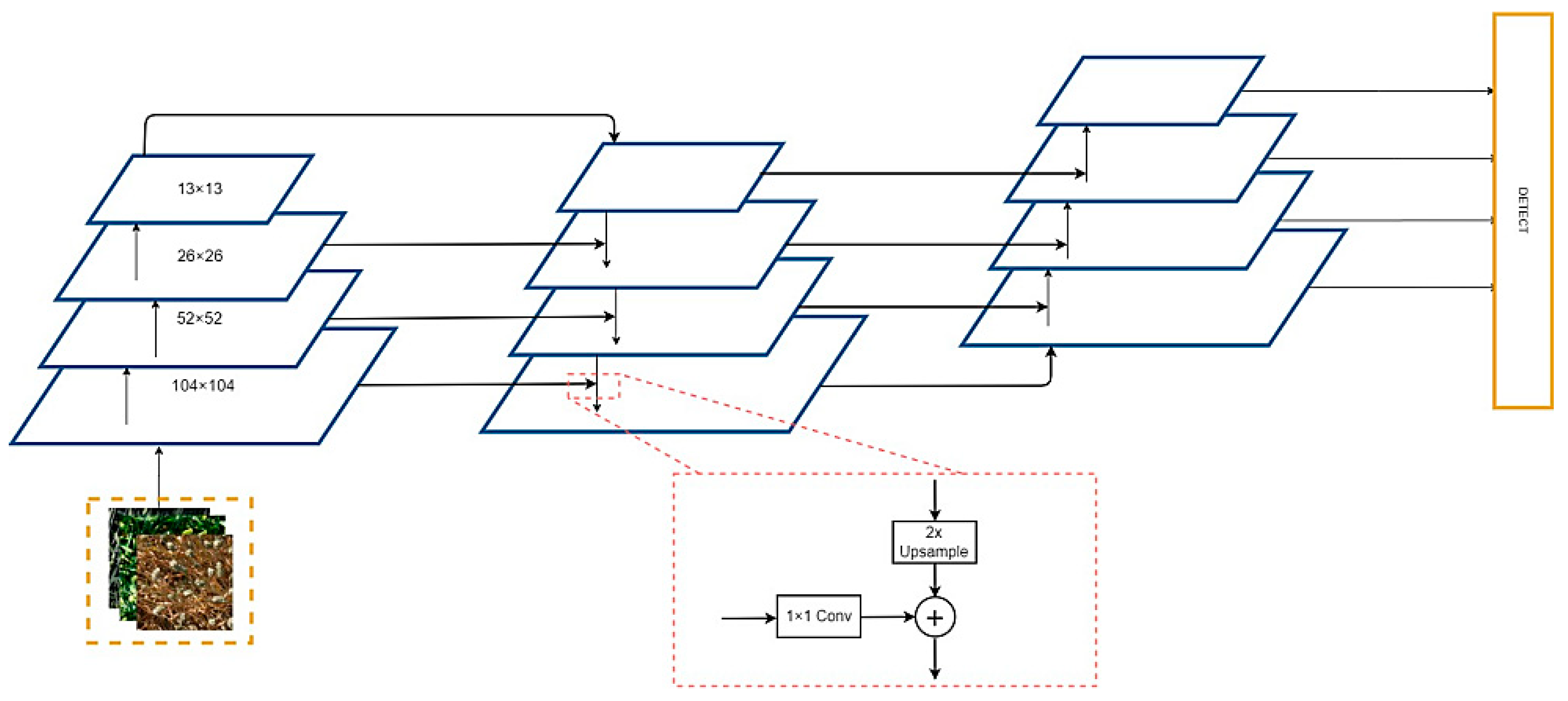
2.2.1. Feature Extractor
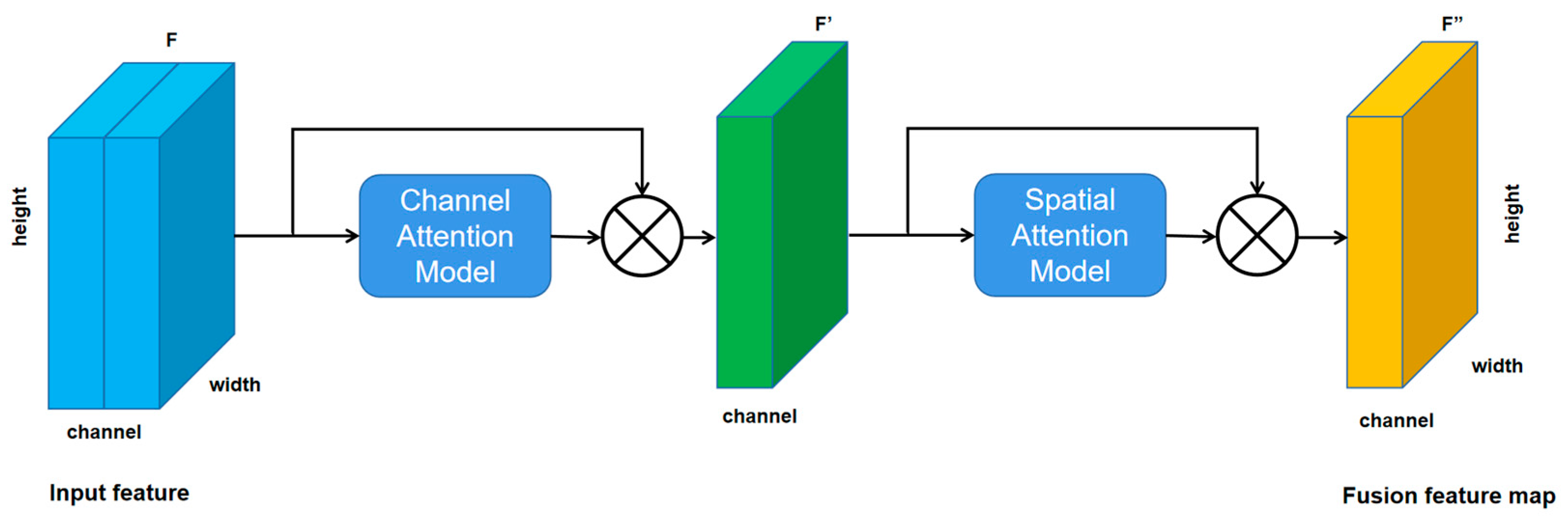
2.2.2. Introduce Convolutional Attention Module
2.2.3. Introduce Target Box Regression
2.2.4. Loss Function
2.3. An Improved Wheat Ear Detection Counting Model Based on YOLO v5
2.4. Evaluation of the Model Performance
3. Results
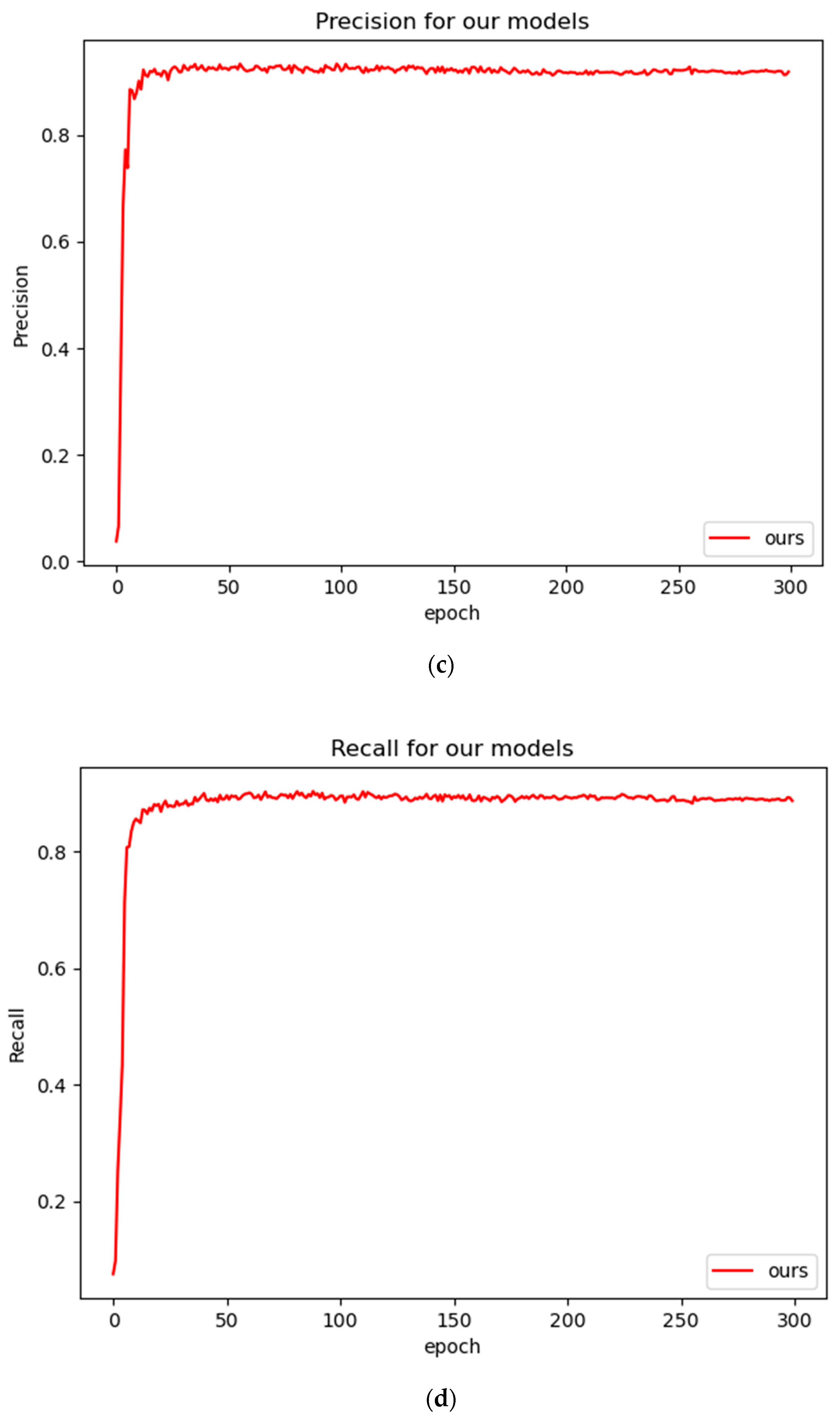
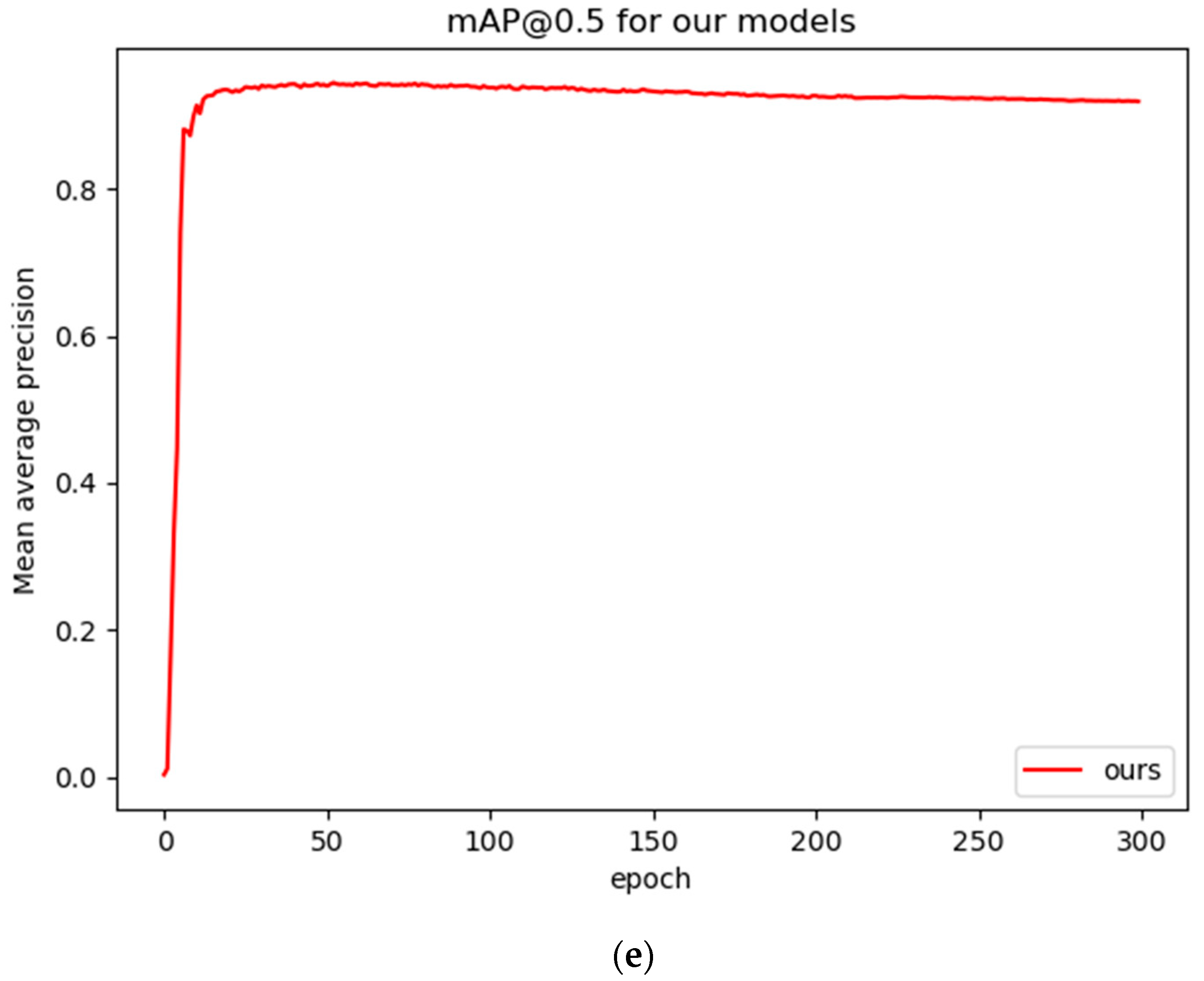
3.1. Model Training
3.2. Results of Detecting Wheat Ears
4. Discussion
Comparison of the Effect of Wheat Ear Detection and Counting under a Complex Background
5. Conclusions
Author Contributions
Funding
Acknowledgments
Conflicts of Interest
References
- Slafer, G.A.; Savin Sadras, V.O. Coarse and fine regulation of wheat yield components in response to genotype and environment. Field Crop. Res. 2014, 157, 71–83. [Google Scholar] [CrossRef]
- Ying, H.; Jian, W.; Mao, R.; Ying, S. Remote Sensing Model for Dynamic Prediction of Maize and Wheat Yield in the United States. J. Ecol. 2009, 28, 2142–2146. [Google Scholar]
- Xiu, Z.; Xiu, L.; Wen, Y.; Huai, Y. Annual prediction model of wheat yield in Rizhao city based on SPSS. China Agric. Bull. 2010, 26, 295–297. [Google Scholar]
- Liu, T.; Sun, C.M.; Wang, L.J.; Song, X.C.; Zhu, X.K.; Guo, W.S. Image processing technology-based counting of wheat ears in large fields. J. Agric. Mach. 2014, 45, 282–290. [Google Scholar]
- Du, Y.; Cai, Y.C.; Tan, C.W.; Li, Z.H.; Yang, G.J.; Feng, H.K.; Han, D. A method for counting the number of wheat spikes in the field based on super pixel segmentation. Chin. Agric. Sci. 2019, 52, 21–33. [Google Scholar]
- Li, Y.; Du, S.; Yao, M.; Yi, Y.; Yang, J.; Ding, Q.; He, R. Field wheat ear counting and yield prediction method based on wheat population images. J. Agric. Eng. 2018, 34, 193–202. [Google Scholar]
- Zhou, C.; Liang, D.; Yang, X.; Xu, B.; Yang, G. Recognition of Wheat Spike from Field Based Phenotype Platform Using Multi-Sensor Fusion and Improved Maximum Entropy Segmentation Algorithms. Remote Sens. 2018, 10, 246. [Google Scholar] [CrossRef] [Green Version]
- Li, Y.; Shiwei, D.; Min, Y.; Yingwu, Y.; Jianfeng, Y.; Qishuo, D.; Ruiyin, H. Method for wheatear counting and yield predicting based on image of wheatear population in field. Nongye Gongcheng Xuebao/Trans. Chin. Soc. Agric. Eng. 2018, 21, 185–194. [Google Scholar]
- Shrestha, B.L.; Kang, Y.M.; Yu, D.; Baik, O.D. A two-camera machine vision approach to separating and identifying laboratory sprouted wheat kernels. Biosyst. Eng. 2016, 147, 265–273. [Google Scholar] [CrossRef]
- Jose, A.F.; Lootens, P.; Irene, B.; Derycke, V.; Kefauver, S.C. Automatic wheat ear counting using machine learning based on RGB UAV imagery. Plant J. 2020, 103, 1603–1613. [Google Scholar]
- Xu, X.; Li, H.; Yin, F.; Xi, L.; Ma, X. Wheat ear counting using k-means clustering segmentation and convolutional neural network. Plant Methods 2020, 16, 106. [Google Scholar] [CrossRef] [PubMed]
- Girshick, R.; Donahue, J.; Darrell, T.; Malik, J. Rich feature hierarchies for accurate object detection and semantic segmentation. In Proceedings of the IEEE Conference on Computer Vision and Pattern Recognition, Columbus, OH, USA, 24–28 June 2014; pp. 580–587. [Google Scholar]
- Ren, S.; He, K.; Girshick, R.; Sun, J. Faster R-CNN: Towards Real-Time Object Detection with Region Proposal Networks. IEEE Trans. Pattern Anal. Mach. Intell. 2017, 39, 1137–1149. [Google Scholar] [CrossRef] [PubMed] [Green Version]
- Liu, W.; Anguelov, D.; Erhan, D.; Szegedy, C.; Reed, S.; Fu, C.-Y.; Berg, A.C. SSD: Single Shot MultiBox Detector; Springer: Cham, Switzerland, 2016. [Google Scholar]
- Hasan, M.M.; Chopin, J.P.; Laga, H.; Miklavcic, S.J. Detection and analysis of wheat spikes using Convolutional Neural Networks. Plant Methods 2018, 14, 1–13. [Google Scholar] [CrossRef] [PubMed] [Green Version]
- Madec, S.; Jin, X.; Lu, H.; De Solan, B.; Liu, S.; Duyme, F.; Baret, F. Ear density estimation from high resolution RGB imagery using deep learning technique. Agric. For. Meteorol. 2019, 264, 225–234. [Google Scholar] [CrossRef]
- Liang, X.; Chen, Q.; Dong, C.; Yang, C. Study on Maize Ear Detection Based on deep learning and unmanned aerial vehicle remote sensing technology. Fujian J. Agric. 2020, 35, 456–464. [Google Scholar]
- Xiong, H.; Cao, Z.; Lu, H.; Madec, S.; Shen, C. TasselNetv2: In-field counting of wheat spikes with context-augmented local regression networks. Plant Methods 2019, 15, 150. [Google Scholar] [CrossRef]
- Yao, J.; Qi, J.; Zhang, J.; Shao, H.; Yang, J.; Li, X. A Real-Time Detection Algorithm for Kiwifruit Defects Based on YOLOv5. Electronics 2021, 10, 1711. [Google Scholar] [CrossRef]
- Wang, D.; Fu, Y.; Yang, G.; Yang, X.; Zhang, D. Combined use of FCN and Harris corner detection for counting wheat ears in field conditions. IEEE Access 2019, 7, 178930–178941. [Google Scholar] [CrossRef]
- Sadeghi-Tehran, P.; Virlet, N.; Ampe, E.M.; Reyns, P.; Hawkesford, M.J. DeepCount: In-Field Automatic Quantification of Wheat Spikes Using Simple Linear Iterative Clustering and Deep Convolutional Neural Networks. Front. Plant Sci. 2019, 10, 1176. [Google Scholar] [CrossRef]
- Redmon, J.; Divvala, S.; Girshick, R.; Farhadi, A. You Only Look Once: Unified, Real-Time Object Detection. In Proceedings of the IEEE Conference on Computer Vision and Pattern Recognition (CVPR), Las Vegas, NV, USA, 27–30 June 2016. [Google Scholar]
- Redmon, J.; Farhadi, A. YOLO9000: Better, Faster, Stronger. In Proceedings of the IEEE Conference on Computer Vision and Pattern Recognition (CVPR), Honolulu, HI, USA, 21–26 July 2017; pp. 6517–6525. [Google Scholar]
- Redmon, J.; Farhadi, A. YOLOv3: An Incremental Improvement. arXiv 2018, arXiv:1804.02767. [Google Scholar]
- Bochkovskiy, A.; Wang, C.Y.; Liao, H.Y.M. Yolov4: Optimal speed and accuracy of object detection. arXiv 2020, arXiv:2004.10934. [Google Scholar]
- Woo, S.; Park, J.; Lee, J.; Kweon, I.S. CBAM: Convolutional block attention module. In Proceedings of the 2018 European Conference on Computer Vision (ECCV), Munich, Germany, 8–14 September 2018; p. 11211. [Google Scholar]
- Rezatofighi, H.; Tsoi, N.; Gwak, J.Y.; Sadeghian, A.; Reid, I.; Savarese, S. Generalized Intersection over Union: A Metric and A Loss for Bounding Box Regression. In Proceedings of the 2019 IEEE/CVF Conference on Computer Vision and Pattern Recognition (CVPR), Long Beach, CA, USA, 15–20 June 2019. [Google Scholar]
- David, E.; Madec, S.; Sadeghi-Tehran, P.; Aasen, H.; Zheng, B.; Liu, S.; Kirchgessner, N.; Ishikawa, G.; Nagasawa, K.; Badhon, M.A.; et al. Global wheat head detection (GWHD) dataset: A large and diverse dataset of high resolution RGB labelled images to develop and benchmark wheat head detection methods. Plant Phenomics 2020, 2020, 3521852. [Google Scholar] [CrossRef] [PubMed]
- Lin, T.Y.; Dollár, P.; Girshick, R.; He, K.; Hariharan, B.; Belongie, S. Feature Pyramid Networks for Object Detection. In Proceedings of the IEEE Conference on Computer Vision and Pattern Recognition (CVPR), Honolulu, HI, USA, 21–26 July 2017. [Google Scholar]
- Liu, S.; Qi, L.; Qin, H.; Shi, J.; Jia, J. Path Aggregation Network for Instance Segmentation. In Proceedings of the IEEE Conference on Computer Vision and Pattern Recognition, Salt Lake City, UT, USA, 18–23 June 2018. [Google Scholar]
- Neubeck, A.; Van Gool, L. Efficient non-maximum suppression. In Proceedings of the 18th International Conference on Pattern Recognition (ICPR’06), IEEE, Hong Kong, China, 20–24 August 2006; Volume 3, pp. 850–855. [Google Scholar]
- Wang, Y.; Zhang, Y.; Huang, L.; Zhao, F. Study on wheat ear target detection algorithm based on convolution neural network. Softw. Eng. 2021, 24, 6–10. [Google Scholar]
- Zhu, Y. Rapid Detection and Counting of Wheat Ears in the Field Using YOLOv4 with Attention Module. Agronomy 2021, 11, 1202. [Google Scholar]
- Oksuz, K.; Cam, B.C.; Kalkan, S.; Akbas, E. Imbalance Problems in Object Detection: A Review. IEEE Trans. Pattern Anal. Mach. Intell. 2020, 43, 3388–3415. [Google Scholar] [CrossRef] [PubMed] [Green Version]


| Title 1 | Image Number | Width | Height | Wheat Frame | Coordinates Source |
|---|---|---|---|---|---|
| 0 | b6ab77fd7 | 1024 | 1024 | [834.0, 222.0, 56.0, 360] | usask_l |
| 1 | b6ab77fd7 | 1024 | 1024 | [226.0, 548.0, 130.0, 580] | usask_l |
| 2 | b6ab77fd7 | 1024 | 1024 | [377.0, 504.0, 74.0, 160.0] | usask_l |
| 3 | b6ab77fd7 | 1024 | 1024 | [834.0, 95.0, 109.0, 107.0] | usask_l |
| Characteristic Map Size | Characteristic Map Size | ||
|---|---|---|---|
| 13 × 13 | [116, 90] | [156, 198] | [373, 326] |
| 26 × 26 | [30, 61] | [62, 45] | [59, 119] |
| 52 × 52 | [10, 13] | [16, 30] | [33, 23] |
| 104 × 104 | [5, 6] | [8, 14] | [15, 11] |
| Data | F1-Score/% | Precision | Recall | mAP |
|---|---|---|---|---|
| GWHDD | 89.3% | 88.5% | 98.0% | 94.3% |
| Model | Precision | Recall | mAP (%) |
|---|---|---|---|
| Faster-RCNN | 47.5% | 46.9% | 39.2% |
| SSD | 91.2% | 36.7% | 69.5% |
| YOLO v3 | 76.6% | 92.2% | 88.8% |
| Reference [32] | 76.9% | 93.1% | 89.5% |
| YOLO v4 | 77.8% | 93.4% | 90.3% |
| Reference [33] | 87.5% | 91.0% | 93.1% |
| YOLO v5 | 88.7% | 98.0% | 91.9% |
| Our method | 88.5% | 98.0% | 94.3% |
| Test Set | Precision | Recall | F1-Score | mAP (%) |
|---|---|---|---|---|
| A | 0.941 | 0.936 | 0.941 | 97.2% |
| B | 0.948 | 0.902 | 0.923 | 95.8% |
| A + B | 0.955 | 0.910 | 0.932 | 96.7% |
| Model | Precision | Recall | mAP (%) |
|---|---|---|---|
| YOLO v5 | 88.70% | 98.01% | 91.60% |
| YOLO v5 + 4× | 89.63% | 98.04% | 94.13% |
| YOLO v5 + 4× + CBAM | 88.52% | 98.06% | 94.32% |
Publisher’s Note: MDPI stays neutral with regard to jurisdictional claims in published maps and institutional affiliations. |
© 2022 by the authors. Licensee MDPI, Basel, Switzerland. This article is an open access article distributed under the terms and conditions of the Creative Commons Attribution (CC BY) license (https://creativecommons.org/licenses/by/4.0/).
Share and Cite
Li, R.; Wu, Y. Improved YOLO v5 Wheat Ear Detection Algorithm Based on Attention Mechanism. Electronics 2022, 11, 1673. https://doi.org/10.3390/electronics11111673
Li R, Wu Y. Improved YOLO v5 Wheat Ear Detection Algorithm Based on Attention Mechanism. Electronics. 2022; 11(11):1673. https://doi.org/10.3390/electronics11111673
Chicago/Turabian StyleLi, Rui, and Yanpeng Wu. 2022. "Improved YOLO v5 Wheat Ear Detection Algorithm Based on Attention Mechanism" Electronics 11, no. 11: 1673. https://doi.org/10.3390/electronics11111673
APA StyleLi, R., & Wu, Y. (2022). Improved YOLO v5 Wheat Ear Detection Algorithm Based on Attention Mechanism. Electronics, 11(11), 1673. https://doi.org/10.3390/electronics11111673