Article

Monoscopic Phase Measuring Deflectometry Simulation and Verification

1
Shanghai Institute of Technical Physics, Chinese Academy of Sciences, Shanghai 200083, China
2
School of Information Science and Technology, ShanghaiTech University, Shanghai 201210, China
3
School of Electronic, Electrical and Communication Engineering, University of Chinese Academy of Sciences, Beijing 100049, China
*
Authors to whom correspondence should be addressed.
Electronics 2022, 11(10), 1634; https://doi.org/10.3390/electronics11101634
Submission received: 19 April 2022 / Revised: 14 May 2022 / Accepted: 16 May 2022 / Published: 20 May 2022
(This article belongs to the Special Issue Deep Perception in Autonomous Driving)

Abstract

:
The three-dimensional (3D) shape of specular surfaces is important in aerospace, precision instrumentation, and automotive manufacturing. The phase measuring deflectometry (PMD) method is an efficient and highly accurate technique to measure specular surfaces. A novel simulation model with simulated fringe patterns for monoscopic PMD is developed in this study. Based on the pre-calibration and the ray-tracing model of the monoscopic PMD system, a comprehensive model from deformed pattern generation to shape reconstruction was constructed. Experimental results showed that this model achieved high levels of measuring accuracy in both planar and concave surfaces measurement. In planar surface measurement, the peak to valley (PV) value and root mean square (RMS) value of the reconstructed shape can reach 26.93 nm and 10.32 nm, respectively. In addition, the accuracy of the reconstructed concave surface can reach a micrometre scale. This work potentially fills critical gaps in monoscopic PMD simulation and provides a cost-effective method of PMD study.

1. Introduction

The precise three-dimensional (3D) shape measurement of free-form specular surfaces is important for a wide range of applications in space observatory, scientific research, optical precision measurement, and automotive manufacturing [1,2,3,4,5]. The 3D shape measurement of specular surfaces is not implemented in the same way as diffuse reflection surfaces measurement due to their reflecting properties. Generally, there are two competitive method categories for specular surface measurement [6,7], which are interferometry [8] and deflectometry [9,10,11,12,13,14]. Extensive studies [12,13,14] suggest that deflectometry methods such as phase measuring deflectometry (PMD) can achieve the same accuracy with a full-field measuring range. Moreover, it has many advantages of large dynamic range, noncontact operation, and high precision [10,15]. PMD typically displays sinusoidal fringe patterns on screens and captures the deformed reflected patterns through a camera or multiple cameras. Phase information is then extracted from the deformed patterns, and 3D shapes of test surfaces can be reconstructed [13]. The PMD method has become an important aspect of specular surface shape measurement.
The modelling of the measuring system plays a critical role in developing PMD methods. Recent work has shown that PMD models can simulate the ideal condition and help improve the performance of the measuring system. Zhao et al. [16] carried out a virtual direct phase measuring deflectometry (DPMD) system by combining DPMD and a pinhole imaging model, aiming to optimize the parameters of the measurement system and evaluate the performance in DPMD applications. The high-accuracy 3D shape of specular objects with discontinuous surfaces was obtained from the optimized system. Huang et al. [17] proposed modal phase measuring deflectometry to simultaneously estimate the height and slopes of test surfaces in PMD. Its feasibility was demonstrated in simulations of monoscopic PMD and stereo-PMD systems. Simulation models can be separated from actual measuring systems and implemented independently, especially when the experimental condition is limited. In addition, simulation models exploit precise mathematic models to deepen the understanding of PMD methods and provide a new direction to prompt deflectometry method research.
In monoscopic phase measuring deflectometry (MPMD), the deformed fringe patterns carry the shape information of the test surface. They are captured by one camera and then analyzed by the measuring system to reconstruct the 3D shape of surfaces [18,19]. The fringe patterns are critical factors of MPMD, and the simulation of deformed fringe patterns should also be studied in the MPMD simulation model. However, deformed fringe patterns are both shape-specific and system-specific [6,18,20]. In other words, the generation of fringe patterns is not independent of the actual measuring system and the specific surface being tested. The simulation of deformed fringe patterns needs to combine system configurations and surface situations in the traditional measuring process, which increases the simulating difficulty. Recent studies mainly focused on the mathematical models of specular surfaces but rarely considered the process of fringe generation.
This work proposes a new simulated monoscopic phase measuring deflectometry (SMPMD) model that can simulate the steps from surface-tested deformed fringe generation to shape reconstruction. Different from the traditional calibration, all the system parameters of this simulation model are entirely acquired through the camera calibration process, which involves no measuring parameters of distance and angles. Moreover, a model based on system parameters and a ray-tracing model was established to simulate the deformed patterns. A planar specular surface and concave mirror model were built and tested to evaluate the performance of the model. The paper has been organized in the following way. Section 2 explains the basic principle of the SMPMD model, Section 3 shows the experimental results of pattern simulation and the performance of the SMPMD model, and Section 4 concludes this work.

2. Principle of the SMPMD Model

The SMPMD model consists of two parts: the simulated pattern generation (SPG) model and the MPMD measuring model. The SPG model simulates the deformed pattern sampling process and generates patterns based on tested surfaces. The MPMD measuring model is based on the MPMD method [13], which contains image preprocessing, phase-shifting technique, phase unwrapping, gradient calculation, and integral shape reconstruction. The latter model focuses on the 3D reconstruction from generated fringe patterns.

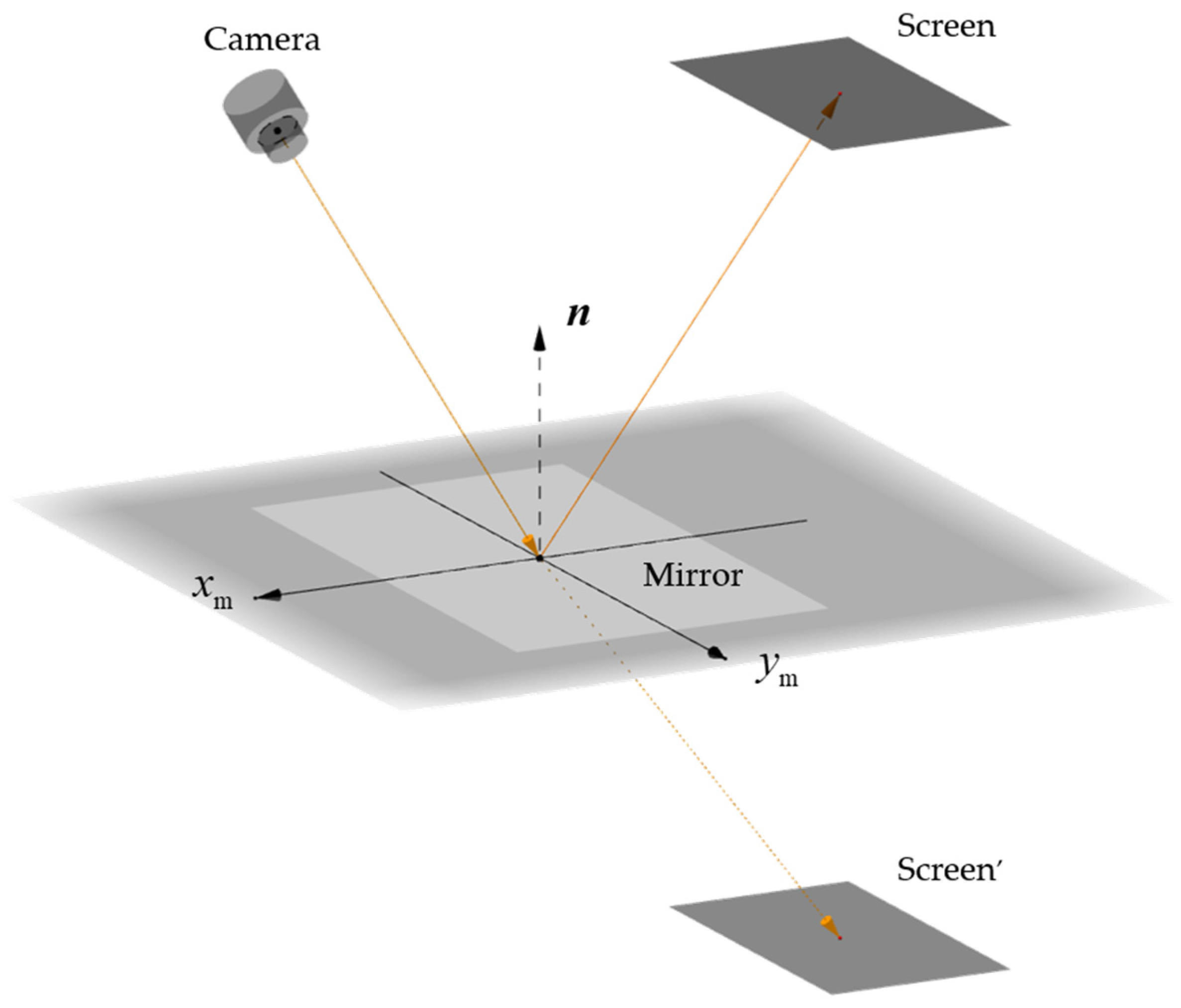
2.1. The Principle of the SPG Model

To build a pattern-generation model of the MPMD system, a general setup of the MPMD system is utilized as a reference, which is demonstrated in Figure 1. The system consists of an LCD screen as a light source, a camera with a lens as the measuring sensor, and a computing device as the postprocessing unit. The measuring system is established in a proper configuration by a precise system calibration so that patterns deformed by the tested surface can be captured correctly by the camera. The sum of normalized direction vectors of incident light from screen pixels and corresponding reflected light to the camera determines the normal vectors of surface points through the reflection law.
Coordinate transformations are necessary for this work to construct the SPG model. There are four physical coordinate systems introduced in this measuring system model, which are demonstrated in Figure 2. They include the Screen Coordinate System (SCS), View Coordinate System (VCS), Camera Coordinate System (CCS), and Mirror Coordinate System (MCS). In this work, the World Coordinate System (WCS) is MCS, and VCS is the mirror coordinate system of SCS. Both the coordinate transformation between MCS and CCS and the coordinate transformation between VCS and CCS are determined by an improved camera calibration [21]. The camera calibration requires the camera to observe a planar checkboard from a few different orientations. To figure out the transformation between MCS and CCS, a planar checkboard is placed on the reference mirror plane, and the image of the checkboard is captured. A virtual planar checkboard image that is the same as the planar checkboard is displayed on the screen, and a flat mirror without markers is introduced to establish the relation between VCS and CCS. Note that the lens is fixed when the camera is calibrated. A camera-calibration algorithm is then introduced to estimate the camera parameters. The camera parameters involve intrinsic parameters, distortion coefficients, and extrinsic parameters. The rotation matrices and translation vectors among coordinate systems are involved in the extrinsic parameters. The transformation relation between SCS and CCS can be built by the mirroring relationship between VCS and SCS, and it can be denoted as
{ R s = ( I 2 R m e e T R m T ) R v T s = ( I 2 R m e e T R m T ) T v + 2 R m e e T R m T T m ,
where R s is the rotation matrix from SCS to CCS, T s is the translation vector from SCS to CCS, R m and T m are the rotation matrix and translation vector from MCS to CCS, R v and T v is the rotation matrix and translation vector from the View Coordinate System (VCS) to CCS, and I is a 3   ×   3 unit matrix and vector e = [0 0 1]T.
The direction of the optical path can be analyzed reversely in the MPMD system. Following the conventional camera calibration model [21], the camera light ray is considered as a probe ray, and for a camera pixel c p : ( u cp , v cp , 1 ) T , the corresponding point P :   ( x c , y c , z c ) T of the light from the camera in CCS can be calculated by
s [ u cp v cp 1 ]   =   K [ R | T ] [ x c y c z c 1 ] ,
where s is a scaling factor, K is the intrinsic matrix, and R and T are the extrinsic matrix and translation vector. These parameters are obtained by camera calibration. Directional vectors of camera pixels can then be calculated by projection points and the light source of the camera, the origin of CCS.
When a test surface is installed on the reference plane with a known pose and shape, a light ray from a camera pixel hits the specular surface at M: ( x m , y m , z m ) T and then is reflected. The reflected light directional vector r : ( m r , n r , p r ) T can be obtained by
r = 2 n × ( n · i ) i ,
where n is the normalized normal vector at point M on the test surface, and i is the normalized directional vector of the incident ray, which denotes the dot product of vectors. The reflected ray equations can be determined by vector r and point M.
The intersection of the reflected ray and the screen surface can be obtained from the screen surface equation and light ray equation. For the screen surface equation, it is the xOy plane in Screen Coordinate System (SCS), and the normal vector and coordinate of a point on the plane can be transformed into the Mirror Coordinate System (MCS) by R s and T s . The normal vector n s and the point coordinate P s of the equation can be determined by:
{ n s = R s e P s = T s ,
and finally hits the screen at the point S : ( x s , y s , z s ) T , which can be calculated by:
[ x s y s z s ] = ( R s e ) T ( M T s ) 2 ( R s e ) T ( n   ×   ( n · i ) i ) · [ m r n r p r ] + [ x m y m z m ] .
Note that point S now is denoted in WCS, and transformation from WCS to the Screen Pixel Coordinate System (SPCS) is required to calculate the screen pixel coordinate on the screen. Since the virtual mirroring point S : ( x s , y s , z s ) T of point S is on the xOy plane in VCS, this transformation can be built in two steps: a transformation from WCS to VCS and a transformation from VCS to SPCS. The former transformation contains transformations from WCS to CCS and from CCS to VCS, so the coordinate V: ( x v , y v , z v ) T of point S′ in VCS can be calculated by
[ x v y v z v ] = R v 1 ( R m [ x s y s z s ] + T m T v ) .
The latter transformation from VCS to SPCS contains transformations from VCS to the View Pixel Coordinate System (VPCS) and from VPCS to SPCS. It can be determined by
[ u v v v 1 ] = i n s v · [ x v y v z v ] ,
where i n s v = [ 1 / f x 0 O x 0 1 / f y O y 0 0 1 ] is a transformation associated with the screen intrinsic parameters, which converts the view coordinate into the view pixel coordinate. Factors f x and f y are the height and width of the screen pixel, respectively, and ( O x , O y ) is the view pixel coordinate of the VCS origin.
As the correspondence between camera pixels and screen pixels is established, the grey value of each camera pixel is the corresponding screen pixel’s grayscale. As a result, simulated pattern images can be generated as long as the displayed fringe patterns on the screen are known. In this work, a three-step phase-shifting method is applied. The grey intensity of screen pixels can be calculated as
{ I ( x , y ) = I 0 +   Acos ( 2 π x p x + 2 n π 3 ) I ( x , y ) = I 0 +   Acos ( 2 π y p y + 2 n π 3 ) ,
where n   =   0 , 1 , 2 , I 0 is the background intensity, A is the grey amplitude, p x and p y are the fringe periods in x and y directions. The grey intensity of each camera pixel can then be determined.

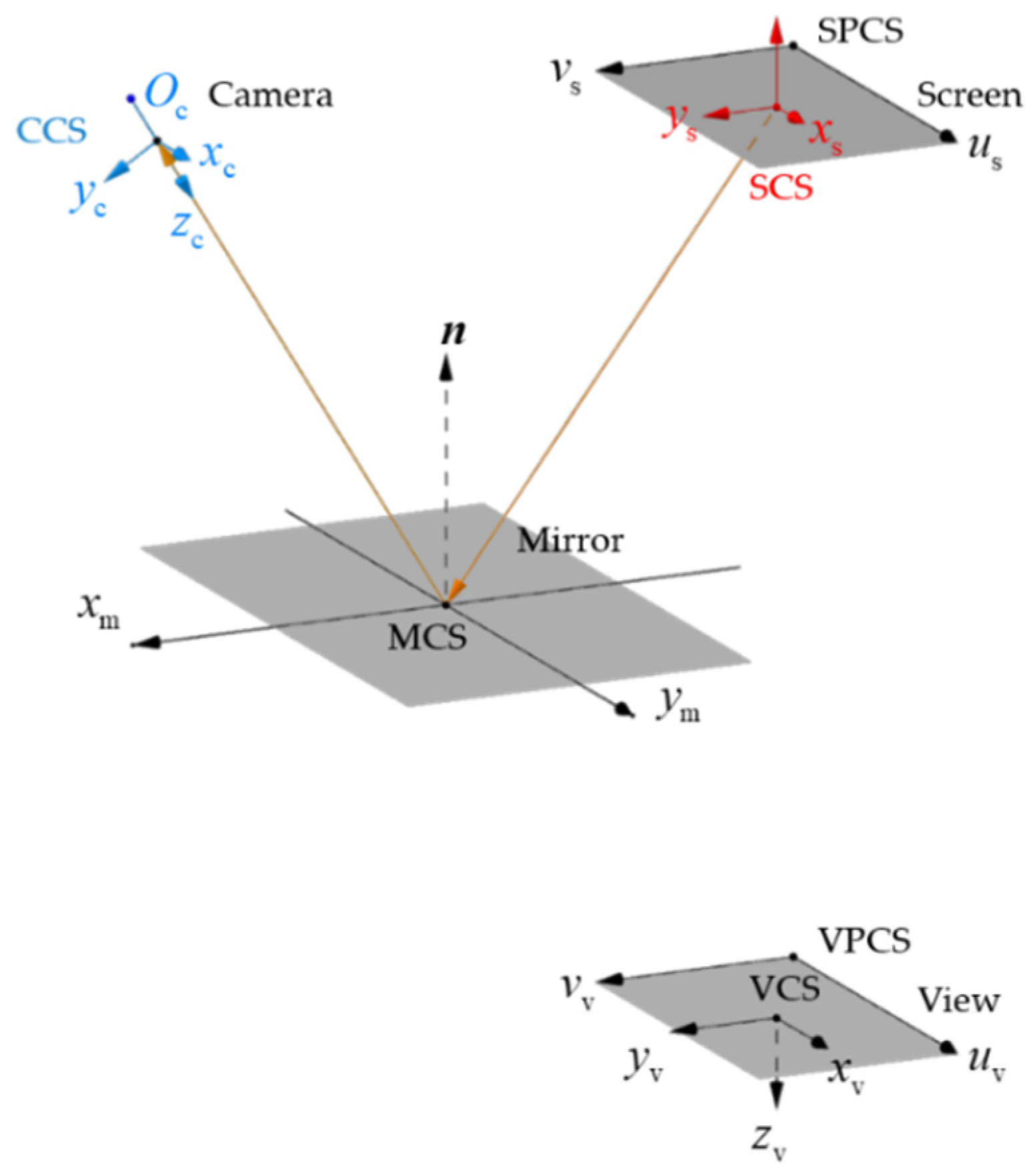
2.2. The Principle of the Simulated MPMD Model
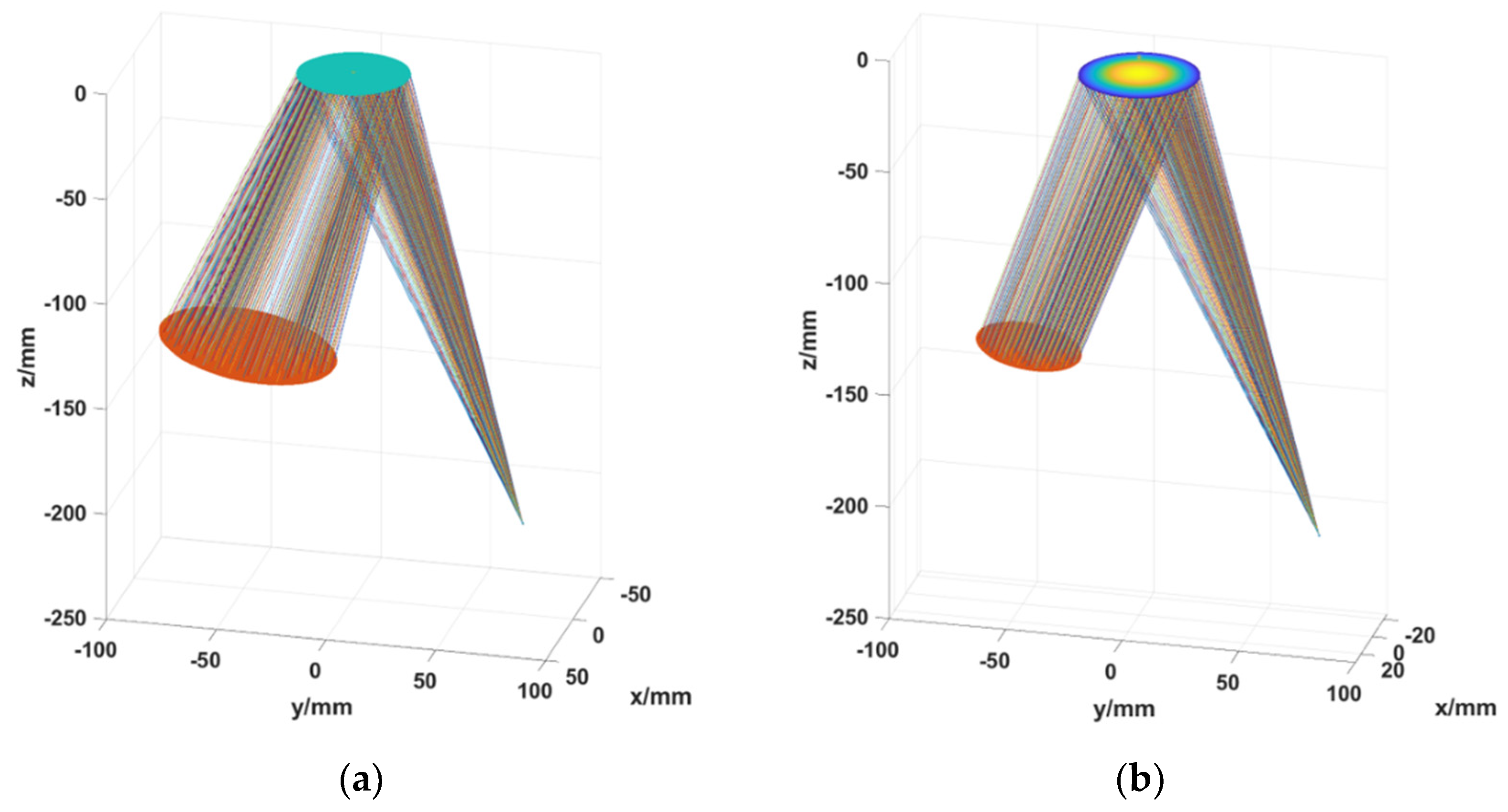
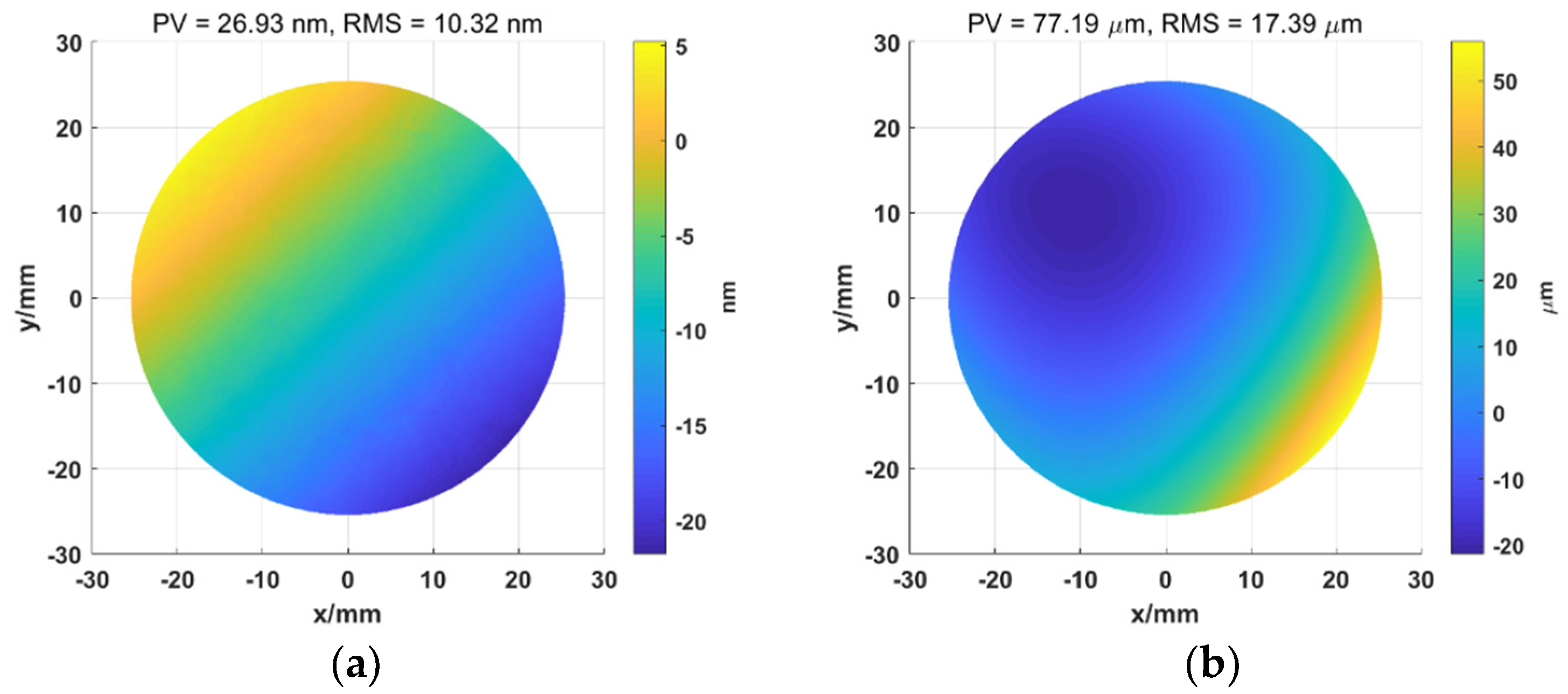
The key to the shape reconstruction model is to determine the correspondence among mirror, camera pixel, and screen pixel. As a traditional camera can be regarded as a probe ray model, every pair of the mirror pixel and the screen pixel corresponds to the same point in the camera model, the origin in CCS. Therefore, the correspondence between the mirror pixel and screen pixel determines the gradient of the reconstructed shape. To build this correspondence, as mentioned, a three-step phase-shifting method is applied in this work, and phase maps in two directions are then retrieved and unwrapped [22]. Screen pixel coordinates corresponding to camera pixels and their positions in MCS can be determined. Note that the step of image undistorting is not involved in the model to simplify the complexity of the simulation. Regarding MCS coordinates of reference specular surface as initial coordinates of measured surface, normal vectors of mirror pixels can be calculated by
n =   ( i + r ) ,
where i and r are the normalized directional vectors of the incident ray and the reflected ray. Gradient data of each mirror pixel can be available from the corresponding normal vectors [12]. The height of the tested surface is then can be calculated with the zonal integration method [23].

3. Results

Experiments are carried out to test the performance of the SMPMD model. As shown in Figure 3, the SMPMD model is established. System parameters of this model are obtained from a typical calibration of an MPMD measuring system that consists of an LCD screen with a resolution of 1080 × 1920 pixels and a high-speed camera with a 16 mm lens that has a resolution of 2048 × 2048 pixels at a frame rate of 30 frames per second. System calibration, including geometric relationship calibration, is implemented in the camera calibration. To decrease the effects of lens distortion on the model, camera calibration [21] was first implemented to estimate the camera parameters of the lens and image sensor. Camera parameters include intrinsic parameters, extrinsic parameters, and distortion coefficients. Extrinsic parameters, distortion coefficient, the undistortImage function in the Matlab toolbox, and the checkboard images in calibration are applied to further recalibrate rotation matrices and translation vectors among coordinate systems. A typical planar specular surface mathematic model and a typical concave mirror model based on a real concave mirror are constructed and utilized for testing the performance of the model. It should be noted that the centerlines of the models are through the origin of the mirror coordinate system. Their diameters are equally 50.8 mm. For the concave mirror, its focus is 200 mm, and its height from the reference plane is 8 mm. The shapes of mirror models are shown in Figure 4.
Taking the step-three phase-shifting method as a fringe pattern generating example, the initial phase of three images are 0 , 2 π / 3 , 4 π / 3 , respectively. Every period of fringe patterns contains eight screen pixels. The expression of fringe patterns can be denoted as
{ I ( x , y ) =   0.5 + 0.5 cos ( π x 8 + 2 n π 3 ) , n =   0 , 1 , 2 I ( x , y ) =   0.5 + 0.5 cos ( π y 8 + 2 n π 3 ) , n =   0 , 1 , 2
One of the generated sinusoidal fringe patterns for planar mirror and concave mirror is shown in Figure 5, respectively. Totally, there are three images in horizontal and vertical directions for one mirror measurement, respectively. Images are generated in the camera view, and the resolution is 2048 × 2048 pixels.
The shape reconstruction of simulated mirrors is completed via the phase-shifting method, phase unwrapping, gradient calculation, and shape reconstruction. The reconstructed profile is shown in Figure 6. For the planar mirror, the peak to valley (PV) value of the reconstructed shape is about 26.93 nm, and the root mean square (RMS) value is 10.32 nm. For the concave mirror, the PV value is 812.80 μm, and the RMS value is 465.22 μm. It can be found that the simulated fringe patterns can be utilized for reconstructing the shape of the specular surface under test, and the error is on a nanometer scale. For concave mirror sensing, the reconstructed shape of the concave surface is nearly identical to the mathematical model, and the error of the PV value is about 7 μm. The overall shape of the concave mirror can be recovered through the SMPMD model.
The residual maps between mathematic models and reconstructed shapes of mirrors are shown in Figure 7. As the reference shape of the planar mirror is the xOy plane in MCS, the residual map is the same as the reconstructed planar mirror’s shape. For the concave mirror, the mean error is 0.32 μm, and the RMS value of error is 17.39 μm.
Experiments showed that the system error of planar surface measurement was mainly from the error of coordinates in VPCS in generating the deformed fringe patterns. The mean error between reference pixel coordinates obtained in pattern generation and the calculated pixel coordinates by the phase-shifting method was 4.04 × 10 4 pixels in the x direction and 5.24 × 10 4 pixels in the y direction. When the reference pixel coordinates were substituted into the simulation model, the PV value decreased dramatically to 5.06 × 10 15 nm, and the RMS value decreased dramatically to 3.05 × 10 15 nm. For concave surfaces, the system error of concave surface measurement is relatively complicated. A similar experiment was conducted in concave model measurement: the decrease in the PV value in the residual map was 0.08 μm, and the decrease in the RMS value in the residual map was 0.03 μm. The simulated fringe patterns are effective and can be utilized for reconstructing the shape of both planar and concave specular surfaces. The MPMD model can simulate the entire measuring process and achieve a high measurement accuracy.

4. Conclusions

A novel simulation model has been developed based on the monoscopic phase measuring deflectometry (MPMD) method. Simulated fringe patterns of both a planar surface and concave surface were generated. The performance of the SMPMD model was evaluated by two types of specular surface shape measurement. The reconstructed shape PV value from simulated fringe patterns of planar specular surface can reach 26.93 nm, and the RMS value can reach 10.32 nm, achieving a high level of modelling accuracy. The accuracy of the reconstructed concave surface can also reach a micrometre scale. Our study has been one of the first attempts to establish a mathematical model of the MPMD measuring process to provide a cost-effective and universal method for MPMD, further research, and fill key gaps in terms of MPMD simulation. Future research could be focused on complicated specular surface sensing with this simulation model.

Author Contributions

Conceptualization, Z.L., D.Y., Q.Z. and H.G.; methodology, Z.L., D.Y., Q.Z. and H.G.; software, Z.L.; validation, Z.L.; formal analysis, Z.L.; investigation, Z.L.; resources, D.Y. and Q.Z.; data curation, Z.L.; writing—original draft preparation, Z.L.; writing—review and editing, D.Y. and H.G.; visualization, Z.L.; supervision, D.Y. and H.G.; project administration, D.Y.; funding acquisition, D.Y.. All authors have read and agreed to the published version of the manuscript.

Funding

This research was funded by the National Natural Science Foundation of China (NSFC), grant number 12103075.

Institutional Review Board Statement

Not applicable.

Informed Consent Statement

Not applicable.

Data Availability Statement

Not applicable.

Conflicts of Interest

The authors declare no conflict of interest.

References

  1. Tang, T.; Deng, C.; Yang, T.; Zhong, D.; Ren, G.; Huang, Y.; Fu, C. Error-Based Observer of a Charge Couple Device Tracking Loop for Fast Steering Mirror. Sensors 2017, 17, 479. [Google Scholar] [CrossRef] [PubMed] [Green Version]
  2. Saif, B.; Chaney, D.; Greenfield, P.; Bluth, M.; Van Gorkom, K.; Smith, K.; Bluth, J.; Feinberg, L.; Wyant, J.C.; North-Morris, M.; et al. Measurement of picometer-scale mirror dynamics. Appl. Opt. 2017, 56, 6457–6465. [Google Scholar] [CrossRef] [PubMed]
  3. Coyle, L.; Chonis, T.; Smith, K.; Knight, J.S.; Acton, D.S.; Howard, J.; Feinberg, L. Optical Assessment of the James Webb Space Telescope Primary and Secondary Mirror Cryogenic Alignment with a Hartmann Test; SPIE: Bellingham, WA, USA, 2018; Volume 10706. [Google Scholar]
  4. Wang, W.; Sun, G.; Van Gool, L. Looking Beyond Single Images for Weakly Supervised Semantic Segmentation Learning. IEEE Trans. Pattern Anal. 2022. [Google Scholar] [CrossRef] [PubMed]
  5. Wang, W.; Zhou, T.; Porikli, F.; Crandall, D.; Van Gool, L. A survey on deep learning technique for video segmentation. arXiv 2021, arXiv:2107.01153. [Google Scholar]
  6. Xu, Y.; Gao, F.; Jiang, X. A brief review of the technological advancements of phase measuring deflectometry. PhotoniX 2020, 1, 14. [Google Scholar] [CrossRef]
  7. Schmit, J.; Faber, C.; Olesch, E.; Krobot, R.; Häusler, G.; Creath, K.; Towers, C.E.; Burke, J. Deflectometry challenges interferometry: The competition gets tougher! In Proceedings of the Interferometry XVI: Techniques and Analysis, San Diego, CA, USA, 12 August 2012. [Google Scholar]
  8. Xue, S.; Chen, S.; Tie, G. Near-null interferometry using an aspheric null lens generating a broad range of variable spherical aberration for flexible test of aspheres. Opt. Express 2018, 26, 31172–31189. [Google Scholar] [CrossRef] [PubMed]
  9. Wang, Y.M.; Xu, Y.J.; Zhang, Z.H.; Gao, F.; Jiang, X.Q. 3D Measurement of Structured Specular Surfaces Using Stereo Direct Phase Measurement Deflectometry. Machines 2021, 9, 170. [Google Scholar] [CrossRef]
  10. Zhang, Z.; Wang, Y.; Huang, S.; Liu, Y.; Chang, C.; Gao, F.; Jiang, X. Three-Dimensional Shape Measurements of Specular Objects Using Phase-Measuring Deflectometry. Sensors 2017, 17, 2835. [Google Scholar] [CrossRef] [PubMed] [Green Version]
  11. Liu, Y.; Huang, S.; Zhang, Z.; Gao, N.; Gao, F.; Jiang, X. Full-field 3D shape measurement of discontinuous specular objects by direct phase measuring deflectometry. Sci. Rep. 2017, 7, 10293. [Google Scholar] [CrossRef] [PubMed]
  12. Huang, L.; Ng, C.S.; Asundi, A.K. Dynamic three-dimensional sensing for specular surface with monoscopic fringe reflectometry. Opt. Express 2011, 19, 12809–12814. [Google Scholar] [CrossRef] [PubMed]
  13. Knauer, M.C.; Kaminski, J.; Hausler, G. Phase Measuring Deflectometry: A new approach to measure specular free-form surfaces. Opt. Metrol. Prod. Eng. 2004, 5457, 366–376. [Google Scholar] [CrossRef]
  14. Tang, Y.; Su, X.; Liu, Y.; Jing, H. 3D shape measurement of the aspheric mirror by advanced phase measuring deflectometry. Opt. Express 2008, 16, 15090–15096. [Google Scholar] [CrossRef] [PubMed]
  15. Zhang, Z.; Chang, C.; Liu, X.; Li, Z.; Shi, Y.; Gao, N.; Meng, Z. Phase measuring deflectometry for obtaining 3D shape of specular surface: A review of the state-of-the-art. Opt. Eng. 2021, 60, 020903. [Google Scholar] [CrossRef]
  16. Zhao, P.; Gao, N.; Zhang, Z.H.; Gao, F.; Jiang, X.Q. Performance analysis and evaluation of direct phase measuring deflectometry. Opt. Laser Eng. 2018, 103, 24–33. [Google Scholar] [CrossRef] [Green Version]
  17. Huang, L.; Xue, J.P.; Gao, B.; McPherson, C.; Beverage, J.; Idir, M. Modal phase measuring deflectometry. Opt. Express 2016, 24, 24649–24664. [Google Scholar] [CrossRef] [PubMed]
  18. Han, H.; Wu, S.; Song, Z.; Zhao, J. An Accurate Phase Measuring Deflectometry Method for 3D Reconstruction of Mirror-Like Specular Surface. In Proceedings of the 2019 2nd International Conference on Intelligent Autonomous Systems (ICoIAS), Singapore, 28 February–2 March 2019; pp. 20–24. [Google Scholar]
  19. Xu, Y.J.; Gao, F.; Jiang, X.Q. Enhancement of measurement accuracy of optical stereo deflectometry based on imaging model analysis. Opt. Laser Eng. 2018, 111, 1–7. [Google Scholar] [CrossRef]
  20. Zhang, X.; Li, D.; Wang, R.; Tang, H.; Luo, P.; Xu, K. Speckle pattern shifting deflectometry based on digital image correlation. Opt. Express 2019, 27, 25395–25409. [Google Scholar] [CrossRef] [PubMed]
  21. Zhang, Z.Y. A flexible new technique for camera calibration. IEEE Trans. Pattern Anal. 2000, 22, 1330–1334. [Google Scholar] [CrossRef] [Green Version]
  22. Herraez, M.A.; Burton, D.R.; Lalor, M.J.; Gdeisat, M.A. Fast two-dimensional phase-unwrapping algorithm based on sorting by reliability following a noncontinuous path. Appl. Opt. 2002, 41, 7437–7444. [Google Scholar] [CrossRef] [PubMed]
  23. Huang, L.; Xue, J.; Gao, B.; Zuo, C.; Idir, M. Zonal wavefront reconstruction in quadrilateral geometry for phase measuring deflectometry. Appl. Opt. 2017, 56, 5139–5144. [Google Scholar] [CrossRef] [PubMed]
Figure 1. The schematic diagram of monoscopic phase measuring deflectometry.
Electronics 11 01634 g001
Figure 2. The distributions of the coordinate systems in the MPMD measuring system.
Electronics 11 01634 g002
Figure 3. The simulation model of the SMPMD system. (a) The monoscopic deflectometric simulation model of the planar mirror. (b) The monoscopic deflectometric simulation model of the concave mirror. The configuration of the measuring system is the same as that of the planar mirror.
Electronics 11 01634 g003
Figure 4. The simulation shape of specular objects. (a) The planar mirror model, a 50.8 mm cylinder with reflecting surface on the xOy plane of MCS. (b) The concave mirror model with 50.8 mm diameters, its focus f = 200 mm, the height of the edge is 8 mm, and its shape is a concave mirror.
Electronics 11 01634 g004
Figure 5. One of the simulated fringe patterns in camera view for planar mirror and concave mirror. (a) The deformed horizontal fringe pattern image simulated for planar mirror. The resolution is 2048 × 2048 pixels; the sinusoidal fringe initial phase is 0, and the period is 8 screen pixels. (b) The deformed horizontal fringe pattern simulated for the 200 mm-focus concave mirror; its initial phase is 0, and the period of fringe patterns is 8 pixels.
Electronics 11 01634 g005
Figure 6. The reconstructed shape of specular objects through SPMD model. (a) The planar mirror with PV = 26.93 nm, RMS = 10.32 nm. (b) The concave mirror shape from reconstruction. PV = 812.80 μm, RMS = 465.22 μm.
Electronics 11 01634 g006
Figure 7. The residual map between the reference model and the reconstructed model of mirrors. (a) The residual map of the planar mirror; the RMS of error is 10.32 nm. (b) The residual map of the concave mirror; the RMS value of error is 17.39 μm.
Electronics 11 01634 g007
Publisher’s Note: MDPI stays neutral with regard to jurisdictional claims in published maps and institutional affiliations.

