
High-Speed Reservoir Computing Based on Circular-Side Hexagonal Resonator Microlaser with Optical Feedback

 ,
, 
Abstract
:1. Introduction
2. System Model and Methods
2.1. Theory
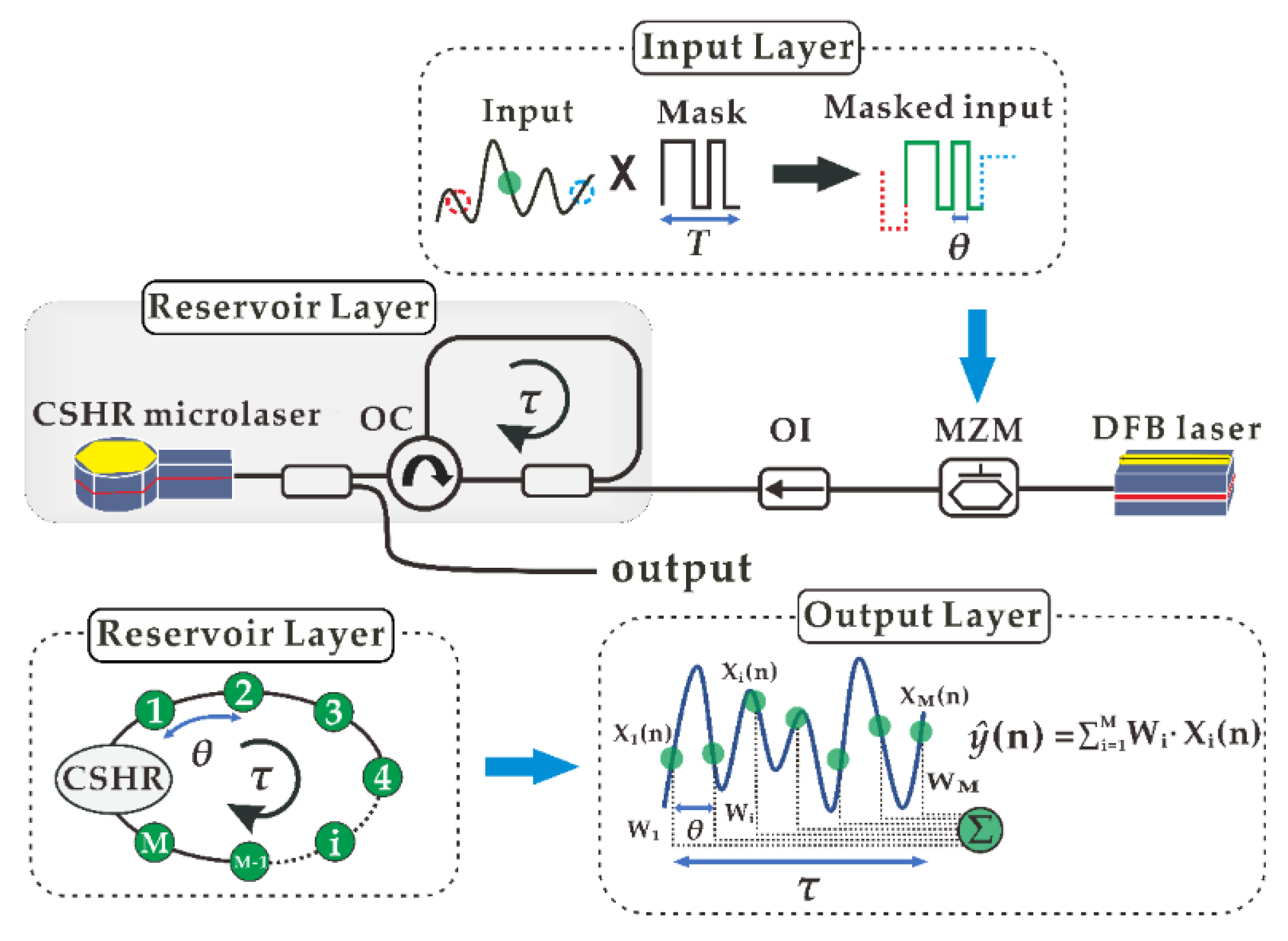
2.2. Model
2.3. Nonlinear Node Characteristics
2.3.1. Modulation Response
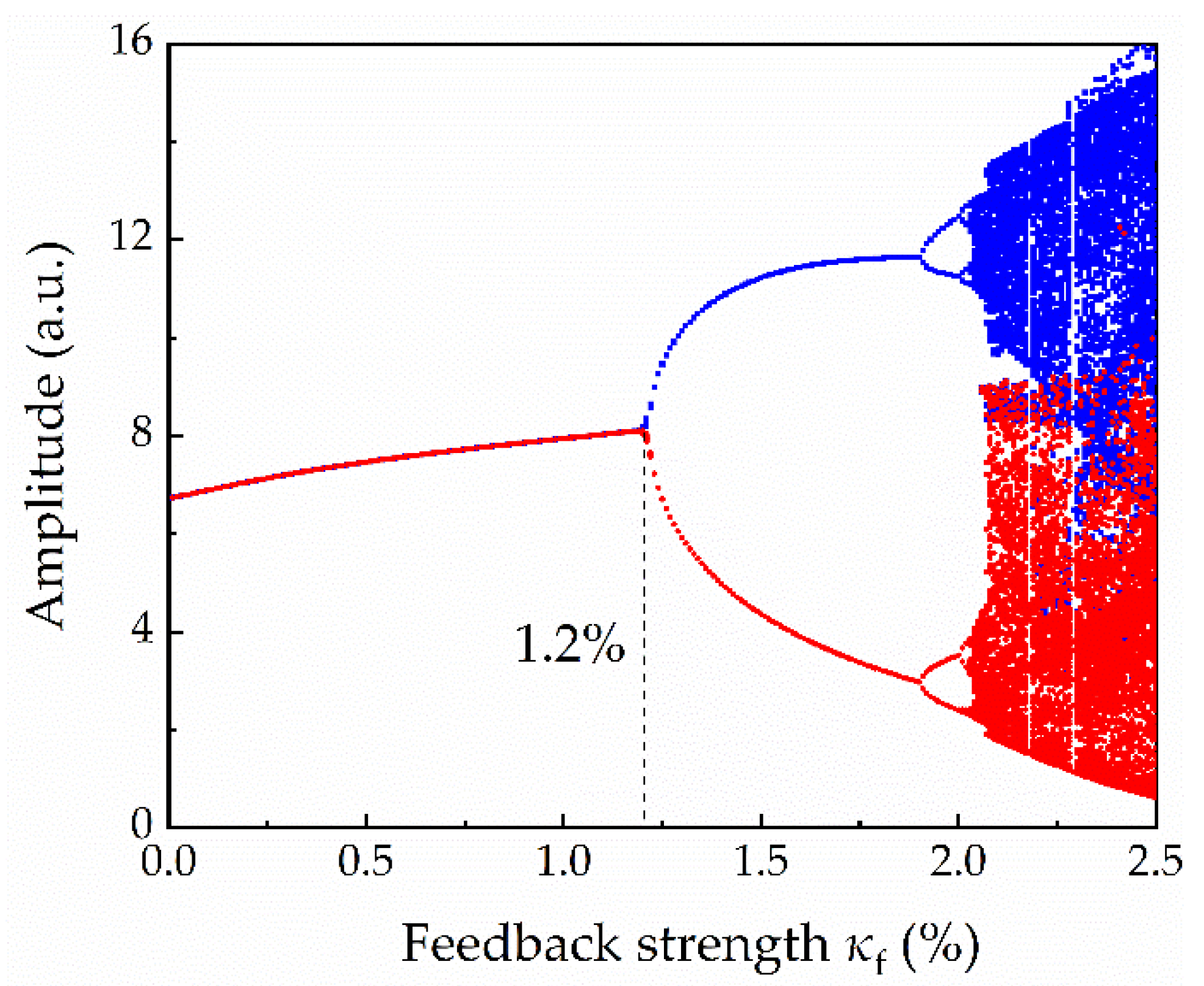
2.3.2. Dynamics
3. Task Test Results and Discussion
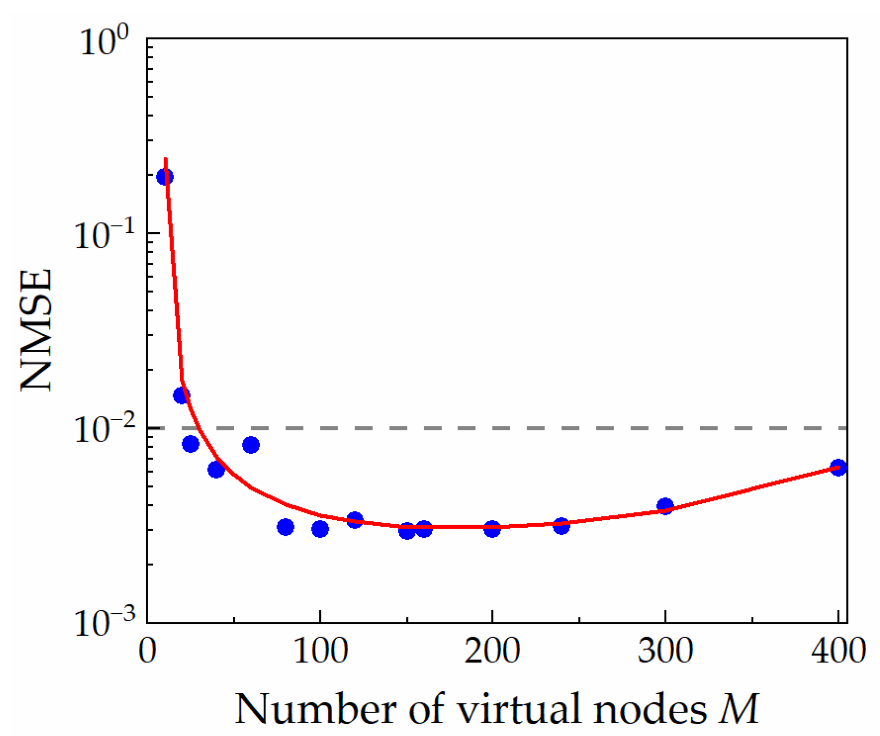
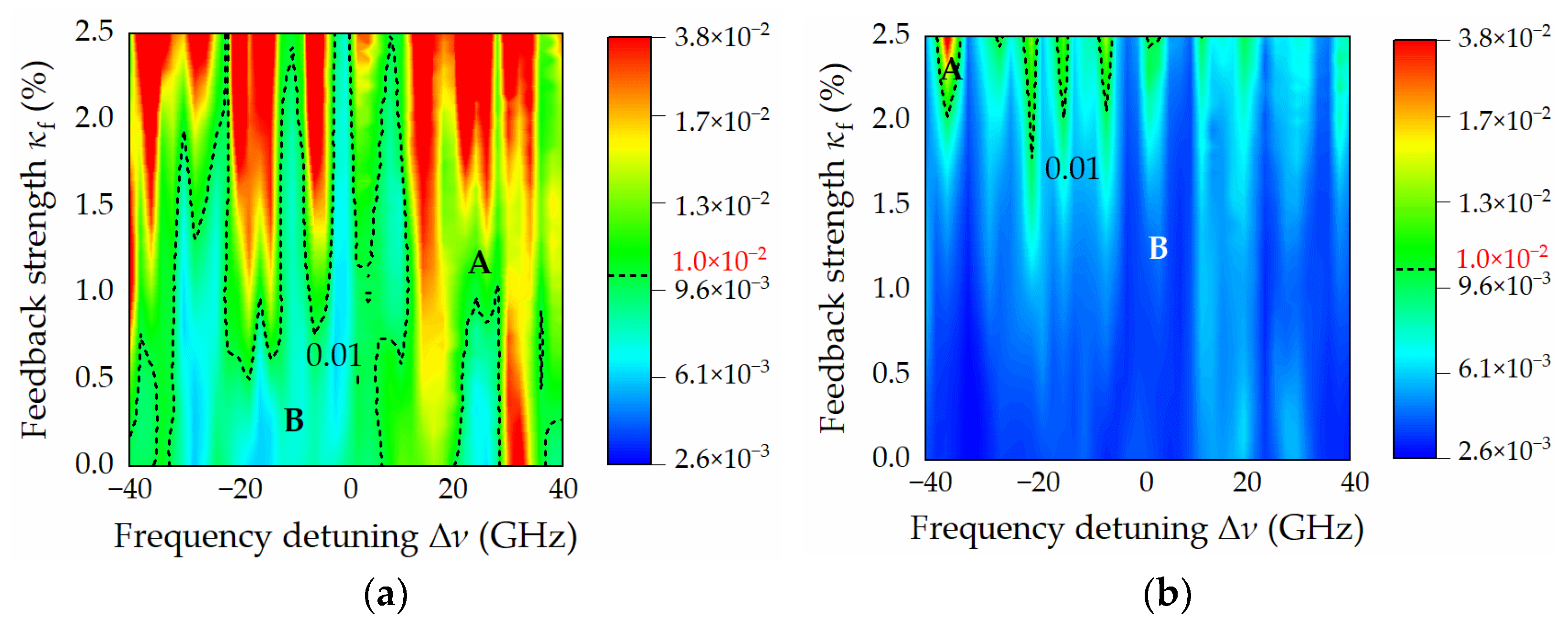
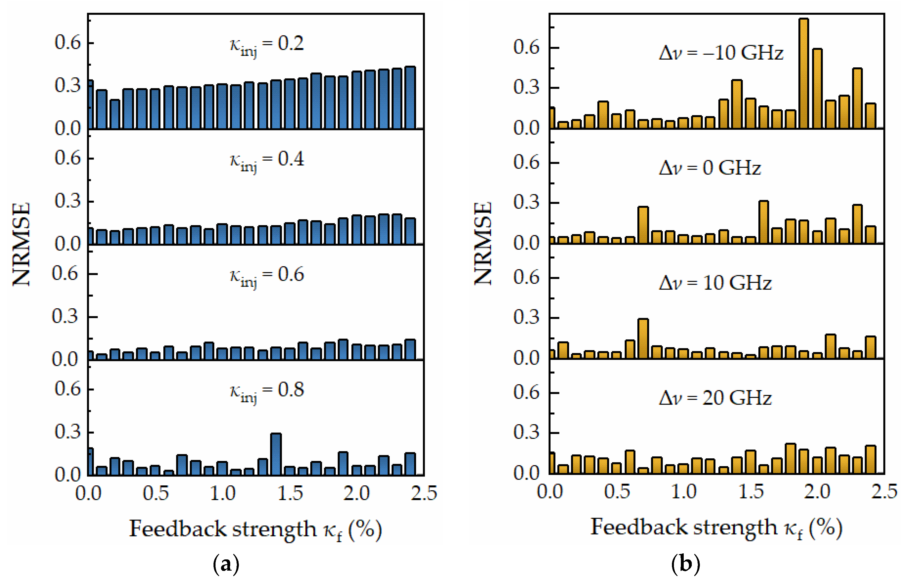
3.1. Santa-Fe Chaotic Time Series Prediction Task
3.2. NARMA-10 Task
3.3. NCE Task
4. Conclusions
Author Contributions
Funding
Data Availability Statement
Acknowledgments
Conflicts of Interest
References
- Lukosevicius, M.; Jaeger, H. Reservoir computing approaches to recurrent neural network training. Comput. Sci. Rev. 2009, 3, 127–149. [Google Scholar] [CrossRef]
- Maass, W.; Natschläger, T.; Markram, H. Real-time computing without stable states: A new framework for neural computation based on perturbations. Neural Comput. 2002, 14, 2531–2560. [Google Scholar] [CrossRef] [PubMed]
- Jaeger, H.; Haas, H. Harnessing nonlinearity: Predicting chaotic systems and saving energy in wireless communication. Science 2004, 304, 78–80. [Google Scholar] [CrossRef] [PubMed] [Green Version]
- Appeltan, M.C.; Soriano, M.C.; van der Sande, G.; Danckaert, J.; Massar, S.; Dambre, J.; Schrauwen, B.; Mirasso, C.R.; Fischer, I. Information processing using a single dynamical node as complex system. Nat. Commun. 2011, 2, 468. [Google Scholar] [CrossRef] [Green Version]
- Haynes, N.; Soriano, M.C.; Fischer, I.; Gauthier, D. Reservoir computing with a single time-delay autonomous Boolean node. Phys. Rev. E 2015, 91, 020801. [Google Scholar] [CrossRef] [Green Version]
- Paquot, Y.; Duport, F.; Smerieri, A.; Dambre, J.; Schrauwen, B.; Haelterman, M.; Massar, S. Optoelectronic reservoir computing. Sci. Rep. 2012, 2, 287. [Google Scholar] [CrossRef]
- Du, W.; Li, C.H.; Huang, Y.X.; Zhou, J.H.; Luo, L.Z.; Teng, C.H.; Kuo, H.C.; Wu, J.; Wang, Z.M. An optoelectronic reservoir computing for temporal information processing. IEEE Electron. Device Lett. 2022, 43, 406–409. [Google Scholar] [CrossRef]
- Kanno, K.; Uchida, A. Photonic reinforcement learning based on optoelectronic reservoir computing. Sci. Rep. 2022, 12, 3720. [Google Scholar] [CrossRef]
- Duport, F.; Schneider, B.; Smerieri, A.; Haelterman, M.; Massar, S. All-optical reservoir computing. Opt. Express. 2012, 20, 22783–22795. [Google Scholar] [CrossRef]
- Estébanez, I.; Li, S.; Schwind, J.; Fischer, I.; Pachnicke, S.; Argyris, A. 56 GBaud PAM-4 100 km transmission system with photonic processing schemes. J. Lightwave Technol. 2022, 40, 55–62. [Google Scholar] [CrossRef]
- Vinckier, Q.; Duport, F.; Smerieri, A.; Vandoorne, K.; Bienstman, P.; Haelterman, M.; Massar, S. High-performance photonic reservoir computer based on a coherently driven passive cavity. Optica 2015, 2, 438–446. [Google Scholar] [CrossRef]
- Brunner, D.; Soriano, M.C.; Mirasso, C.R.; Fischer, I. Parallel photonic information processing at gigabyte per second data rates using transient states. Nat. Commun. 2013, 4, 1364. [Google Scholar] [CrossRef] [PubMed] [Green Version]
- Nguimdo, R.M.; Lacot, E.; Jacquin, O.; Hugon, O.; Van, D.S.G.; Guillet de Chatellus, H. Prediction performance of reservoir computing systems based on a diode-pumped erbium-doped microchip laser subject to optical feedback. Opt. Lett. 2017, 42, 375–378. [Google Scholar] [CrossRef] [PubMed] [Green Version]
- Tanaka, G.; Yamane, T.; Heroux, J.B.; Nakane, R.; Kanazawa, N.; Takeda, S.; Numata, H.; Nakano, D.; Hirose, A. Recent advances in physical reservoir computing: A review. Neural Netw. 2019, 115, 100–123. [Google Scholar] [CrossRef]
- Lugnan, A.; Katumba, A.; Laporte, F.; Freiberger, M.; Sackesyn, S.; Ma, C.; Gooskens, E.; Dambre, J.; Bienstman, P. Photonic neuromorphic information processing and reservoir computing. APL Photonics 2020, 5, 020901. [Google Scholar] [CrossRef]
- Harkhoe, K.; Sande, G.V.D. Task-independent computational abilities of semiconductor lasers with delayed optical feedback for reservoir computing. Photonics 2019, 6, 124. [Google Scholar] [CrossRef] [Green Version]
- Guo, X.X.; Xiang, S.Y.; Zhang, Y.H.; Lin, L.; Wen, A.; Hao, Y. High-speed neuromorphic reservoir computing based on a semiconductor nanolaser with optical feedback under electrical modulation. IEEE J. Sel. Top. Quantum Electron. 2020, 26, 1–7. [Google Scholar] [CrossRef]
- Huang, Y.; Zhou, P.; Yang, Y.; Li, N.Q. High-speed photonic reservoir computer based on a delayed Fano laser under electrical modulation. Opt. Lett. 2021, 46, 6035–6038. [Google Scholar] [CrossRef]
- Estébanez, I.; Schwind, J.; Fischer, I.; Argyris, A. Accelerating photonic computing by bandwidth enhancement of a time-delay reservoir. Nanophotonics 2020, 9, 4163–4171. [Google Scholar] [CrossRef]
- Wang, Y.X.; Jia, Z.W.; Gao, Z.S.; Xiao, J.L.; Wang, L.S.; Wang, Y.C.; Huang, Y.Z.; Wang, A.B. Generation of laser chaos with wide-band flat power spectrum in a circular-side hexagonal resonator microlaser with optical feedback. Opt. Express 2020, 28, 18507–18515. [Google Scholar] [CrossRef]
- Kuriki, Y.; Nakayama, J.; Takano, K.; Uchida, A. Impact of input mask signals on delay-based photonic reservoir computing with semiconductor lasers. Opt. Express 2018, 26, 5777–5788. [Google Scholar] [CrossRef] [PubMed]
- Nakayama, J.; Kanno, K.; Uchida, A. Laser dynamical reservoir computing with consistency: An approach of a chaos mask signal. Opt. Express 2016, 24, 8679–8692. [Google Scholar] [CrossRef] [PubMed]
- Lv, X.M.; Zou, L.X.; Huang, Y.Z.; Yang, Y.D.; Xiao, J.L.; Yao, Q.F.; Lin, J.D. Influence of mode Q factor and absorption loss on dynamical characteristics for semiconductor microcavity lasers by rate equation analysis. IEEE J. Quantum Electron. 2011, 47, 1519–1525. [Google Scholar]
- Ma, X.W.; Huang, Y.Z.; Long, H.; Yang, Y.D.; Wang, F.L.; Xiao, J.L.; Du, Y. Experimental and theoretical analysis of dynamical regimes for optically injected microdisk lasers. J. Lightwave Technol. 2016, 34, 5263–5269. [Google Scholar] [CrossRef] [Green Version]
- Xiao, Z.X.; Huang, Y.Z.; Yang, Y.D.; Xiao, J.L.; Ma, X.W. Single-mode unidirectional-emission circular-side hexagonal resonator microlasers. Opt. Lett. 2017, 42, 1309–1312. [Google Scholar] [CrossRef]
- Uchida, A. Optical Communication with Chaotic Laser; Wiley-VCH Verlag GmbH & Co. KGaA: Weinheim, Germany, 2012; p. 157. [Google Scholar]
- Berre, M.L.; Ressayre, E.; Talleta, A.; Gibbs, H.M.; Kaplan, D.L.; Rose, M.H. Conjecture on the dimensions of chaotic attractors of delayed-feedback dynamical systems. Phys. Rev. A 1987, 35, 4020–4022. [Google Scholar] [CrossRef]
- Yue, D.Z.; Wu, Z.M.; Hou, Y.S.; Hu, C.X.; Jiang, Z.F.; Xia, G.Q. Reservoir computing based on two parallel reservoirs under identical electrical message injection. IEEE Photon. J. 2021, 13, 1–11. [Google Scholar] [CrossRef]
- Jaeger, H. Adaptive nonlinear system identification with echo state networks. In Proceedings of the Conference and Workshop on Neural Information Processing Systems, Vancouver, BC, Canada, 9–14 December 2002. [Google Scholar]
- Rodan, A.; Tion, P. Minimum complexity echo state network. IEEE Trans. Neural Netw. 2010, 22, 131–144. [Google Scholar] [CrossRef]
- Feng, X.X.; Zhang, L.; Pang, X.D.; Gu, X.Z.; Yu, X.B. Numerical study of parallel optoelectronic reservoir computing to enhance nonlinear channel equalization. Photonics 2021, 8, 406. [Google Scholar] [CrossRef]
- Hou, Y.S.; Xia, G.Q.; Jayaprasath, E.; Yue, D.Z.; Wu, Z.M. Parallel information processing using a reservoir computing system based on mutually coupled semiconductor lasers. Appl. Phys. B 2020, 126, 40. [Google Scholar] [CrossRef]


| Symbol | Description | Value |
|---|---|---|
| α | Linewidth enhancement factor | 4 |
| Γ | Confinement factor | 0.25 |
| αi | Internal loss factor | 6 cm−1 |
| c | Velocity of light in vacuum | 3 × 10⁸ m/s |
| ng | Mode group refractive index | 3.5 |
| τpc | Photon lifetime | 8.9 × 10⁻¹² s |
| λ0 | Wavelength | 1550 nm |
| τL | Internal cavity round-trip time | 7.5 × 10⁻¹³ s |
| η | Current injection efficiency | 0.8 |
| Va | Volume of the active region | 30 µm3 |
| A | Defect recombination coefficient | 1 × 10⁸ s−1 |
| B | Radiation recombination coefficient | 1 × 10⁻¹⁰ cm3/s |
| C | Auger recombination coefficient | 1 × 10⁻²⁸ cm6/s |
| Ith | Threshold current | 3.6 mA |
| g0 | Material gain parameter | 1500 cm−1 |
| ε | Gain suppression factor | 18/Ntr |
| Ntr | Transparency density | 1.2 × 1018 cm−3 |
| Ns | Logarithmic gain parameter | 0.92 Ntr |
| Einj,0 | Average amplitude of injected electrical field | 4 × 10¹⁰ |
| bbias | Bias term | 0.5 |
Publisher’s Note: MDPI stays neutral with regard to jurisdictional claims in published maps and institutional affiliations. |
© 2022 by the authors. Licensee MDPI, Basel, Switzerland. This article is an open access article distributed under the terms and conditions of the Creative Commons Attribution (CC BY) license (https://creativecommons.org/licenses/by/4.0/).
Share and Cite
Zhao, T.; Xie, W.; Guo, Y.; Xu, J.; Guo, Y.; Wang, L. High-Speed Reservoir Computing Based on Circular-Side Hexagonal Resonator Microlaser with Optical Feedback. Electronics 2022, 11, 1578. https://doi.org/10.3390/electronics11101578
Zhao T, Xie W, Guo Y, Xu J, Guo Y, Wang L. High-Speed Reservoir Computing Based on Circular-Side Hexagonal Resonator Microlaser with Optical Feedback. Electronics. 2022; 11(10):1578. https://doi.org/10.3390/electronics11101578
Chicago/Turabian StyleZhao, Tong, Wenli Xie, Yanqiang Guo, Junwei Xu, Yuanyuan Guo, and Longsheng Wang. 2022. "High-Speed Reservoir Computing Based on Circular-Side Hexagonal Resonator Microlaser with Optical Feedback" Electronics 11, no. 10: 1578. https://doi.org/10.3390/electronics11101578
APA StyleZhao, T., Xie, W., Guo, Y., Xu, J., Guo, Y., & Wang, L. (2022). High-Speed Reservoir Computing Based on Circular-Side Hexagonal Resonator Microlaser with Optical Feedback. Electronics, 11(10), 1578. https://doi.org/10.3390/electronics11101578