Sensor-System-Based Network with Low-Power Communication Using Multi-Hop Routing Protocol Integrated with a Data Transmission Model

Abstract

Wireless sensor networks (WSNs) comprise several cooperating sensor nodes capable of sensing, computing, and transmitting sensed signals to a central server. This research proposes a sensor system-based network with low power communication using swarm intelligence integrated with multi-hop communication (SIMHC). This routing protocol selects the optimal route based on link distance, transmission power, and residual energy to optimize the network lifetime and node energy efficiency. Moreover, adaptive clustering-based locative data transmission (ACLDT) is applied for optimizing data transmission. The proposed approach combines clustering with data transfer via location-based routing and low-power communication in two phases to calculate the ideal cluster heads (CHs). First, a CH seeks the next hop from the nearest CH. Then, a path to the base station is formed by developing CH chains. The results reveal that the proposed sensor system based on data transmission and low-power consumption achieved a network lifetime of 96%, an average delay of 53 ms, a coverage rate (CR) of 83%, a throughput of 97%, and energy efficiency of 95%.

1. Introduction

A wireless sensor network (WSN) comprises densely spaced and connected by self-organized wireless communication networks. Sensing, embedded computing, signal processing, and wireless networking components are all included in sensor node topologies. Every node is provided with several application-certain sensors and on-node signal processing methods [1]. For example, environmental event detection could benefit from cooperative signal processing among surrounding nodes, increasing detection sensitivity and specificity. Users can receive locally processed information via energy significant wireless transmission. Low power consumption is critical for a WSN to have a long operating lifetime. Multi-hop networking among SN is presented to lower the communication connection range for every node in SN [2], which is aided by low duty cycle process and local signal processing. Because communication channel loss scales as a power law with the link range, reducing the link range results in enormous savings. Initially, WSNs were utilized for military purposes, such as battlefield monitoring, but are now employed for various applications. Depending on the application, the WSN might have hundreds to thousands of nodes, all of which may be connected in a network. Each node comprises a radio transceiver with an internal or external antenna, microprocessor, electronic circuit for sensor interface, and power source, such as batteries [3]. The nodes utilized in a WSN are typically small and powered by batteries or solar panels [4]. There are network lifetime extensions and energy-efficient data transmission. In most applications, batteries are powered by batteries, which utilize little energy due to their limited energy supply [5].

The aims of this work are described as follows:

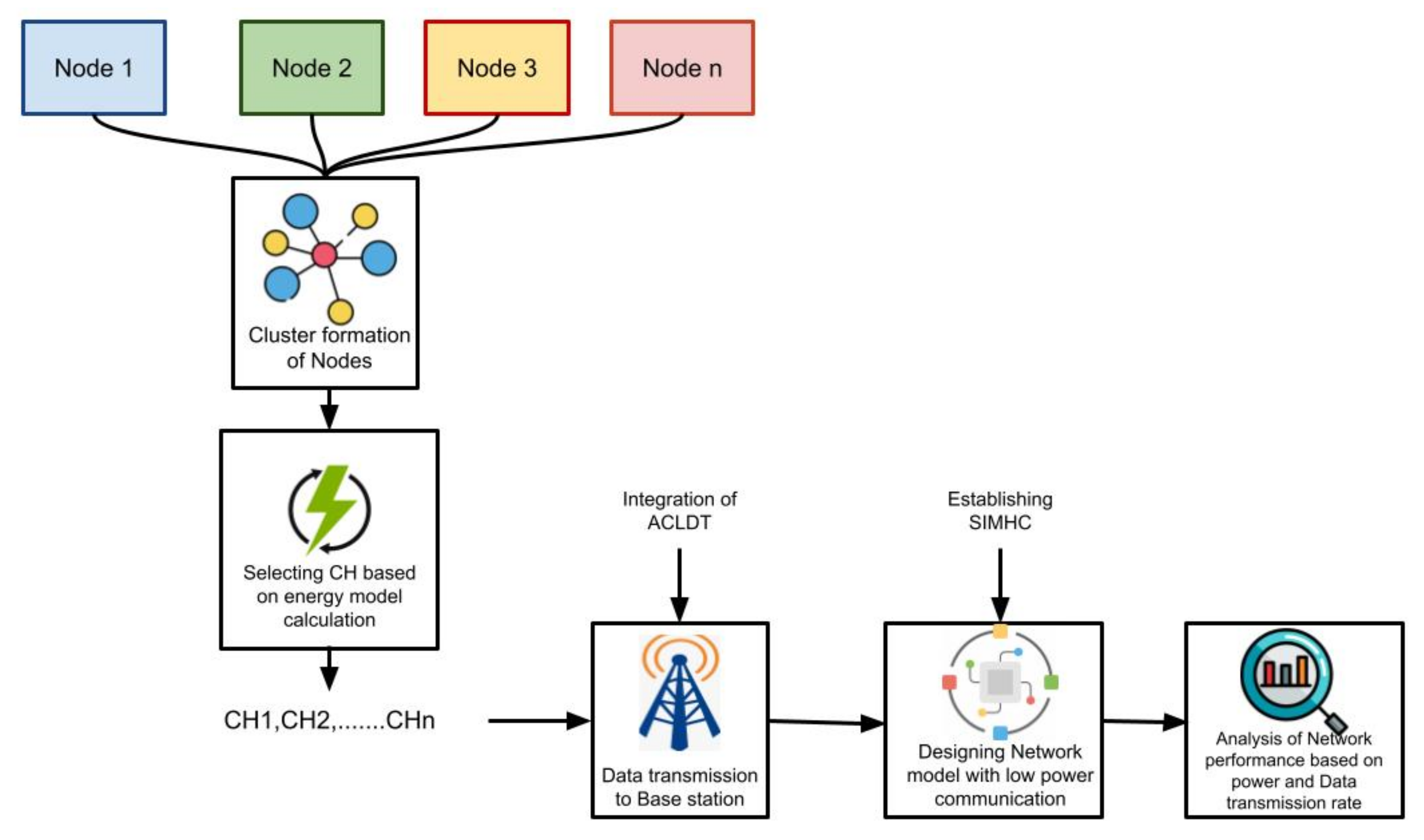
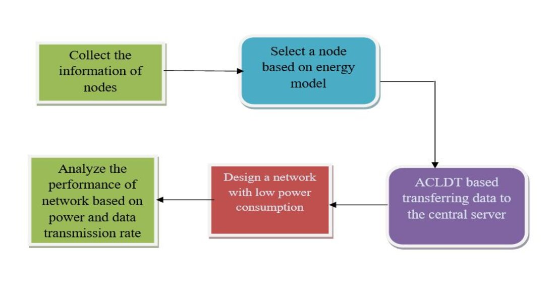
• Design a sensor system and network based on low power communication with data transmission.
• Integrate multi-hop communication with swarm intelligence to achieve low-power communication.
• Cluster the nodes and calculate optimal cluster heads with data transmission.
• Apply the adaptive clustering-based locative data transmission algorithm for data transmission, where the exact locations of the sink node and base station are known.

The rest of this research is organized as follows. Section 2 discusses existing WSN techniques based on a sensor system with a network model. Section 3 explains the proposed system method, including the energy model, clustering and cluster head selection evaluation, data transmission model, and low power transmission model. Section 4 presents the experimental results based on parametric data transmission analysis and low power consumption evaluation. Finally, Section 5 concludes the research and describes the direction of future work.

2. Related Works

Many routing protocols, such as hierarchical, flat and location types, are designed to fit WSN features, in which energy is a critical problem. Other available routing protocols include data-centric routing protocols, such as SPIN and directed diffusion, and those for low-power and lossy networks. Signal strengths anticipate the distance between nodes, so the nodes are aware of their locations [6]. Geographical and energy-aware routing (GEAR) [7] is a technique for routing packets to a destination region that incorporates energy-aware neighbor selection. Cluster-based routing was created with scalability and communication in mind, and the formation of clusters as well as selection of CHs can extend a network’s lifespan [8]. Because the energy capacity is limited [9], conserving energy is significant in determining the sensor network’s lifespan. Many strategies for extending the life of a network have been presented, such as the LEACH [10] technique, in which SNs send data to a CH rather than to the base station (BS) directly. The LEACH approach has been modified numerous times and has become a core method among hierarchical routing systems. For instance, the LEACH protocol, a variation of the LEACH technique that incorporates location and residual energy characteristics, was created to address the issue of load balancing with low degrees [11]. The TL-LEACH protocol is another method for resolving the distance problem between CHs and BSs [12]. The LEACH methodology is also used for CH data gathering and fusion, although one CH uses another CH closer to BS. The power-efficient gathering in sensor information system (PEGASIS) [13] is another protocol in which nodes only communicate with their nearest neighbors. To ensure all nodes have the BS, sensing node systems use a greedy algorithm to establish transmission chains. V-LEACH [14], a highly energy-efficient variation of LEACH, is another option. In the CH selection step, the distributed EEUC method [15] considers node energy usage and distance between source and sink nodes to equalize the network’s energy consumption by marking all nodes. The CUCA algorithm [16] selects the cluster head, considering the distance factor, network coverage, and node residual energy. CH in the ERA method [17] creates multi-path data transmission based on residual energy; however, inducing the energy hole to appear prematurely is trivial. Regiment Al [18] suggested a distributed fuzzy logic method based on energy perception as well as CR with non-uniform cluster heads. Yet, the non-uniformity of CHs cannot match the network’s reduced energy consumption and maximum CR standards. Subsequently, a distributed multi-layer DFCR clustering technique [19] with improved big data transmission performance was suggested in 2018. The DFCR algorithm considers the nodes’ degree, residual energy, distance, centrality, and other characteristics before constructing a multi-objective optimization method to address the uneven energy consumption of nodes. The target tracking issue over a filtering network with dynamic cluster and data fusion is the subject of this research [20]. The clustering technique has been further enhanced for specific real applications over the last two years and has obtained good results [21,22].

3. System Model

This section discusses the designed sensor system and network based on low-power communication with data transmission. Here, the proposed model is classified into two modules. The first module includes node clustering and selection of the cluster with data transmission by adaptive clustering-based locative data transmission (ACLDT). The second module involves low-power communication using swarm intelligence integrated with multi-hop communication (SIMHC). The proposed model is represented in Figure 1.

3.1. Energy Model

The following equation is used to calculate the transmitting, receiving and aggregating data of energy consumption:

$$E_{tr}\left(l\right)=\left\{\begin{array}{ll}{E}_{\mathrm{elec} }+l·{\epsilon }_{fs}·d^2\hfill & d\le d_0,\hfill \\ E_{\mathrm{elec} }+l·{\epsilon }_{mp}·d^4\hfill & d>d_0,\hfill \end{array}\right.E_{rx}\left(l\right)=l{E}_{\mathrm{elec} }.$$

(1)

$$E_{ag}\left(l\right)=l{E}_{da}$$

where d is the distance from the source node to Sink; $d_0=\sqrt{\frac{{\epsilon }_{fs}}{{\epsilon }_{mp}}}; E_{tx}\left(l\right), E_{rx}\left(l\right), E_{ag}\left(l\right)$ for aggregating 1 bit of data; E_da reflects the energy use; ${\epsilon }_{fs}$ and ${\epsilon }_{mp}$ represent the signal amplifier power magnifications in free-space and multi-channel attenuation models, respectively; and $\mathrm{Emelec}$ denotes the energy usage of a wireless transceiver circuit in transmitting and receiving data. If d ≤ d₀, the network’s communication model is a free-space method; otherwise, it is a multi-channel attenuation method modeled by Equation (2):

$$\begin{array}{l}{\sum }_{i=1}^N{E}_i={\sum }_{i=1}^K\left[E_m\right({\sum }_{j=1}^{K+1}{I}_{ij}-{\sum }_{j=1}^K{I}_{ji})+{\sum }_{j=1}^{K+1}{E}_{ij}+{\sum }_{j=1}^K{E}_m{I}_{j_i}]\\ \hspace{1em}\hspace{1em}\hspace{1em}\hspace{1em}\hspace{1em}\hspace{1em}\hspace{1em}=E_{sm}{\sum }_{i=1}^K{I}_{iK+1}+{\sum }_{i=1}^K{\sum }_{j=1}^{K+1}{E}_{ij}+E_n{\sum }_{i=1}^K{\sum }_{j=1}^K{I}_{ij}\\ \hspace{1em}\hspace{1em}\hspace{1em}\hspace{1em}\hspace{1em}\hspace{1em}\hspace{1em}={\sum }_{i=1}^K\left(E_{sm}{I}_{iK+1}+E_{iK+1}\right)\\ \hspace{1em}\hspace{1em}\hspace{1em}\hspace{1em}\hspace{1em}\hspace{1em}\hspace{1em}+{\sum }_{i=1}^K{\sum }_{j=1}^K\left(E_{rc}{I}_{ij}+E_{ij}\right)m{\displaystyle \sum _{i=1}^K}\left(E_{\mathrm{sm}}{I}_{iK+1}+E_{iK+1}\right)\\ \hspace{1em}\hspace{1em}\hspace{1em}\hspace{1em}\hspace{1em}\hspace{1em}\hspace{1em}+{\displaystyle \sum _{i=1}^K}{\displaystyle \sum _{j=1}^K}\left(E_n{I}_{ij}+E_{ij}\right)\end{array}$$

(2)

such that,

$${\displaystyle \sum }_{j=1}^{K+1}{I}_{ij}-{\displaystyle \sum }_{j=1}^K{I}_{ji}\ge 0$$

for $i=1:K$ and from Equation (3)

$${\displaystyle \sum }_{j=1}^{K+1}{I}_{lj}-{\displaystyle \sum }_{j=1}^K{I}_{jj}\le M{\displaystyle \sum }_{j=1}^K{I}_{jK+1}$$

(3)

for $i=1:K$, Equation (4) is

$${\displaystyle \sum }_{j=1}^K{I}_{jK+1}\ge I_{\min }$$

(4)

which becomes Equation (5)

$$I_{ij}\le \log \left(1+\frac{E_{ij}{d}_{ij}^{-2}}{\zeta }\right)$$

(5)

for $i=1:K,j=1:K+1$, which is rewritten as Equation (6):

$$I_{ij}\ge 0;E_{ij}\ge 0$$

(6)

for $i=1:K,j=1:K+1$.

Equations (5) and (6) are used to compute the maximum energy bounds ranging from ESP ¼ 1 Joule to ESP ¼ 15 Joules and fewer data bounds ranging from Imin ¼ 0 to Imin ¼ 170 bits, respectively. The network is randomly distributed with 100 nodes with Erc ¼ 500 μJ, Esm ¼ 1 mJ, and M ¼ 20 bits based on the relationship between Equations (5) and (6). The problem with the minimum data bound in Equation (6) is that it converges faster than the issue with high energy bound in Equation (5).

3.2. Clustering and Selection of Cluster Heads

First, we determine the expected distances between CHs and SINK using an integral, then the expected distances between CHs and nodes inside its cluster. Then, the entire predicted energy consumption value is calculated to obtain the ideal number of cluster heads. The node density denotes the tightness of the relationships between the activity nodes and displays the difference between a complete graph and a distribution graph. In the following method, we choose the best CHs by considering node energy consumption, degrees, and distances, as shown in Algorithm 1. Assume that the network contains k clusters and N nodes. Under the free-space model, network’s energy consumption is given by Equation (7):

$$E_{CH}=\left(\left|\frac{N}{k}\right|-1\right)·l·E_{\mathrm{lec} }+\frac{N}{k}·l·E_{\mathrm{da} }+l·E_{\mathrm{lec} }+l·{\epsilon }_{fs}·DCH-Sin$$

(7)

where $d_{CH-Sink}^2$ is the estimated distance between CH and Sink, $\left|\frac{N}{k}\right|;\left(\left|\frac{N}{k}\right|-1\right)$ is the average number of nodes in each cluster, and $E_{\mathrm{lec} }$ denotes the amount of energy used by CH to receive $\left(\left|\frac{N}{k}\right|-1\right)$ bits of data. The energy usage for CH to transmit l bit of data is represented as $l·E_{\mathrm{lec} }+l·{\epsilon }_{fs}{d}_{CH-Sink}^2$. In a free-space model, the best CH location is (x, y), while the Sink’s coordinate is (x, y) (a, b). As a result, the following equation is the expected squared distance between the CH and Sink:

$$\begin{gathered} E\left[d_{CH-Sink}^2\right]=\iint \left({(a-x)}^2+{(b-y)}^2\right)d_{CH}\left(x,y\right)\mathrm{d}x\mathrm{d}y \\ =\iint \frac{{(a-x)}^2+{(b-y)}^2}{S}\mathrm{d}x\mathrm{d}y \end{gathered}$$

(8)

The $\left(x,y\right)$ is the distance between source node and CH, and S is the square area of the node distribution. Consider that each cluster contains l bit of data to be conveyed. Then, Equation (9) is used to determine the energy usage of one cluster in one round:

$$E_{CH-members}=l·E_{elec}+l·{\epsilon }_{fs}{}_{DCH-members}^2$$

(9)

Within a cluster, the expected squared distance from CH to the source node is given by Equation (10):

$$E\left[d_{CH-members}^2\right]=\iint \left(x^2+y^2\right)d\left(x,y\right)\mathrm{d}x\mathrm{d}y=\frac{L^2}{2\pi k}$$

(10)

To begin, determine whether node vi is a cluster head by calculating the following:

$$C{H}_{\mathrm{Candidate}-\mathrm{i} }=\alpha ·\left(\frac{E_{\mathrm{Remain}-\mathrm{i} }}{E_{\mathrm{Initial} }}\right)+\beta ·\left(\frac{Deg \max }{De{g}_i}\right)+\gamma ·\left(\frac{Di{s}_{i-Sink}}{Di{s}_{\max }-Sink}\right)$$

(11)

where α, β, and γ are parameters that satisfy 0 < α, β, γ < 1, α + β + γ = 1;$E_{\mathrm{Remain}-\mathrm{i} }$ represents the remaining energy of node vi; $\mathrm{initial}$ is the initial energy of all nodes; $De{g}_i$ is the degree of node vi; Deg max denotes the maximum degree of all nodes; $Di{s}_{i-Sink}$ refers to the distance between node vi and Sink; and $Di{s}_{\max }-Sink$ is the greatest distance between the source node and Sink. Candidate set $C{H}_{\mathrm{Candidate}-\mathrm{i} }$ is created by sorting the candidate values from high to low using the aforementioned algorithm. When the network’s minimal CR is equal to or greater than 90%, the best CH is chosen from the candidate sets.

Algorithm 1: Clustering and CH Selection

Need:

N denotes number of alive nodes

V(I, j), I, j = 1, 2…..N

S(a,b)

Neighbor vi{}

r denotes node transmission range

Confirm:

List CH{i\i = 1,…,Not-CH

1.  State List CH {} = NULL

2.  Evaluate candidate value of node vi as a CH

3.  For I = 1 to N do

4.  N = +1

5.  If n is not equal to Not-CH, then

6.  For j = i + 1 to N, do

7.  If CR < 90%, then

8.  Choose next node vj

9.  End if

10.   End for

3.3. Adaptive Clustering-Based Locative Data Transmission (ACLDT)

To characterize data evolution in ACLDT, the data transmission method trusts on building an initial identical predictive method at theCH and SN. It is worth mentioning that each CH or BS should perform ACLDT for each node to which it is connected. The query made by a user is analyzed and replied to, using the created predictive methods at the CH connecting with SN, which satisfies the quality based on a given boundary. Furthermore, a direct connection between SN and CH is required to update models at CH if the method is not accurate enough. The actual sensor values must be received in this situation, and the prediction model must be updated at both the CH and SN. It is pertinent to mention that an identical scenario is used to communicate between the CH and BS. When using a power line connection, all nodes are energy balanced. Each node can consider the overall energy optimization when choosing a data transmission channel, as shown in Algorithm 2. The data from a node that is further away from the BS are present in numerous hops to the BS. A node that is d meters away from BS emits 1 bit of data, which is routed through n hops to the base station, where $E_{\mathrm{bit}}\left(d, n\right)$ is the entire amount of energy used in this process, as shown in Equation (12):

$$E_{\mathrm{bit}}\left(d,n\right)=n\times E_T+\left(n-1\right)\times \left(E_{\mathrm{R}}+E_{\mathrm{DA}}\right)=\left\{\begin{array}{c}n\times \left(E_{\mathrm{elec}}+{\epsilon }_{\mathrm{fs}}\times {\left(\frac{d}{n}\right)}^2\right)+\\ \left(n-1\right)\times \left(E_{\mathrm{elec}}+E_{\mathrm{da}}\right),\frac{d}{n}<d_0\\ n\times \left(E_{\mathrm{elec}}+{\epsilon }_{\mathrm{amp}}\times {\left(\frac{d}{n}\right)}^4\right)+\\ \left(n-1\right)\times \left(E_{\mathrm{elec}}+E_{\mathrm{da}}\right),\frac{d}{n}\ge d_0\end{array}\right.$$

(12)

Algorithm 2: ACLDT

Input:

Input sensor readings x

Initialization: start = 1,

While t < T do, $\lambda =0,$ ws, wf, $\alpha$, emax

$\begin{array}{l}{\widehat{y}}_f\leftarrow \frac{1}{w_f}{\displaystyle \sum _{i=t-w_{f+1}}^{t-1}}{x}_e\left(i\right);\\ {\widehat{y}}_s\leftarrow \frac{1}{w_s}{\displaystyle \sum _{i=start}^{t-1}}{x}_e\left(i\right);\\ \widehat{y}\left(t\right)\leftarrow \lambda \left(t\right){\widehat{y}}_f+\left[1-\lambda \left(t\right)\right]{\widehat{y}}_s;\\ e\left(t\right)\leftarrow x_e\left(t\right)-\widehat{y}\left(t\right);\\ w\leftarrow {\widehat{y}}_f-{\widehat{y}}_s;\end{array}$

If |e(t)| < emax, for ws consecutive steps and no ACK is neededthen

$\begin{array}{l}{x}_e\left(t\right)=\widehat{y}\left(t\right);\\ \lambda \left(t+1\right)\leftarrow \lambda \left(t\right);\\ else\\ x_e\left(t\right)=x\left(t\right);\\ \lambda \left(t+1\right)\leftarrow \lambda \left(t\right)+\alpha e\left(t\right)w;\\ \mathrm{start} \leftarrow t;\end{array}$

T = t + 1

3.4. Low-Power Communication Using Swarm Intelligence Integrated with Multi-Hop Communication (SIMHC)

In general, the overall power consumption in the WSN is divided into two parts, PPA and Pc, as shown in Equations (13) and (14):

$$P_{\mathrm{PA}}\left(d\right)=\left(1+\alpha \right)P_{\mathrm{out}}\left(d\right)$$

(13)

where α is the drain efficiency.

$$P_{\mathrm{out} }\left(d\right)={\stackrel{\leftharpoonup }{E}}_{\mathrm{b}}{R}_{\mathrm{b}}\frac{{(4\pi )}^2{d}^{\beta }{M}_{\mathrm{l}}{N}_f}{G_{\mathrm{t}}{G}_{\mathrm{r}}{\lambda }^2}$$

(14)

where $R_{\mathrm{b}}$ denotes bit rate;$G_{\mathrm{t}}$ stands for the transmitter antenna gain; and $G_{\mathrm{r}}$ represents the reception antenna gain; d is the transmission distances;$M_{\mathrm{l}}$ indicates the link margin; β is the path-loss exponent; and $N_f$ denotes the power spectral density. Energy per bit for a particular BER, E_b, is evaluated using the following equation:

$$\begin{gathered} {\stackrel{\leftharpoonup }{P}}_{\mathrm{b}}=\frac{4}{b}\left(1-\frac{1}{2^{b/2}}\right)\frac{1}{2^{N_{\mathrm{T}}{N}_{\mathrm{R}}}}{\left(1-\frac{1}{\sqrt{1+2N_{\mathrm{o}}/E_{\mathrm{b}}}}\right)}^{N_{\mathrm{T}}{N}_{\mathrm{R}}} \\ \hspace{1em}\hspace{1em}\hspace{1em}\hspace{1em} \times {\sum }_{k=0}^{N_{\mathrm{T}}{N}_{\mathrm{R}}-1}\frac{1}{2^{\beta }}\left(\begin{array}{c}{N}_{\mathrm{T}}{N}_{\mathrm{R}}-1+\beta \\ \beta \end{array}\right)\times {\left(1+\frac{1}{\sqrt{1+2N_{\mathrm{o}}/E_{\mathrm{b}}}}\right)}^{\beta } \end{gathered}$$

(15)

where P_b stands for the BER, which is the number of SNs; NR denotes number of receiver nodes; and b is size of the constellation, which is calculated using Equation (16).

$$\begin{gathered} P_C=N_{\mathrm{T}}\left(P_{\mathrm{mix} }+P_{\mathrm{DAC}}+P_{\mathrm{filt} }\right)+2P_{\mathrm{synth} } \\ \hspace{1em}\hspace{1em}\hspace{1em}\hspace{1em}\hspace{1em}\hspace{1em}+N_{\mathrm{R}}\left(P_{\mathrm{mix} }+P_{\mathrm{LNA}}+P_{\mathrm{IFA}}+P_{\mathrm{filr} }+P_{\mathrm{ADC}}\right) \end{gathered}$$

(16)

where $P_{\mathrm{DAC}}$ and $P_{\mathrm{ADC}}$ are the power consumed by digital-to-analogue and analogue-to-digital converters, respectively; $P_{\mathrm{filt}}$ and $P_{\mathrm{filr} }$ indicate transmitter and receiver end filters;$P_{\mathrm{mix}}$ refers to the power consumed by the mixer;$P_{\mathrm{synth} }$ is the power consumed by the frequency synthesizer; $P_{\mathrm{LNA}}$ denotes the power consumed by the low noise amplifier; and $P_{\mathrm{IFA}}$ is the power consumed intermediate frequency of SN. Then, the overall energy consumption per bit becomes

$$E_{\mathrm{pb}}=\frac{P_{\mathrm{PA}}+P_{\mathrm{c}}}{R_{\mathrm{b}}}$$

(17)

R_b can be altered by setting $R_{\mathrm{b}}^{\mathrm{eff}}=R_{\mathrm{b}}\frac{\left(F - p{N}_{\mathrm{T}}\right)}{F}$, where $p{N}_T$ training models are inserted in each block. Specifically, TC refers to the fading coherence time, and RS is the symbol rate. For the greatest Doppler shift, $T_{\mathrm{C}}=3/4f_m\sqrt{\pi }$ is coherence time T (FM) = v/λ, where v signifies the velocity. When $p{N}_T$ training symbols are presented in each block, the overall energy usage per bit is as given by Equation (18):

$$E_{\mathrm{pbt}}=\frac{F}{\left(F-p{N}_T\right)}\left[\frac{P_{\mathrm{PA}}+P_{\mathrm{c}}}{R_{\mathrm{b}}}\right]$$

(18)

The letter p denotes the overhead training factor. A 2 × two virtual MIMO link connects all CGs to the next master CG. As a result, the per-bit energy usage is given by Equation (19):

$$E_{\mathrm{pbt}}^{\mathrm{DSC}-\mathrm{MIMO}}\left(d\right)=\frac{F}{\left(F-p{N}_{\mathrm{T}}\right)}\left[{\left.E_{\mathrm{pb}}\left(d\right)\right|}_{N_{\mathrm{T}}=2,N_{\mathrm{R}}=2}\right]R_{X1}$$

(19)

Particles in a swarm-based algorithm update their position about a group’s position and velocity. The i-th particle $P_i$ of n D-dimensional population is represented as

$$P_i=\left[X_{i,1},X_{i,2},X_{i,3}\dots ,X_{i,D}\right]$$

(20)

The position of each particle is assessed by utilizing a fitness function that assesses the quality of the answer it provides in that iteration. For each particle’s velocity and location, the $V_i$ and $X_i$ can be updated by Equation (21):

$$V_{\mathrm{new} ,i}=w\ast V_i+c_1\ast r_1\ast \left({ \mathrm{Xpbest} }_i-X_i\right)+c_2\ast r_2\ast \left(X_{gbest}-X_i\right)$$

(21)

where w stands for the inertia weight; c₁ and c₂ are acceleration factors; and r₁ and r₂ are random values in the range [0, 1].

$$w=w_{\mathrm{initial} }-\frac{ \mathrm{Max}. \mathrm{Iteration} - \mathrm{Current} \mathrm{Iteration} }{ \mathrm{Total} \mathrm{Number} \mathrm{of} \mathrm{Iterations} }$$

(22)

$$\mathrm{New}i,j=X_{\mathrm{old},i}+V_{\mathrm{new},i}$$

To produce the optimal number of CHs, a swarm-based approach is used. The value of the inertia weight is evaluated in the proposed PSO method, utilizing Equation (22), which is a time-varying operation that yields distinct values for every iteration. Furthermore, if an SN is within its communication range, it can be used as a CH. The core knowledge concept is similar to traditional algorithms, such as LEACH. Every node delivers data to the CH at the start of each new iteration. Facts are aggregated, redundant data are deleted, and remaining data are passed onto the next hop, CH or BS, as shown in Algorithm 3.

Reff b and Rb are related by Equations (23) and (24):

$$\begin{gathered} E_{\mathrm{pbt}}=\frac{F}{\left(F-p{N}_{\mathrm{T}}\right)}\left[\frac{P_{\mathrm{PA}}+P_{\mathrm{c}}}{R_{\mathrm{b}}}\right]E_{\mathrm{pbt}}=\frac{3\lambda R_{\mathrm{S}}}{\left(3\lambda R_{\mathrm{S}}-4vp{N}_{\mathrm{T}}\sqrt{\pi }\right)}\left[\frac{P_{\mathrm{PA}}+P_{\mathrm{c}}}{R_{\mathrm{b}}}\right] \\ {R}_{\mathrm{b}}^{\mathrm{eff}}=\frac{F-p{N}_{\mathrm{T}}}{F}{R}_{\mathrm{b}}=\frac{T_{\mathrm{c}}{R}_{\mathrm{s}}-p{N}_{\mathrm{T}}}{T_{\mathrm{c}}{R}_{\mathrm{s}}}=\frac{\frac{3}{4f_m\sqrt{\pi }}{R}_{\mathrm{s}}-p{N}_{\mathrm{T}}}{\frac{3}{4f_m\sqrt{\pi }}{R}_{\mathrm{s}}}{R}_{\mathrm{b}}\frac{3\lambda }{4v\sqrt{\pi }}{R}_{\mathrm{s}}-p{N}_{\mathrm{T}} \end{gathered}$$

(23)

$$\begin{gathered} \mathrm{Velocity} \left(v\right)=\frac{3\lambda }{4v\sqrt{\pi }}{R}_{\mathrm{s}}\mathrm{or} \frac{R_{\mathrm{b}}^{\mathrm{eff}}}{R_{\mathrm{b}}}=1-\frac{p{N}_{\mathrm{b}}}{\frac{3\lambda }{4v\sqrt{\pi }}{R}_{\mathrm{s}}} \\ \frac{3p{N}_{\mathrm{T}}\sqrt{\pi }}{2}\left(1-\frac{R_{\mathrm{b}}^{\mathrm{eff}}}{R_{\mathrm{b}}}\right). \end{gathered}$$

(24)

When $p{N}_{\mathrm{T}}$ training models are introduced in each block, the overall energy usage per bit is given by Equations (25) and (26):

$$E_{\mathrm{pbt}}=\frac{F}{\left(F-p{N}_{\mathrm{T}}\right)}\left[\frac{P_{\mathrm{PA}}+P_{\mathrm{c}}}{R_{\mathrm{b}}}\right]$$

(25)

$$E_{\mathrm{pbt}}=\frac{3\lambda R_{\mathrm{S}}}{\left(3\lambda R_{\mathrm{S}}-4vp{N}_{\mathrm{T}}\sqrt{\pi }\right)}\left[\frac{P_{\mathrm{PA}}+P_{\mathrm{c}}}{R_{\mathrm{b}}}\right]$$

(26)

For a given carrier frequency, block size (F) will remain constant if the velocity is constant. As a result, the value of p at the boundary is determined by F-pNT, and the boundary condition is p F/NT. Because the value of p does not satisfy the boundary condition, the overall energy usage becomes unfavorable.

Algorithm 3: SIMHC

Step 1: initializing the network by putting $n$ node in $p$ zone randomly

Step 2: select a cluster head for each of the zones randomly

while (finish energy of nodes or finish number of rounds)in each of zones

Step 3: compare fitness for all of the nodes

while (find the best fitness)

$\{$ if (fitness (node $\left(i\right))>$ fitness $\left(\mathrm{CH}\right))$

change the $\mathrm{CH}$

}else$\{$ remove nodes inside event radiusadd new nodes and put randomly

}

Step 4: new placement of nodes based on $\mathrm{CH}$

} Step 5: send data from sensor node to $\mathrm{CH}$

Due to the (energy and buffer size of a node) send data based on nearest neighbour node

Step 6: send data from $\mathrm{CH}$ node to sink

1   Set $\mathrm{Set} w,c1,c2$ and $c3$ parameters

2   Initialize particles $P_i,i,j,1\le i\le NP,1\le j\le D=m$

3   Evaluate fitness $\left(P_i\right)$ of every particle and determine the best position of the particle as well as set it to ${\mathrm{pbest} }_i$

4   Evaluate global best position of the particle.

$\mathrm{Gbest} =\left\{{ \mathrm{Pbest} }_{\mathrm{k}}\mid \mathrm{Fitness} \left({ \mathrm{Pbest} }_{\mathrm{k}}\right)=\mathrm{m}\left( \mathrm{Fitness} \left({ \mathrm{Pbest} }_{\mathrm{i}}\mid \right),\mathrm{i},1\le \mathrm{i}\le \mathrm{NP}\right)\right\}$

5   Update velocity and position of $P_i$ and evaluate Fitness $\left(P_i\right)$

6   If Fitness $\left(P_i\right)<$ Fitness $\left.\left(P\right.{ \mathrm{best} }_i\right)$ then $P{ \mathrm{best}}_i=P_i$

7   If Fitness $\left(P_i\right)<$ Fitness (Gbest) then Gbest $=P_i$

8   Repeat steps 3–7 until stopping criteria are not met.

4. Performance Analysis

R2016b MATLAB software was used to mimic the features, settings, and data. The following characteristics were used in this study: Intel Core i7 3.2 GHz processor, 16 GB RAM and Windows 10. MATLAB software provides various mathematical advantages over other applications, including the ability to share source codes across users, and thus was chosen to simulate the proposed method—the simulation parameters are represented in

Table 1. Simulation parameters.

Parameter	Value
Field size	100 × 100 m2
Number of sensor nodes	100
Energy of sensor nodes	80% have 2J; 20% have 5J
Base Station location	(0,0)
Number of clusters	9
Size of message	4000 bits

.

Table 2. Comparative analysis of proposed sensor system and network based on low-power communication and existing techniques.

Parameters	LEACH	PEGASIS	SIMHC_ACLDT
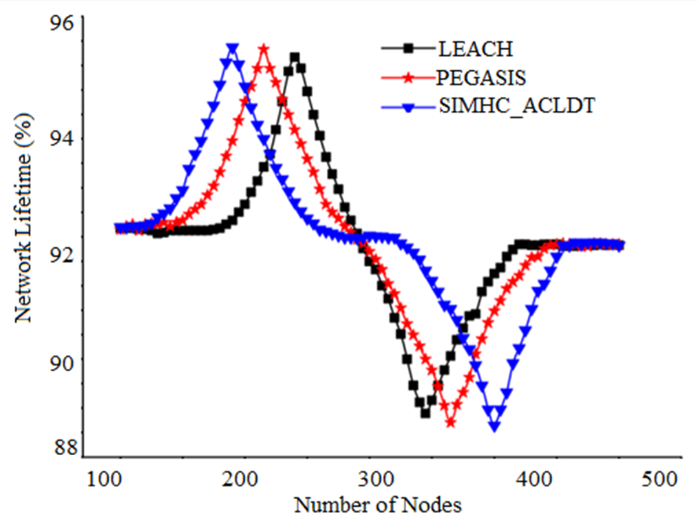
Network Lifetime (%)	94	95	96
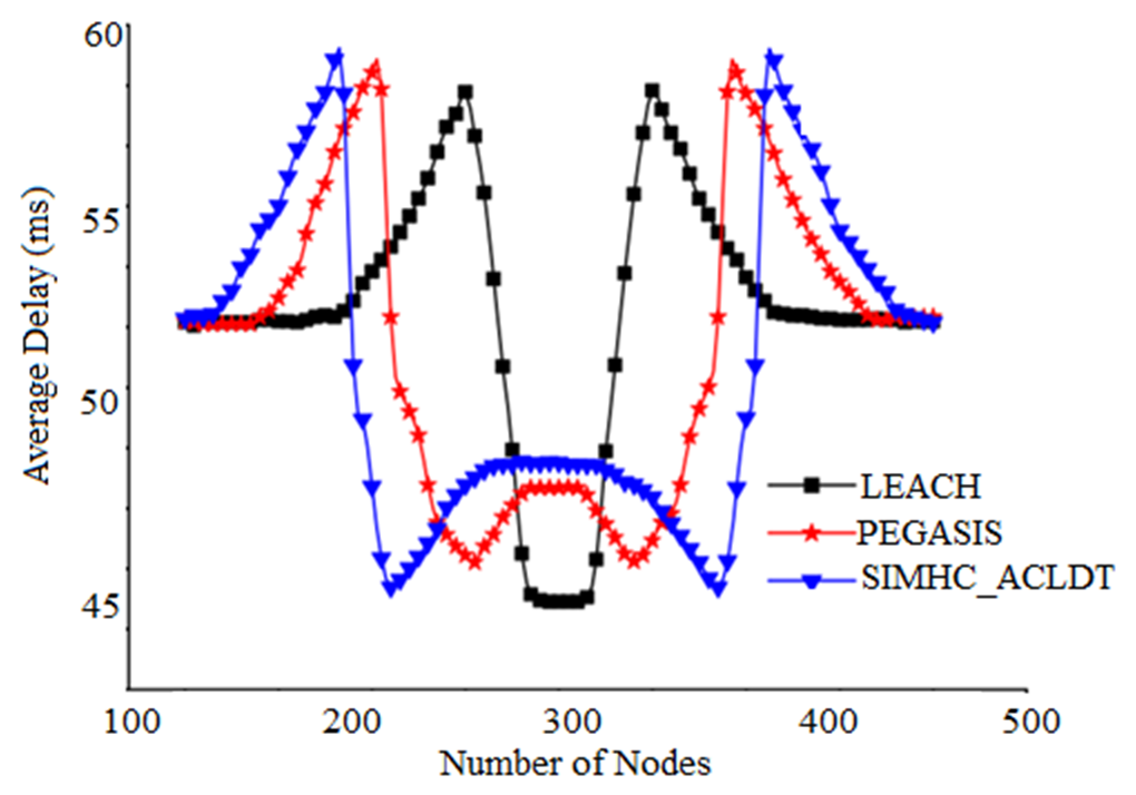
Average Delay (ms)	60	55	53
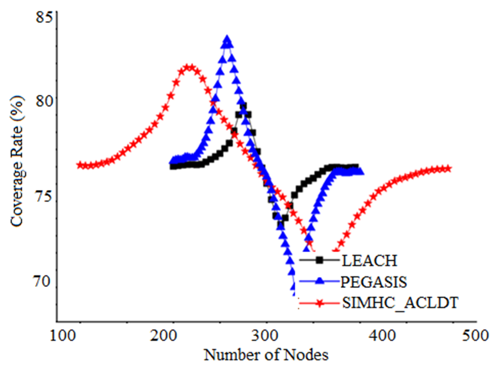
Coverage Rate (%)	75	78	83
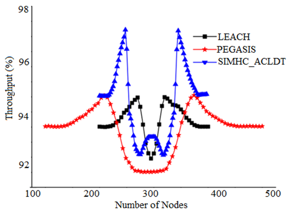
Throughput (%)	93	94	97
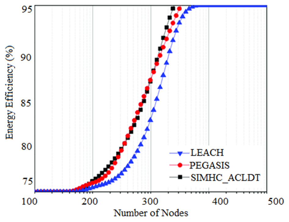
Energy Efficiency (%)	94	94.6	95

presents the comparative analysis of the proposed SIMHC_ACLDT with existing techniques, namely LEACH and PEGASIS, based on the network lifetime, average delay, coverage rate, throughput, and energy efficiency.

Figure 2, Figure 3, Figure 4, Figure 5 and Figure 6 present the comparative analysis results of the proposed SIMHC_ACLDT and existing LEACH and PEGASIS techniques. SIMHC_ACLDT obtained optimal results for clustering-based data transmission and low power consumption in the network. Specifically, the proposed method achieved a network lifetime of up to 96%, average delay of 53 ms, coverage rate of 83%, data transmission of 97%, and energy efficiency of 95%.

5. Conclusions

This work proposes a novel sensor-system-based network by integrating multi-hop communication with swarm intelligence to achieve low-power communication and data transmission. In this technique, clustering is combined with data transfer via location-based routing and low-power communication in two phases to calculate the ideal cluster heads (CHs). Initially, the nodes are clustered and calculated to determine the optimal CHs. Then, the data transmission is performed using the adaptive clustering-based locative data transmission (ACLDT) algorithm, where the sink node and base station locations are precisely known. A CH will seek the nearest CH and utilize it as the next hop, and then a path to the base station is formed through the development of CH chains. The experimental results show that this technique can attain a network lifetime of 96%, average delay of 53 ms, coverage rate (CR) of 83%, throughput of 97%, and an energy efficiency of 95%. In future works, this low power consumption model with efficient data transmission can be implemented and simulated in real-time applications, such as VANET integrated with cloud architecture to enhance network security.

References

- Shaheen, Q.; Shiraz, M.; Hashmi, M.U.; Mahmood, D.; Akhtar, R. A lightweight location-aware fog framework (LAFF) for QoS in the IoT paradigm. Mob. Inf. Syst. 2020, 2020, 8871976. [Google Scholar]
- Yao, B.; Gao, H.; Chen, Q.; Li, J. Energy-Adaptive and Bottleneck-Aware Many-to-Many Communication Scheduling for Battery-Free WSNs. IEEE Internet Things J. 2021, 8, 8514–8529. [Google Scholar] [CrossRef]
- Zhang, Z.; Li, J.; Yang, X. Data Aggregation in Heterogeneous Wireless Sensor Networks by using Local Tree Reconstruction Algorithm. Complexity 2020, 2020, 3594263. [Google Scholar] [CrossRef]
- Kim, T.; Vecchietti, L.F.; Choi, K.; Lee, S.; Har, D. Machine Learning for Advanced Wireless Sensor Networks: A Review. IEEE Sens. J. 2021, 21, 12379–12397. [Google Scholar] [CrossRef]
- Almaslukh, B. Deep Learning and Entity Embedding-Based Intrusion Detection Model for Wireless Sensor Networks. CMC Comput. Mater. Contin. 2021, 69, 1343–1360. [Google Scholar] [CrossRef]
- Karthik, S.S.; Kavithamani, A. Fog computing-based deep earning model for optimization of microgrid-connected WSN with load balancing. Wirel. Netw. 2021, 27, 2719–2727. [Google Scholar] [CrossRef]
- Zhou, Q.; Chen, Y.; Li, B.; Li, X.; Zhou, C.; Huang, J.; Hu, H. Training deep neural networks for wireless sensor networks using loosely and weakly labeled images. Neurocomputing 2021, 427, 64–73. [Google Scholar] [CrossRef]
- Wu, S.; Min, X.; Li, J. Optimal Data Transmission for WSNs with Data-Location Integration. Symmetry 2021, 13, 1499. [Google Scholar] [CrossRef]
- Shukry, S. Stable routing and energy-conserved data transmission over wireless sensor networks. EURASIP J. Wirel. Commun. Netw. 2021, 2021, 36. [Google Scholar] [CrossRef]
- Khan, M.K.; Shiraz, M.; Shaheen, Q.; Butt, S.A.; Akhtar, R.; Khan, M.A.; Changda, W. Hierarchical Routing Protocols for Wireless Sensor Networks: Functional and Performance Analysis. J. Sensors 2021, 2021, 7459368. [Google Scholar] [CrossRef]
- Abdurohman, M.; Supriadi, Y.; Fahmi, F.Z. A modified E-LEACH routing protocol for improving the lifetime of a wireless sensor network. J. Inf. Processing Syst. 2020, 16, 845–858. [Google Scholar]
- Chéour, R.; Jmal, M.W.; Khriji, S.; El Houssaini, D.; Trigona, C.; Abid, M.; Kanoun, O. Towards Hybrid Energy-Efficient Power Management in Wireless Sensor Networks. Sensors 2021, 22, 301. [Google Scholar] [CrossRef] [PubMed]
- Liu, X.; Wu, J. A method for energy balance and data transmission optimal routing in wireless sensor networks. Sensors 2019, 19, 13. [Google Scholar] [CrossRef] [PubMed] [Green Version]
- Ketshabetswe, L.K.; Zungeru, A.M.; Mangwala, M.; Chuma, J.M.; Sigweni, B. Communication protocols for wireless sensor networks: A survey and comparison. Heliyon 2019, 5, e01591. [Google Scholar] [CrossRef] [PubMed] [Green Version]
- Fathy, Y.; Barnaghi, P. Quality-Based and Energy-Efficient Data Communication for the Internet of Things Networks. IEEE Internet Things J. 2019, 6, 10318–10331. [Google Scholar] [CrossRef]
- Sefati, S.; Abdi, M.; Ghaffari, A. Cluster-based data transmission scheme in wireless sensor networks using black hole and ant colony algorithms. Int. J. Commun. Syst. 2021, 34, e4768. [Google Scholar] [CrossRef]
- Singh, M.K.; Amin, S.I. Energy-efficient data transmission technique for wireless sensor networks based on DSC and virtual MIMO. ETRI J. 2020, 42, 341–350. [Google Scholar] [CrossRef]
- Regin, R.; Rajest, S.; Singh, B. Fault Detection in Wireless Sensor Network Based on Deep Learning Algorithms. EAI Endorsed Trans. Scalable Inf. Syst. 2018, 21, e8. [Google Scholar] [CrossRef]
- Saban, M.; Medus, L.D.; Casans, S.; Aghzout, O.; Rosado, A. Sensor Node Network for Remote Moisture Measurement in Timber Based on Bluetooth Low Energy and Web-Based Monitoring System. Sensors 2021, 21, 491. [Google Scholar] [CrossRef]
- Fan, T.; Liu, Z.; Luo, Z.; Li, J.; Tian, X.; Chen, Y.; Feng, Y.; Wang, C.; Bi, H.; Li, X.; et al. Analog Sensing and Computing Systems with Low Power Consumption for Gesture Recognition. Adv. Intell. Syst. 2020, 3, 2000184. [Google Scholar] [CrossRef]
- Nurelmadina, N.; Hasan, M.; Memon, I.; Saeed, R.; Ariffin, K.Z.; Ali, E.; Mokhtar, R.; Islam, S.; Hossain, E.; Hassan, A. A Systematic Review on Cognitive Radio in Low Power Wide Area Network for Industrial IoT Applications. Sustainability 2021, 13, 338. [Google Scholar] [CrossRef]
- Yadav, A.; Kumar, S.; Vijendra, S. Network Life Time Analysis of WSNs Using Particle Swarm Optimization, International Conference on Computational Intelligence and Data Science (ICCIDS 2018). Procedia Comput. Sci. 2018, 132, 805–815. [Google Scholar] [CrossRef]