Optimization of Spatial Resolution and Image Reconstruction Parameters for the Small-Animal Metis™ PET/CT System

Abstract

Purpose: The aim of this study was to investigate the optimization of the spatial resolution and image reconstruction parameters related to image quality in an iterative reconstruction algorithm for the small-animal Metis™ PET/CT system. Methods: We used a homemade Derenzo phantom to evaluate the image quality using visual assessment, the signal-to-noise ratio, the contrast, the coefficient of variation, and the contrast-to-noise ratio of the 0.8 mm hot rods of eight slices in the center of the phantom PET images. A healthy mouse study was performed to analyze the influence of the optimal reconstruction parameters and the Gaussian post-filter FWHM. Results: In the phantom study, the image quality was the best when the phantom was placed at the end, keeping the central axis parallel to the X-axis of the system, and selecting between 30 and 40 iterations, a 0.314 mm reconstructed voxel size, and a 1.57 mm Gaussian post-filter FWHM. The optimization of the spatial resolution could reach 0.6 mm. In the animal study, it was suitable to choose a voxel size of 0.472 mm, between 30 and 40 iterations, and a 2.36 mm Gaussian post-filter FWHM. Conclusions: Our results indicate that the optimal imaging conditions and reconstruction parameters are very necessary to obtain high-resolution images and quantitative accuracy, especially for the high-precision recognition of tiny lesions.

1. Introduction

As a dual-modality medical imaging device, PET/CT is widely used in the diagnosis and treatment planning of diseases. High-resolution small-animal PET/CT plays an important role in preclinical studies because of its high sensitivity and resolution [1,2]. Since sensitivity and spatial resolution are an oxymoron, a trade-off is challenging to achieve and needs to be explored and studied in depth [3,4,5]. The National Electrical Manufacturers Association (NEMA) recommended the use of the unified standard NEMA NU 4-2008 for the performance evaluation of small-animal PET/CT equipment in 2008, specifying the use of low-activity ²²Na point sources for spatial resolution measurement and a filtered back projection (FBP) algorithm for image reconstruction [6].

The majority of the literature reports that FBP introduces star-like artifacts [7,8,9,10], and it is not as widely used as iterative reconstruction algorithms at present. Hallen et al. mentioned that a more obvious solution for measuring the spatial resolution of a system is to use the scanner’s built-in reconstruction method (usually an iterative reconstruction algorithm) to reconstruct the point source data, which artificially increases the spatial resolution despite its non-negativity and non-linearly constrained nature. Another option is to use a micro-Derenzo phantom instead of a low-activity point source and allow the use of the scanner’s built-in reconstruction method [10]. The use of Derenzo phantoms with different specifications as auxiliary experiments to evaluate the spatial resolution of a system is a common method used by many scholars [11,12,13,14].

The spatial resolution or image quality obtained using the iterative reconstruction algorithm is limited by the location and orientation of the phantom to be scanned, the accuracy of the system response matrix (SRM) modeling, the number of subsets and iterations of the reconstruction, the full width at half maximum (FWHM) of the Gaussian post-filter, and the reconstruction matrix and voxel size. Optimal image reconstruction parameters are necessary for small-animal PET/CT systems to improve spatial resolution and quantitative accuracy [15,16]. In this study, we determined the optimal imaging conditions and reconstruction parameters in terms of image quality and resolution through a homemade Derenzo phantom experiment. Then, we analyzed the impact of the optimal reconstruction parameters on PET imaging in animals.

2. Materials and Methods

2.1. System Description

The small-animal Metis™ PET/CT is a lutetium yttrium orthosilicate scintillation crystal (LYSO)-based advanced scanner dedicated to rodent imaging, which is produced by Shandong Madic Technology Co., Ltd. in China. As shown in Figure 1, the physical 3D coordinates of the scanner follow the right-hand rule. The scanner consists of 32 detector boxes arranged in 4 consecutive octagonal rings with an axial length of 122 mm and a ring diameter of 129 mm (effective imaging trans-axial FOV of 81 mm). Figure 2 shows a single detector box formed by coupling two crystal modules to a silicon photomultiplier (SiPM, HAMAMATSU S13361-3050NE-04) using a light guide. A metal–organic framework (MOF) exists for which the accurate selection of constituents can produce high thermal and chemical stability and crystals of ultrahigh porosity. It can be used for medical and biological applications, as well as for optoelectronic equipment [17]. Each crystal module consists of four 12 × 12 LYSO crystals (0.943 × 0.943 × 10 mm³ each). The crystal arrays containing the enhanced specular reflector (ESR) optical reflector film inside are placed on a 4 × 4 SiPM with the crystals centered at a distance of 1.028 mm. Gaps exist in the PET detection boxes, the crystal modules, and the crystal arrays, and the crystal sensitivity is self-normalized by interpolation to reduce the effect of noisy data [18]. The default energy window is 350–750 keV.

The system design integrates the scanning control operation and image processing software of the PET scanner into a single PC workstation. Collected data are stored in list mode, and image reconstruction is performed by the 3D ordered subsets expectation maximization (3D-OSEM) and the 3D maximum likelihood expectation maximization (3D-MLEM), which includes modular trigger dead time correction, coincidence system dead time correction, radionuclide decay correction, detection efficiency, and geometric normalization processing.

The image processing software includes two parts: image reconstruction and image analysis. Image reconstruction contains four different reconstruction settings, as shown in

Table 1. Four different reconstruction parameter settings.

	Matrix Size	Axial Slices	Isotropic Voxel Size (mm)
(1)	85 × 85	129 layers	0.943
(2)	128 × 128	194 layers	0.629
(3)	171 × 171	259 layers	0.472
(4)	257 × 257	389 layers	0.314

. The experiment operator can choose different reconstruction settings according to the acquisition protocol of different tissues or regions of interest (ROIs). Different manufacturers define different image data formats (defined as .mpv format in this study), which are generally packaged into a unified DICOM data format. Image analysis includes operations such as quantitative or semi-quantitative calculation of digital images, image smoothing and filtering, window width and level adjustment, delineation of ROIs, pharmacokinetics, and time–activity curves (TACs).

2.2. Reconstruction Algorithm and Parameters

Hudson and Larkin introduced the idea of ordered subsets to the maximum likelihood expectation maximization reconstruction algorithm in 1994 [19]. The basic principle of OSEM is to divide all projection data into S subsets, which are updated by several iterations to reach image convergence. The list-mode 3D-OSEM algorithm formula can be described as follows [20]:

$${\lambda }_j^{m,l}=\frac{{\lambda }_j^{m,l-1}}{N_j}{\displaystyle \sum _{k\in S_l}{p}_{i_{k}j}}\frac{A}{s_{i_k}+r_{i_k}+{\displaystyle \sum _{b=1}^J{p}_{i_{k}b}{\lambda }_b^{m,l-1}}},$$

(1)

where ${\lambda }_j^{m,l}$ represents the 3D reconstruction image after m iterations and l subsets, and the subscript index of the voxel is j = 1 … J; S_l indicates that the events are divided into S_l subsets, and the subscript l is the number of subsets; $p_{ij}$ is the probability that the j-th voxel produces a pair of gamma rays on the i-th response line (LOR); $s_{i_k}$ and $r_{i_k}$ are the scatter and random coincidence coefficients of the LOR where the i_k-th event is located, respectively; and A is the correction factor. The calculation formula is as follows:

$$A={\eta }_{Decay}{\eta }_{TrigDeadTime}{\eta }_{CoincidenceDeadTime},$$

(2)

where ${\eta }_{Decay}$ is the radionuclide decay correction coefficient, ${\eta }_{TrigDeadTime}$ is the crystal module trigger dead time correction coefficient, and ${\eta }_{CoincidenceDeadTime}$ is the coincidence system dead time correction coefficient.

$N_j$ refers to the sensitivity image of the system, including detector geometric efficiency and tissue attenuation. In fact, the calculation of the sensitivity image is to traverse all possible LORs, and for each LOR, its contribution to each voxel is calculated. The calculation formula is as follows:

$$N_j={\displaystyle \sum _{i=1}^L{\omega }_i{p}_{ij}},$$

(3)

where j is the voxel index, i represents the LOR, and L is the total number of LORs. ${\omega }_i$ indicates the normalized weight which contains two parts: one is the detector normalization factor ${\eta }_{Normalization}$ (including detection efficiency and spatial geometric efficiency), and the other is the attenuation correction coefficient ${\eta }_{Attenuation}$.

In this study, the double energy window method was mainly used for scatter coincidence correction. The random coincidence correction was accomplished by delaying the coincidence window to obtain random coincidence counts and subtracting these counts from the actual counts in real time. A Gaussian post-filter with an FWHM of 5 times the voxel size was used as a smoothing filter in all reconstruction models. Meanwhile, a tube of response (TOR) with a 5-fold voxel size was used in the reconstruction [20].

2.3. Derenzo Phantom Studies

A homemade micro-Derenzo phantom with hole diameters of 0.5, 0.6, 0.7, 0.8, 0.9, and 1.0 mm was used to measure the spatial resolution of the PET/CT system. The center-to-center distance between adjacent rods in the same group was twice the rod diameter. Figure 3 shows the end view of the micro-Derenzo phantom. The experiment of the phantom included six sub-experiments, with regard to injecting fluorine-18 (¹⁸F)-fluorodeoxyglucose (FDG) mixed with saline into the phantom and placing it at the end of the scanning bed or at the center of the PET FOV for data acquisition, as shown in

Table 2. The six sub-experiments in the measurement of the PET/CT system spatial resolution using a micro-Derenzo phantom.

Orientation	Position	Initial Activity (MBq)	Acquisition Time (min)	Reconstruction Algorithms
The central axis of the rods parallel to the Z-axis of the PET system	End (Ze) 1	3.45	20	OSEM/MLEM
	Center (Zc) 2	3.62	20	OSEM/MLEM
The central axis of the rods parallel to the Y-axis of the PET system	End (Ye)	3.71	20	OSEM/MLEM
	Center (Yc)	3.23	20	OSEM/MLEM
The central axis of the rods parallel to the X-axis of the PET system	End (Xe)	3.68	20	OSEM/MLEM
	Center (Xc)	3.74	20	OSEM/MLEM

¹ Ze means that the Derenzo phantom was placed at the end of the FOV, and the central axis of the rods was kept parallel to the Z-axis of the PET system. ² Zc means that the Derenzo phantom was placed at the center of the FOV, and the central axis of the rods was kept parallel to the Z-axis of the PET system. Similar for Ye, Yc, Xe, and Xc.

.

The collected data were reconstructed using the 3D-MLEM and 3D-OSEM algorithms, with the iterations ranging from 1 to 40, and the subsets ranging from 5 to 30 intervals. The voxel size was 0.314 mm, and the FWHM of the Gaussian post-filter was set to 5 times the voxel size. We determined the optimal reconstruction parameters to interpret the orientation and location of the phantom with the best image quality and resolution. Meanwhile, we compared the reconstruction speed of the best sub-experiment using the 3D-MLEM and 3D-OSEM algorithms.

For the sub-experiment with optimal imaging, we also evaluated the effect of the FWHM of the Gaussian post-filter on image quality using the 3D-MLEM reconstruction algorithm.

2.4. Data Analysis Methods

The purpose of data analysis was to evaluate the optimal image conditions and reconstruction parameters, including orientation, position, subsets, iterations, reconstructed voxel size, and Gaussian post-filter FWHM. The analysis of PET images of the Derenzo phantom was performed using visual assessment, the signal-to-noise ratio (SNR), the contrast, the coefficient of variation (CV), and the contrast-to-noise ratio (CNR) [21]. For the reconstructed PET images, we drew circular ROIs with a diameter of 0.8 mm in each 0.8 mm hot rod center of 8 slices in the center of the phantom. We also drew circular ROIs with a diameter of 1.6 mm in each 0.8 mm hot rod center as the background. The 8 slices in the center of the phantom need to be judged according to the different orientations and positions of the six sub-experiments.

For visual assessment, the PET images of the Derenzo phantom were evaluated against the smallest hot rods that can be clearly identified. The SNR, contrast, CV, and CNR of the 0.8 mm hot rods were used for the quantitative analysis of the Derenzo phantom. The SNR was calculated as follows:

$$SNR=S_{mean}/SD,$$

(4)

where $S_{mean}$ is the mean signal intensity of 0.8 mm ROIs in each 0.8 mm hot rod center of 8 slices in the center of the phantom, and $SD$ is the standard deviation of the background. The contrast, CV, and CNR of the 0.8 mm hot rods in the phantom images were calculated, respectively, as follows:

$$Contrast=S_{mean}/B_{mean},$$

(5)

$$CV=SD/B_{mean},$$

(6)

$$CNR=\left(S_{mean}-B_{mean}\right)/SD,$$

(7)

where $B_{mean}$ is the average intensity of the 1.6 mm background ROIs.

2.5. Animal Study

Animal studies were approved by the Laboratory Animal Ethics Committee of Xuzhou Medical University (Process number for animal experiments: 201706w010). A 40 g, 110 mm-long healthy mouse fasted in advance was injected with 18.58 MBq ¹⁸F-FDG via the tail vein after the induction of anesthesia, which used a mixture of oxygen (11/min) and isoflurane (1.5%). Seventy minutes after ingestion, we placed the mouse on the gantry along the Z-axis of the PET system for a 30 min whole-body static scan and continued to induce anesthesia. We used the optimal reconstruction parameters from the Derenzo phantom experiments to reconstruct the mouse raw data and observed the effect of the Gaussian post-filter FWHM on mouse imaging. All methods were carried out in accordance with relevant guidelines and regulations. This study was carried out in compliance with the ARRIVE guidelines.

3. Results

3.1. Derenzo Phantom Analysis

For the qualitative analysis of the Derenzo phantom, the main benchmark was all the hot rods in a group that could be clearly distinguished visually, as a way to determine the resolution of the image. For quantitative analysis of the Derenzo phantom, the larger the CNR value, the larger the contrast value, the smaller the CV value, and the larger the SNR value, the better the quality of the image.

Figure 4 shows the analysis of the PET image quality of the Derenzo phantom reconstructed by the system’s 3D-MLEM algorithm for different orientations and positions. PET images with the central axis of the rods parallel to Z-axis of the PET system (Zc, Ze) are not shown here, as they were very poorly visualized, and only 0.9 mm hot rods could be identified. As the 0.8 mm hot rods were not clearly visible in the PET images, the corresponding image quality analysis of Zc and Ze could not be performed.

The image quality of Xe in Figure 4 was the best, with a 0.6 mm hot rod visible. For Ye, Yc, and Xc, the smallest identifiable rods were 0.7 mm, 0.8 mm, and 0.8 mm, respectively. The SNR, contrast, CV, and CNR are plotted in Figure 5 as a function of the iteration number. In these experiments, the SNR values of Xc were the highest between 1 and 25 iterations, with a maximum at iteration 10, followed by Xe with a maximum at iteration 15. Xe, Xc, Ye, and Yc reached convergence roughly at iteration 25. For the contrast and CNR analysis, Xe had the highest contrast and CNR values, Xc had the lowest contrast and CNR values, and Ye and Yc had intermediate values. As the iterations increased, the CV of the images continued to increase. In all iterations, Xc’s image had the smallest CV value, with Ye being second to it.

Figure 6 shows the analysis of the PET image quality of the Derenzo phantom reconstructed with the 3D-OSEM algorithm (subset 5) in different orientations and positions. We also analyzed other PET images reconstructed with multiple subsets using the image quality evaluation metric. The images of Xe clearly identified 0.6 mm hot rods, followed by Xc and Ye, which identified 0.7 mm hot rods. Yc had the worst imaging, with only 0.8 mm hot rods visible. Meanwhile, the images from iterations 8 to 12 showed little change for the six sub-experiments from a visual assessment.

Figure 7 shows the change in image quality metrics as the number of iterations increased. In the image SNR analysis, Ye had the highest values in these experiments from iterations 4 to 20, followed by Yc. The SNR values of Yc, Xc, and Xe gradually converged and overlapped after 15 iterations. Xe and Xc reached convergence after approximately six iterations. Xe had the highest contrast values from iterations 1 to 12, the highest CNR values from iterations 1 to 7, and the highest CV values in all iterations, while Yc had the lowest contrast, CV, and CNR values across all iterations. Ye had the highest contrast values after 12 iterations and the highest CNR values after 7 iterations. The contrast and CNR values of Xc and Ye intersected at three iterations, and the CV values intersected at six iterations. The CV values under different imaging conditions increased with the number of iterations. Thus, the optimal imaging quality can be extrapolated to 6–12 iterations at a subset of 5. Qualitative and quantitative results for other multiple subsets of images show that the best images occurred at 10 subsets and 3 to 4 iterations, 15 subsets and 2 to 3 iterations, 20 subsets and 2 iterations, 25 subsets and 2 iterations, and 30 subsets and 1 iteration. Therefore, we can assume that the optimal resolution and image quality for the Derenzo phantom were at iterative updates (subsets × iterations) from 30 to 40.

Table 3. Time required for different iterative updates of the 3D-MLEM and 3D-OSEM (5 subsets) algorithms.

Iterative Updates	Time-3D-MLEM (s)	Time-3D-OSEM (s)	Ratio (%)
5	5	2	60
10	8	3	62.5
15	11	3	72.7
20	14	4	71.4
25	17	5	70.6
30	21	5	76.2
35	24	6	75
40	27	7	74.1

shows the time required for the two reconstruction algorithms. 3D-OSEM (subset 5) had an average reconstruction rate that was approximately 70.3% higher than that of 3D-MLEM. Figure 8 shows the effect of different Gaussian post-filter FWHMs on PET images of the Derenzo phantom using the 3D-MLEM algorithm (iteration 35). The image quality was visually the best when applying a Gaussian post-filter with a 1.57 mm FWHM, followed by a 2.36 mm FWHM.

3.2. Animal Analysis

The whole body of a mouse was imaged using the 3D-MLEM algorithm with an iteration update of 35 according to the optimal reconstruction parameters determined by the Derenzo phantom, as shown in Figure 9. The reconstructed voxel size of the PET image in Figure 9a was 0.472 mm, with a matrix size of 171 × 171, an axial slice of 259 layers, and an FWHM of 2.36 mm for the Gaussian post-filter. The reconstructed voxel size of the PET image in Figure 9b was 0.314 mm, the matrix size was 257 × 257, the axial slice was 389 layers, and the Gaussian post-filter FWHM was 1.57 mm. Comparing the coronal PET images of the mouse reconstructed by these two different reconstruction parameters, it can be clearly seen that the edges of tissue structures such as the brain, heart, and kidney of the mouse in Figure 9a are smooth, continuous, and low-noise, while in Figure 9b, they are discontinuous and uneven with artifacts. Although increasing the Gaussian post-filter FWHM can effectively reduce image noise, the local tissue details of the image become blurred. Therefore, the reconstruction parameters in Figure 9b can be selected when performing local precise quantitative imaging, such as on brain structures.

4. Discussion

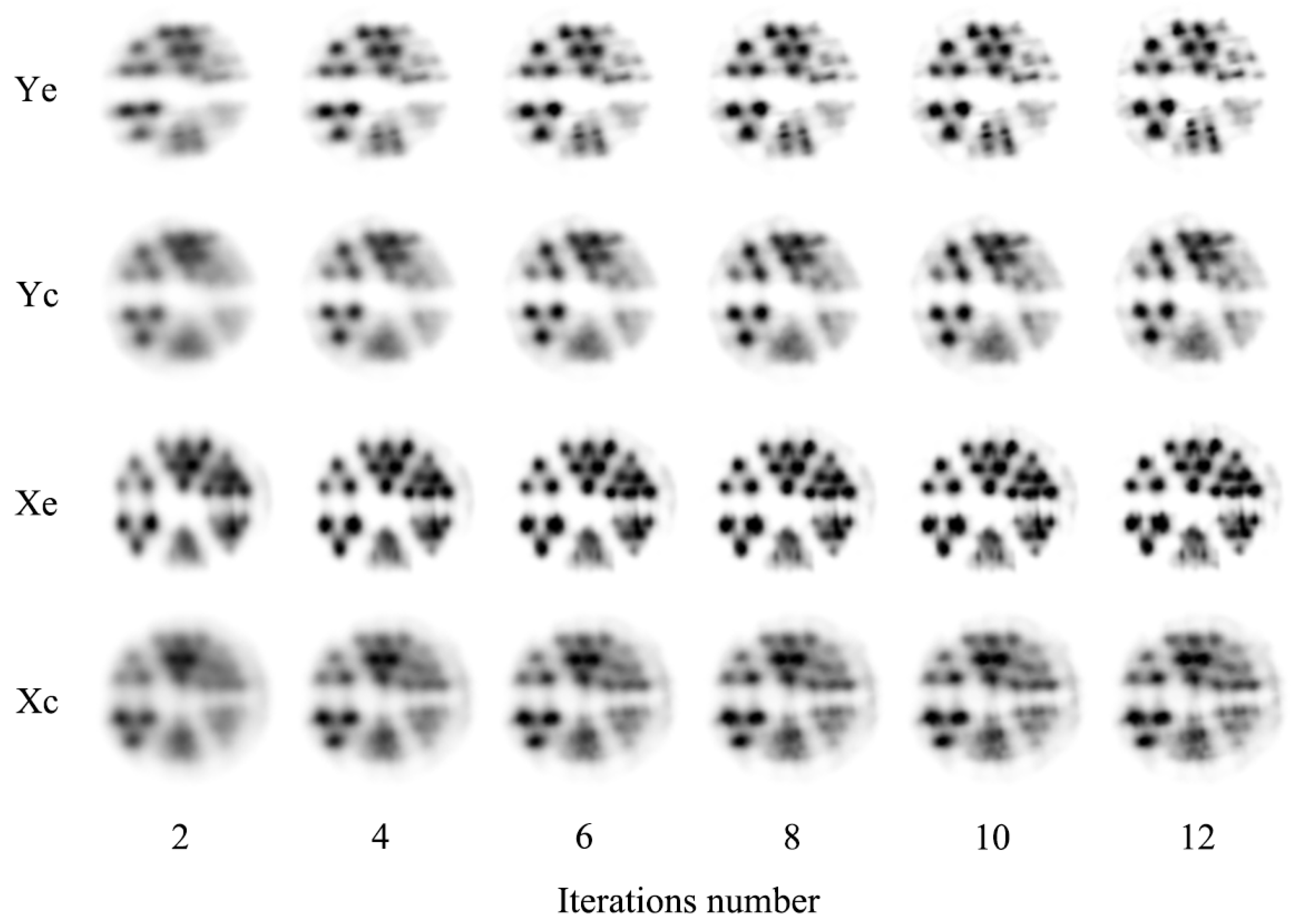
In this study, we evaluated the impact of different imaging conditions and reconstruction parameters in iterative reconstruction algorithms on PET image quality through micro-Derenzo phantom experiments, and investigated the optimization of the spatial resolution and image reconstruction parameters for the small-animal Metis™ PET/CT system. The PET image quality and spatial resolution were comprehensively analyzed through five image evaluation metrics: visual assessment, SNR, contrast, CV, and CNR. Our results show that the PET images gradually became clearer as the number of iterations increased, with the relevant evaluation metrics reaching convergence after 30 iterations. From the visual assessment analysis of Figure 4 and Figure 6, it can be found that placing the phantom at the end of the PET axial FOV and keeping the central axis of the rods parallel to the X-axis of the PET system result in the best image quality. We can clearly identify 0.6 mm hot rods. The PET images where the central axis of the rods was parallel to the Z-axis of the PET system (Zc, Ze) were very poorly visualized, and only 0.9 mm hot rods could be recognized. Additionally, the image quality of the Derenzo phantom placed at the end of the PET axial FOV was better than that placed at the center because the PET system has four detector rings and the center of the FOV has no detectors to receive gamma photons. We also found that the images from iterations 8 to 12 did not change much for the six sub-experiments, as shown by the visual assessment in Figure 6.

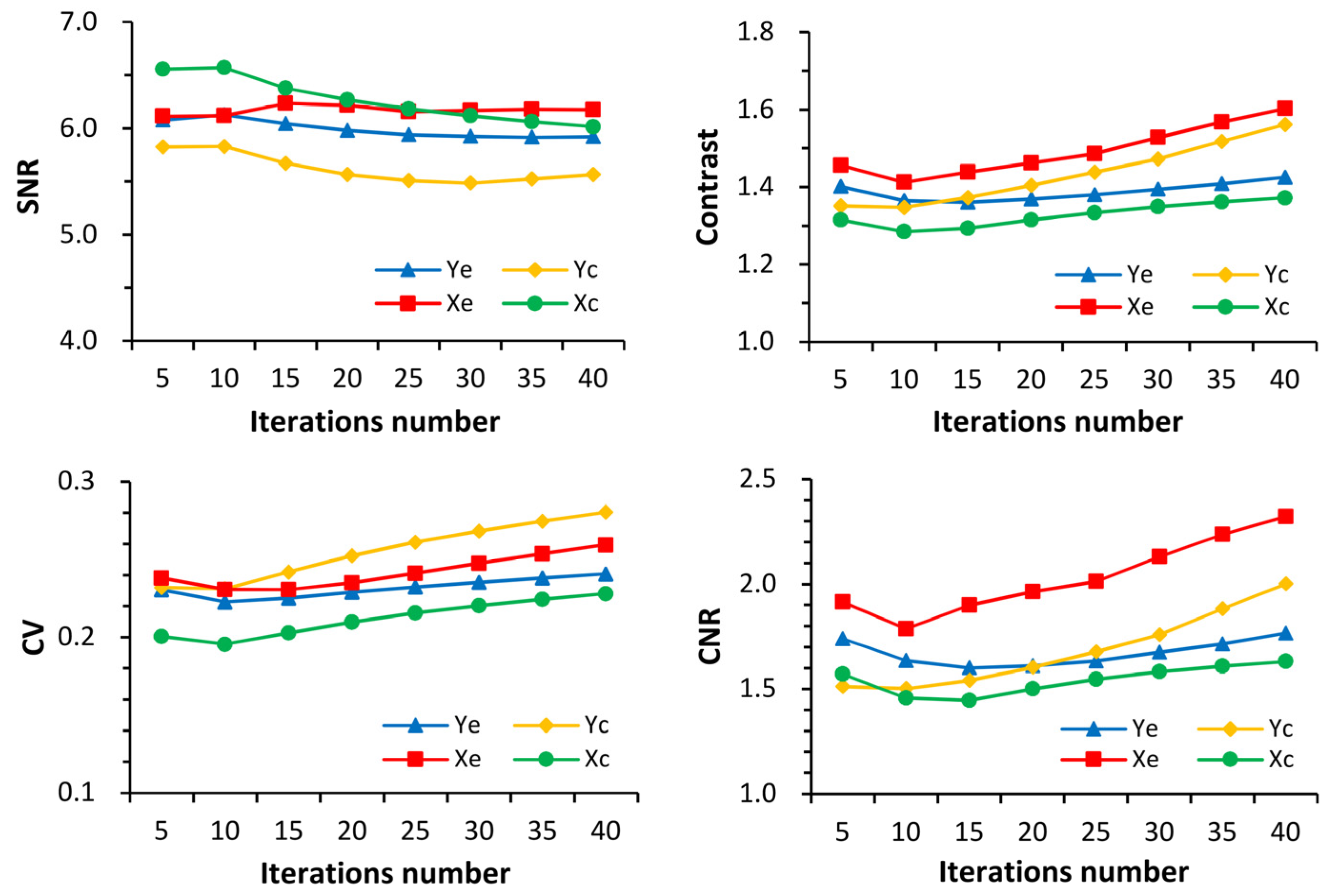
The SNR, CV, and contrast are mutually contradictory performance indicators, and the balance between them is affected by iterative updates. A trade-off needs to be found between them to achieve a high SNR, a high contrast, and a low CV [21]. As can be seen in Figure 5, the PET images of Xe had the highest SNR, contrast, and CNR values after 25 iterations, while Xc had the lowest contrast, CV, and CNR. Ye and Yc alternated with intermediate contrast and CNR values. Therefore, the optimal imaging conditions to evaluate the spatial resolution of the system by the Derenzo phantom would those for Xe, which is consistent with the results of the visual assessment, which suggests at least 25 iterations for a better image quality.

In Figure 7, Ye had the highest SNR values after four iterations, followed by Yc. The SNR values of Yc, Xc, and Xe gradually converged and overlapped after 15 iterations. Xe and Xc reached convergence at about six iterations. For the contrast, CV, and CNR analysis, Xe had the highest contrast values from iterations 1 to 12, the highest CV values in all iterations, and the highest CNR values from iterations 1 to 7, followed by Ye. In addition to the SNR, Xc and Yc showed similar trends in contrast, CV, and CNR analysis. For both the CV and CNR analyses, Xc and Ye and Xe and Ye intersected at approximately seven iterations. The results for other multiple subsets show that the best images appeared at 10 subsets and 3 to 4 iterations, 15 subsets and 2 to 3 iterations, 20 subsets and 2 iterations, 25 subsets and 2 iterations, and 30 subsets and 1 iteration. Based on the analysis of these experiments, the optimal number of iterations varied from 6 to 8 when the number of subsets was 5. Therefore, the product of the number of subsets and iterations between 30 and 40 is recommended for the optimal image quality.

We compared the reconstruction speed of the 3D-MLEM and 3D-OSEM algorithms for the Xe sub-experiment, as shown in Table 3. 3D-OSEM (subset 5) was, on average, nearly 70.3% faster than 3D-MLEM, but at the cost of increased image variance (noise level). For example, the CV values of each curve in Figure 7 were generally larger than those in Figure 5. Therefore, adjustments must be made in the selection of the optimal parameters for reconstruction. We also analyzed the effects of different reconstructed voxel sizes and Gaussian post-filter FWHMs on the image quality. Although increasing the Gaussian post-filter FWHM can effectively reduce image noise, the image became blurred and fewer hot rods could be identified [21,22]. When the reconstructed voxel size was 0.314 mm and the Gaussian post-filter FWHM was 1.57 mm, the image quality of the Derenzo phantom was the best, followed by a 2.36 mm FWHM. The image quality was the worst when the reconstructed voxel size was 0.943 mm and the Gaussian post-filter FWHM was 4.715 mm. Therefore, we chose 30 to 40 iterative updates, 0.472 mm and 0.314 mm reconstructed voxel sizes, and 1.57 mm and 2.36 mm Gaussian post-filter FWHMs to reconstruct the whole-body data of a healthy mouse.

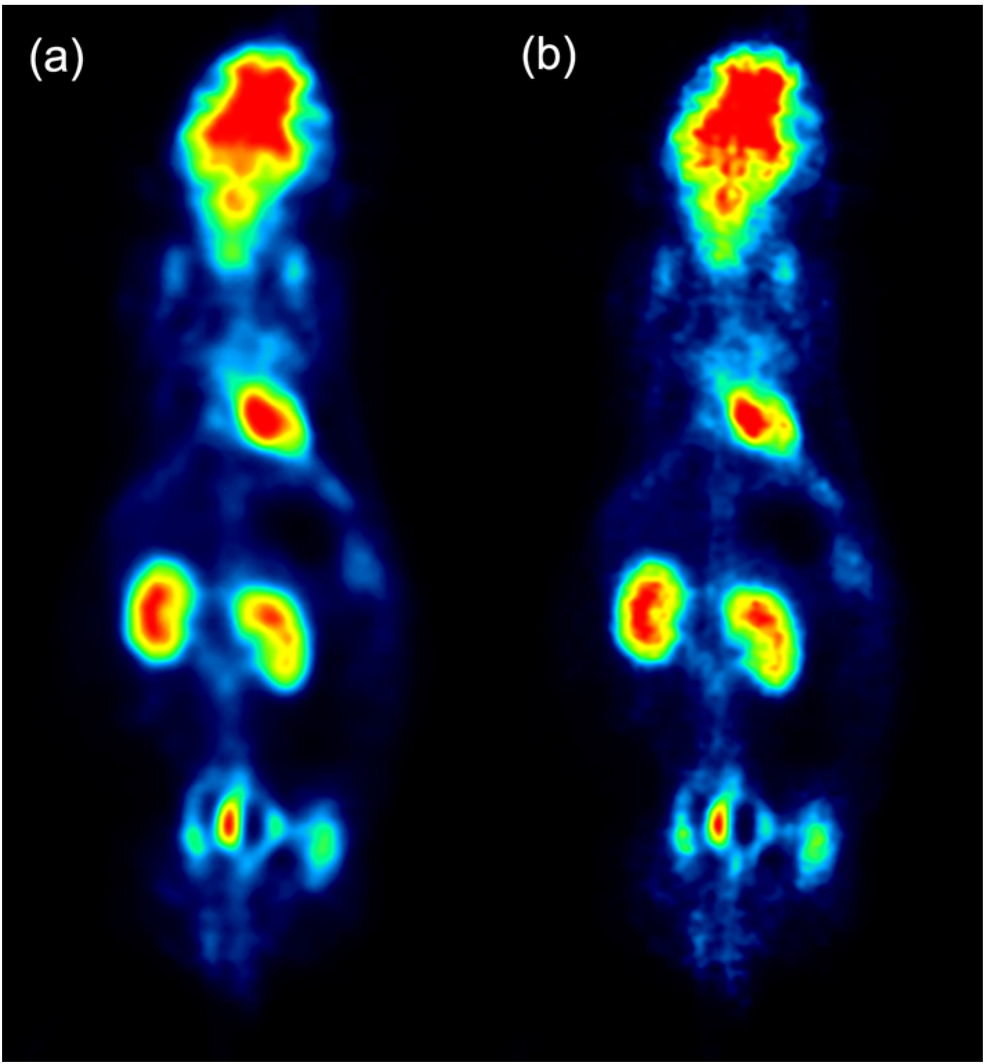
For the healthy mouse experiment, we mainly adopted the imaging method of Zc, as the effective trans-axial FOV of the PET system is 81 mm, which is smaller than the body length of the mouse. The smaller the voxel, the higher the accuracy, but a smaller voxel setting does not provide a better result. As can be seen in Figure 9a, when the reconstructed voxel size was 0.472 mm, the matrix size was 171 × 171, the axial slice was 259 layers, and the Gaussian post-filter FWHM was 2.36 mm, the edges of internal tissue structures such as the mouse brain, heart, and kidney were smooth and continuous. The image had significant contrast and no artifacts. However, the PET image in Figure 9b showed discontinuities, artifacts, and unevenness.

There are two limitations to consider in these analyses. First, the list-mode data of the Derenzo phantom were reconstructed by iterative algorithms under different imaging conditions to specifically evaluate the optimization of the spatial resolution and image reconstruction parameters for the small-animal Metis™ PET/CT system. The results of the evaluation are non-migrating and may not be applicable to other commercial small-animal PET systems, but the evaluation methods can be used as a reference. Secondly, we did not adequately consider the impact of the depth effect (DOI) on the spatial resolution of the system. Further investigation is required to perform accurate system modeling to improve the PET image quality and resolution.

5. Conclusions

Our results indicate that the optimal imaging conditions and reconstruction parameters are necessary to obtain high-resolution images and quantitative accuracy. In the phantom study, the best image quality was obtained by placing the Derenzo phantom at the end of the PET FOV, keeping the central axis of the phantom parallel to the X-axis of the PET system, and selecting between 30 and 40 iterative updates, a 0.314 mm reconstructed voxel size, and a 1.57 mm Gaussian post-filter FWHM. In the animal study, it was appropriate to choose a voxel size of 0.472 mm, between 30 and 40 iterative updates, and a 2.36 mm Gaussian post-filter FWHM for image reconstruction.

References

1. Yang, Y.; Bec, J.; Zhou, J.; Zhang, M.; Judenhofer, M.S.; Bai, X.; Di, K.; Wu, Y.; Rodriguez, M.; Dokhale, P.; et al. A Prototype High-Resolution Small-Animal PET Scanner Dedicated to Mouse Brain Imaging. J. Nucl. Med. 2016, 57, 1130–1135. [Google Scholar] [CrossRef] [PubMed] [Green Version]
2. Kuang, Z.; Wang, X.; Li, C.; Deng, X.; Feng, K.; Hu, Z.; Fu, X.; Ren, N.; Zhang, X.; Zheng, Y.; et al. Performance of a high-resolution depth encoding PET detector using barium sulfate reflector. Phys. Med. Biol. 2017, 62, 5945–5958. [Google Scholar] [CrossRef] [PubMed]
3. DiFilippo, F.P. Design of a Tri-PET collimator for high-resolution whole-body mouse imaging. Med. Phys. 2017, 44, 4230–4238. [Google Scholar] [CrossRef] [PubMed]
4. Daihong, J.; Sai, Z.; Lei, D.; Yueming, D. Multi-scale generative adversarial network for image super-resolution. Soft Comput. 2022, 26, 3631–3641. [Google Scholar] [CrossRef]
5. Liu, H.; Liu, J.; Hou, S.; Tao, T.; Han, J. Perception consistency ultrasound image super-resolution via self-supervised CycleGAN. Neural Comput. Appl. 2021, 8, 1–11. [Google Scholar] [CrossRef]
6. National Electrical Manufacturers Association. Performance Measurements of Small Animal Positron Emission Tomographs; Rosslyn, V.A., Ed.; NEMA Standards Publication NU 4–2008; National Electrical Manufacturers Association: Arlington, VA, USA, 2008. [Google Scholar]
7. Oda, K.; Toyama, H.; Uemura, K.; Ikoma, Y.; Kimura, Y.; Senda, M. Comparison of parametric FBP and OS-EM reconstruction algorithm images for PET dynamic study. Ann. Nucl. Med. 2001, 15, 417–423. [Google Scholar] [CrossRef] [PubMed]
8. Frese, T.; Rouze, N.C.; Bouman, C.A.; Sauer, K.; Hutchins, G.D. Quantitative comparison of FBP, EM, and Bayesian reconstruction algorithms for the IndyPET scanner. IEEE Trans. Med. Imaging 2003, 22, 258–276. [Google Scholar] [CrossRef] [PubMed]
9. Yu, A.R.; Kim, J.S.; Kang, J.H.; Lim, S.M. Comparison of reconstruction methods and quantitative accuracy in Siemens Inveon PET scanner. J. Instrum. 2015, 10, P04001. [Google Scholar] [CrossRef]
10. Hallen, P.; Schug, D.; Schulz, V. Comments on the NEMA NU 4-2008 Standard on Performance Measurement of Small Animal Positron Emission Tomographs. EJNMMI Phys. 2020, 7, 1300–1309. [Google Scholar] [CrossRef] [PubMed]
11. Nagy, K.; Tóth, M.; Major, P.; Patay, G.; Egri, G.; Häggkvist, J.; Varrone, A.; Farde, L.; Halldin, C.; Gulyás, B. Performance Evaluation of the Small-Animal nanoScan PET/MRI System. J. Nucl. Med. 2013, 54, 1825–1832. [Google Scholar] [CrossRef] [PubMed] [Green Version]
12. Gaudin, E.; Toussaint, M.; Thibaudeau, C.; Paille, M.; Fontaine, R.; Lecomte, R. Performance Simulation of an Ultrahigh Resolution Brain PET Scanner Using 1.2-mm Pixel Detectors. IEEE Trans. Radiat. Plasma Med. Sci. 2018, 3, 334–342. [Google Scholar] [CrossRef] [PubMed]
13. Pan, T.; Einstein, S.A.; Kappadath, S.C.; Grogg, K.S.; Gomez, C.L.; Alessio, A.M.; Hunter, W.C.; El Fakhri, G.; Kinahan, P.; Mawlawi, O.R. Performance evaluation of the 5-Ring GE Discovery MI PET/CT system using the national electrical manufacturers association NU 2-2012 Standard. Med. Phys. 2019, 46, 3025–3033. [Google Scholar] [CrossRef] [PubMed]
14. Sarnyai, Z.; Nagy, K.; Patay, G.; Molnár, M.; Rosenqvist, G.; Tóth, M.; Takano, A.; Gulyás, B.; Major, P.; Halldin, C.; et al. Performance Evaluation of a High-Resolution Nonhuman Primate PET/CT System. J. Nucl. Med. 2019, 60, 1818–1824. [Google Scholar] [CrossRef] [PubMed]
15. Shekari, M.; Ghafarian, P.; Ahangari, S.; Ghadiri, H.; Bakhshayeshkaram, M.; Ay, M.R. Optimizing Image Reconstruction Parameters in Time of Flight PET/CT Imaging: A Phantom Study. Front. Biomed. Technol. 2015, 2, 146–154. [Google Scholar]
16. Gaitanis, A.; Kastis, G.A.; Vlastou, E.; Bouziotis, P.; Verginis, P.; Anagnostopoulos, C.D. Investigation of Image Reconstruction Parameters of the Mediso nanoScan PC Small-Animal PET/CT Scanner for Two Different Positron Emitters under NEMA NU 4-2008 Standards. Mol. Imaging Biol. 2016, 19, 550–559. [Google Scholar] [CrossRef] [PubMed]
17. Safaei, M.; Foroughi, M.M.; Ebrahimpour, N.; Jahani, S.; Omidi, A.; Khatami, M. A review on metal-organic frameworks: Synthesis and applications. Trends Anal. Chem. 2019, 118, 401–425. [Google Scholar] [CrossRef]
18. Baghaei, H.; Zhang, Y.; Yan, H.; Wong, W.H. Evaluation of a self-normalization method for two PET cameras using prompt, delay or total emission data. In Proceedings of the Nuclear Science Symposium & Medical Imaging Conference 2016, Atlanta, GA, USA, 21–28 October 2017. [Google Scholar] [CrossRef]
19. Hudson, H.M.; Larkin, R.S. Accelerated image reconstruction using ordered subsets of projection data. IEEE Trans. Med. Imaging 1994, 13, 601–609. [Google Scholar] [CrossRef] [PubMed] [Green Version]
20. Pratx, G.; Chinn, G.; Olcott, P.D.; Levin, C.S. Fast, Accurate and Shift-Varying Line Projections for Iterative Reconstruction Using the GPU. IEEE Trans. Med. Imaging 2008, 28, 435–445. [Google Scholar] [CrossRef] [PubMed] [Green Version]
21. Akamatsu, G.; Ishikawa, K.; Mitsumoto, K.; Taniguchi, T.; Ohya, N.; Baba, S.; Abe, K.; Sasaki, M. Improvement in PET/CT Image Quality with a Combination of Point-Spread Function and Time-of-Flight in Relation to Reconstruction Parameters. J. Nucl. Med. 2012, 53, 1716–1722. [Google Scholar] [CrossRef] [PubMed] [Green Version]
22. Yoon, H.J.; Jeong, Y.J.; Son, H.J.; Kang, D.-Y.; Hyun, K.-Y.; Lee, M.-K. Optimization of the spatial resolution for the GE discovery PET/CT 710 by using NEMA NU 2-2007 standards. J. Korean Phys. Soc. 2015, 66, 287–294. [Google Scholar] [CrossRef]
Figure 1. Small-animal Metis™ PET/CT system.
Electronics 11 01542 g001
Figure 2. The internal view of a PET detector box, which contains two crystal modules, and each crystal module contains four crystal arrays.
Electronics 11 01542 g002
Figure 3. Photograph of the micro-Derenzo phantom (end view). The sizes of the porous arrays in the counterclockwise orientation from small to large are 0.5, 0.6, 0.7, 0.8, 0.9, and 1.0 mm. The center-to-center distance between adjacent rods is twice the rod diameter.
Electronics 11 01542 g003
Figure 4. The PET images of the Derenzo phantom reconstructed by the 3D-MLEM (iteration 40) algorithm in different orientations and positions, and at different iteration numbers.
Electronics 11 01542 g004
Figure 5. The SNR, contrast, CV, and CNR of PET images reconstructed by the MLEM algorithm in different orientations and positions are plotted as a function of the iteration number.
Electronics 11 01542 g005
Figure 6. The PET images of the Derenzo phantom reconstructed by the 3D-OSEM algorithm (5 subsets, 20 iterations) in different orientations and positions, and at different iteration numbers.
Electronics 11 01542 g006
Figure 7. The SNR, contrast, CV, and CNR of PET images reconstructed by the 3D-OSEM algorithm (5 subsets, 20 iterations) in different orientations and positions are plotted as a function of the iteration number.
Electronics 11 01542 g007
Figure 8. The PET images of the Derenzo phantom of the Xe sub-experiment using the 3D-MLEM algorithm (iteration 35) with different Gaussian post-filter FWHMs.
Electronics 11 01542 g008
Figure 9. Whole-body PET imaging of a healthy mouse. (a) The reconstructed voxel size was 0.472 mm, and the Gaussian post-filter FWHM was 2.36 mm. (b) The reconstructed voxel size was 0.314 mm, and the Gaussian post-filter FWHM was 1.57 mm.
Electronics 11 01542 g009