Abstract
This paper proposes a novel architecture for the computation of XY-like functions based on the QH CORDIC (Quadruple-Step-Ahead Hyperbolic Coordinate Rotation Digital Computer) methodology. The proposed architecture converts direct computing of function XY to logarithm, multiplication, and exponent operations. The QH CORDIC methodology is a parallel variant of the traditional CORDIC algorithm. Traditional CORDIC suffers from long latency and large area, while the QH CORDIC has much lower latency. The computation of functions lnx and ex is accomplished with the QH CORDIC. To solve the problem of the limited range of convergence of the QH CORDIC, this paper employs two specific techniques to enlarge the range of convergence for functions lnx and ex, making it possible to deal with high-precision floating-point inputs. Hardware modeling of function XY using the QH CORDIC is plotted in this paper. Under the TSMC 65 nm standard cell library, this paper designs and synthesizes a reference circuit. The ASIC implementation results show that the proposed architecture has 30 more orders of magnitude of maximum relative error and average relative error than the state-of-the-art. On top of that, the proposed architecture is also superior to the state-of-the-art in terms of latency, word length and energy efficiency (power × latency × period /efficient bits).
1. Introduction
XY-like functions usually find their place in engineering and scientific applications such as digital signal processing, real-time 3D (three dimensions) graphics, scientific computing and so forth [1]. Currently, customized hardware designs for XY-like functions are becoming more promising due to the demanding timing constraints of these applications [2].
For most scientific applications, 64-bit floating-point (FP) numbers conforming to the IEEE-754(2008) standard are extensively applied. However, a rapidly growing number of scientific applications such as climate modeling, fluid mechanics, and economic analysis require a higher level of numerical precision [3]. This means that hundreds or more digits, such as 128 bits, are needed to gain valid numerical results.
Since XY = eYlnX, the computation of function XY can be decomposed into the logarithmic computation of lnX, the multiplication of lnX and Y, and the exponential computation eYlnX. Therefore, the computation of XY-like functions can be converted to the computation of logarithmic and exponential functions. The hardware methods of computing XY-like functions directly or indirectly can be divided into four categories: digit-recurrence [4,5,6], functional iteration [7,8,9], LUT (Look-Up Table)-based [10,11,12], and CORDIC-based [13,14,15]. In fact, CORDIC is one of the digit-recurrence algorithms.
The LUT method is simple and convenient, since look-up tables give the stored data according to their address index. Chen et al. [12] proposed a symmetric-mapping LUT-based method and an architecture to directly compute XY-like functions. The size of LUTs has a linear relation with the word length of address indexes and an exponential relation with the word length of storage data. It can be seen that the LUT method performs well in the case of low precision. However, as the precision of inputs increases, the size of LUTs expands dramatically. Under the requirement of high-precision inputs such as 128-bit FP inputs, the size of LUTs seems obviously unreasonable.
The functional iteration method usually computes eYlnX or 2Ylog2X indirectly instead of computing XY-like functions directly. Its principle is to transform logarithms and exponentials into a sum of a series of power exponents. Refs. [16,17,18,19] evaluate binary logarithms and exponentials via simple piecewise linear approximation. The main shortcoming of a simple linear approximation method is the high relative error with limited lookup tables. Paul et al. [20] use a second-order polynomial approximation method to reduce the relative error. In addition to binary logarithms and exponentials, a piecewise polynomial approximation for natural logarithms and exponentials is presented in [21]. To approximate natural logarithms and exponentials, Langhammer and Pasca [9] adopt a third-order piecewise Taylor expansion approximation method, which yields a faster processing speed than in [21]. All the functional iteration methods above require LUTs. LUTs of larger size contribute to higher computing precision. However, the improvement of calculation precision calls for more terms of power exponents and more LUTs with much larger sizes, which leads to an increase in both the computing complexity and timing latency. Therefore, the functional iteration method is likewise not suitable for XY-like functions with high-precision inputs.
Compared with the LUT and functional iteration methods, the digit-recurrence method is more suitable for hardware implementation of XY-like functions with wide word length. The characteristics of digit recurrence are bit-by-bit approximation and repeated calculation, which can be concisely constructed with logical and control blocks. The precision of the digit-recurrence method increases with the number of iterations. Pineiro et al. [4] exploits this method with high-radix arithmetic units to reduce the number of iterations when extracting binary logarithms and exponentials. Today, many commercial applications demand decimal floating-point arithmetic units. Therefore, Chen et al. [22,23] propose architectures for decimal logarithms and exponentials using the digit-recurrence method.
There are many kinds of digit-recurrence methods, including the CORDIC algorithm, the Gold–Schmidt (GS) iteration method, the Newton–Raphson (NR) iteration method, and so on. The convergence speed of GS iteration depends on the precision of the seed values corresponding to inputs. LUTs employed in Gold-Schmidt iteration to store seed values will expand sharply for high-precision inputs, with a similar effect on timing latency. The NR iteration method requires an initial guess, which may result in different precisions in the outputs [24,25,26]. The hardware complexity of the NR method increases with the increasing value of N.
Contrary to GS and NR iterations, the CORDIC algorithm is simple to implement, only includes shift and addition operations, and has a stable convergence speed and relatively fixed sizes of LUTs. Therefore, the CORDIC algorithm is widely used in the realization of transcendental functions.
The majority of CORDIC architectures for computing XY-like functions are based on the hyperbolic CORDIC algorithm. Traditional hyperbolic CORDIC suffers from high latency, large circuit area, and costly power consumption for the sake of its linear convergence speed.
In the latest literatures, Mack et al. [27] proposed an expanded hyperbolic CORDIC algorithm to compute powering functions for any FP number. Mopuri and Acharyya [14] did work on Nth power computations based on the binary hyperbolic CORDIC, which is a special case of the generalized hyperbolic CORDIC [13]. Luo et al. [28] employed the generalized hyperbolic CORDIC to directly compute logarithms and exponentials with an arbitrary fixed base.
However, there is not much research on general computation for XY-like functions with high-precision FP inputs. Such a generic approach for Nth power computation is proposed in [1] based on the natural logarithm–exponent relation, i.e., XY = eYlnX.
Duprat and Muller [29] introduced the Branching CORDIC algorithm, which enables a fast implementation of the CORDIC algorithm by performing two basic CORDIC rotations in parallel in two separate modules. D.S. Phatak [30] has improved the algorithm and proposed a double step branching CORDIC algorithm where two circular mode rotations are performed in a single step with little additional hardware. To achieve the goal of high-precision, high-accuracy, and low-latency in computing XY-like functions, this paper adopts the QH CORDIC methodology [31], which is inspired by the double step branching CORDIC algorithm. In this paper,
- We propose a parallel computing architecture with low-latency based on the QH CORDIC methodology;
- We enlarge the feasible range of FP inputs of the proposed architecture with specific techniques to make sure the proposed architecture applies to high-precision computing;
- We conduct hardware modeling on the proposed architecture to achieve the lowest possible circuit complexity and resource consumption;
- We compare the hardware implementation results with related works to show the minor-error and high-accuracy features of the proposed architecture.
The rest of this paper is organized as follows. Section 2 provides the necessary theoretical background of the QH CORDIC methodology. Section 3 introduces the hardware modeling of XY-like functions for 128-bit FP numbers. Section 4 shows the ASIC implementation results of the proposed architecture and compares it with the state-of-the-art in terms of correctness, word length, timing, and power. Section 5 concludes this paper.
2. QH CORDIC-Based Methodology of XY-Like Functions
In Section 2, emphasis is placed on the feasibility of logarithmic function lnx and exponential function ex computing with the QH CORDIC methodology.
We first review the QH CORDIC methodology in terms of iterative formulae. Then, we discuss the range of convergence (ROC) of the QH CORDIC methodology. Given the ROC of the QH CORDIC, the validity of computing of logarithmic function lnx and exponential function ex based on the QH CORDIC is analyzed.
2.1. Iterative Formulae of QH CORDIC Methodology
Based on shift-addition and vector rotation, the hyperbolic CORDIC algorithm is simple and efficient. However, hyperbolic CORDIC only generates one accurate bit per iteration, which is an apparent drawback for real-time scientific computing. Unlike traditional hyperbolic CORDIC, the QH CORDIC methodology combinates four sequential iterations into a single integrated iteration, greatly cutting down the quantity of iterations.
The iterative formulae of hyperbolic CORDIC are shown in Equation (1):
where σ is the rotation direction of the n-th rotation, θn = tanh−1(2−n), and n starts from 1.
Accordingly, the iterative formulae of the QH CORDIC are shown in Equation (2):
where σn, σn+1, σn+2, and σn+3 are rotation directions of the n-th, (n + 1)-th, (n + 2)-th, and (n + 3)-th rotations; θn = tanh−1(2−n), θn+1 = tanh−1[2−(n+1)], θn+2 = tanh−1[2−(n+2)], and θn+3 = tanh−1[2−(n+3)]; and n starts from 1.
The key of the QH CORDIC lies in the prediction of σ in four sequential steps, which is also the necklace of traditional hyperbolic CORDIC. In basic hyperbolic CORDIC, the value of σ is either −1 (rotating in a clockwise direction) or 1 (rotating in a counterclockwise direction). For a group of four sequential steps, the corresponding {σn, σn+1, σn+2, σn+3} has 16 possible cases for its values, from {−1, −1, −1, −1} to {1, 1, 1, 1}.
Substitute the 16 possible cases of {σn, σn+1, σn+2, σn+3} into (2) and obtain the 16 corresponding simplified expressions for xn+4, yn+4 and zn+4. Table 1 details the corresponding iterative formulae of yn+4 when {σn, σn+1, σn+2, σn+3} ranges from {−1, −1, −1, −1} to {1, 1, 1, 1}. Since the corresponding iterative formulae of xn+4 are almost the same as those of yn+4, a table that lists the iterative formulae of xn+4 is omitted.

Table 1.
Corresponding iterative formula of yn+4.
Table 2 details the corresponding iterative formulae of zn+4 when {σn, σn+1, σn+2, σn+3} ranges from {−1, −1, −1, −1} to {1, 1, 1, 1}.
Table 2.
Corresponding iterative formula of zn+4.
For an iteration step of the QH CORDIC in vectoring mode, parallelly compute 16 iterative formulae of yn+4 shown in Table 1 and obtain a group of 16 different values. Sort the closest-to-zero value out from the 16 yn+4 values and take it as the output of yn+4 in the current iteration step of the QH CORDIC. Simultaneously, take {σn, σn+1, σn+2, σn+3} corresponding to the iterative formula of the output of yn+4 as rotation directions in the current iteration step. Then, the computer outputs xn+4 and zn+4 with the iterative formulae of xn+4 and zn+4 corresponding to the rotation directions, respectively.
For an iteration step of the QH CORDIC in rotating mode, parallelly compute 16 iterative formulae of zn+4 shown in Table 2 and obtain a group of 16 different values. Sort the closest-to-zero value out from the 16 zn+4 values and take it as the output of zn+4 in the current iteration step of the QH CORDIC. Simultaneously, take {σn, σn+1, σn+2, σn+3} corresponding to the iterative formula of the output of zn+4 as the rotation directions in the current iteration step. Then, the computer outputs xn+4 and yn+4 with the iterative formulae of xn+4 and yn+4 corresponding to the rotation directions, respectively.
It can be seen in Table 1 that the eight upper iterative formulae of yn+4 (Cases 1–8) are partly symmetric to the eight lower iterative formulae (Cases 9–16). Such elaborate symmetry also exists with the iterative formulae of xn+4. To reduce the computational burden for every iteration step of the QH CORDIC, multiplications with the same absolute value of the coefficients can be simplified. By merging repeated multiplications into one multiplication and one sign-inversing operation, it takes 34 additions, 12 multiplications, and four shifts to parallelly finish the computation of the 16 iterative formulae of yn+4 shown in Table 1. Similarly, it takes 34 additions, 12 multiplications, and four shifts to parallelly finish the computation of the 16 iterative formulae of xn+4.
2.2. Range of Convergence of QH CORDIC Methodology
The ROCs of traditional hyperbolic CORDIC [32] are showed in Equation (3):
where y1 and x1 are initial inputs. It can be inferred that the angle of an input vector in radians for traditional hyperbolic CORDIC must be located in (−1.1182, 1.1182).
Similar to traditional hyperbolic CORDIC, constraints on the ROC of the QH CORDIC also exist.
Since the logarithmic function lnu cannot be attained directly by the QH CORDIC, the computation of function lnu is done through Equation (4):
The initial conditions and terminated statuses for QH CORDIC-based computation of lnu are listed in Equations (5) and (6), respectively:
Accompanied by Equation (3), the ROC of input u for function lnu is (0.11, 9.51).
As for the exponential function ev, the computation of function ev is done through Equation (7):
The initial conditions and terminated statuses for QH CORDIC-based computation of ev are listed in Equations (8) and (9), respectively:
According to Equation (3), the ROC of input v for function ev is (−1.1182, 1.1182).
Furthermore, when iteration times come to be 4, 13, 40, 121, ···, (3i+2 − 1)/2, ··· where i starts from 0, repeated iterations are necessary in order to ensure the convergence of the QH CORDIC [33]. In this manner, the actual sequence of iteration times of the QH CORDIC is 1, 2, 3, 4, 4, 5, ···, 12, 13, 13, ···.
2.3. Validity of Computation for Logarithmic Function and Exponential Function with QH CORDIC
As XY = eYlnX, it is necessary to study the validity of the computation for logarithmic function lnu and exponential function ev with the QH CORDIC, that is to say, to enlarge ROC of the QH CORDIC for logarithmic and exponential functions.
Since the inputs of the proposed architecture for XY-like functions are all FP numbers, suppose that the input FP number u is (−1)S × M × 2E, where S is sign of u, E is the exponent of u after correcting bias, M is the mantissa of u after complementing the implicit bit, and M ∈ [1, 2).
There is nothing ambiguous about S = 0 because the input FP number u for the logarithmic function lnu is bound to be positive. So, we obtain u = M × 2E. Perform natural logarithmic computation of both sides of u = M × 2E to obtain
To adjust M into the range of (0.11, 9.51), right-shift M one bit. Represent the right-shifted M as M′. Equation (10) is updated as
From Equation (11) we can see that the computation of lnu can be split into one logarithmic operation and one constant multiplication, as well as one addition.
In a similar way, the validity of the computation for exponential function ev with the QH CORDIC can also be ensured [15].
3. Hardware Modeling of XY-Like Functions with QH CORDIC
The QH CORDIC can be applied to both fixed-point and FP operations. Based on the QH CORDIC, this paper presents a quad-precision (128 bits) FP hardware modeling of XY-like functions.
The overall architecture of the quad-precision FP XY-like functions is illustrated in Figure 1. The proposed architecture is divided into three parts. As for XY-like functions, X is base while Y is index. Inputs are two quad-precision FP numbers: base and index (X and Y) and two control signals: clk and rst_n. Outputs are power_result and finish, which are a 128-bit calculated result of function XY and a completed signal of function XY, respectively. There are three segments in the overall hardware architecture for XY-like functions, the preprocessing module, the QH module, and the postprocessing module.
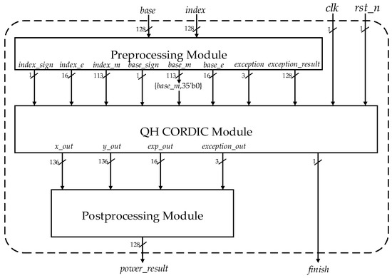
Figure 1.
Overall architecture of quad-precision FP XY-like functions.
3.1. Preprocessing Module
The preprocessing module judges whether exception situations exist after breaking down the two FP inputs base and index into three portions: sign (base_sign and index_sign), exponent (base_e and index_e) and mantissa (base_m and index_m). The program flowchart of the preprocessing module is presented in Figure 2. As it is shown in Figure 2, for the quad-precision FP input base, base_sign is a 1-bit sign; base_e is a 15-bit exponent of base after correcting bias, and base_m is a 113-bit mantissa of base after complementing an implicit bit “1”. Meanwhile, index_sign, index_e, and index_m are generated in the same way.
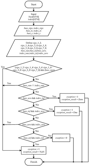
Figure 2.
Program flowchart of the preprocessing module.
The new definitions sign_1_2, sign_1_4, sign_3_4, sign_1_8, sign_3_8, sign_5_8, and sign_7_8 in Figure 2 denote that index equals 1/2, 1/4, 3/4, 1/8, 3/8, 5/8, and 7/8, respectively. Although the inputs base and index have quite a wide range around their numerical values, both of them are still rational numbers, which means that base and index can be expressed by p/q where p and q are two integers with the denominator q not equal to 0. Denote base = p1/q1 and index = p2/q2. When the denominator q2 is even, base must be nonnegative. This is difficult to check in an actual implementation, as p2 and q2 of index are difficult to confirm when index is an irregular high-precision FP number. In this paper, we only focus on eight common cases: index equals 1/2, 1/4, 3/4, 1/8, 3/8, 5/8, and 7/8. When index = 1/2, 1/4, 3/4, 1/8, 3/8, 5/8, or 7/8, and, in the meantime, base is negative (base_sign = 1), the 1-bit exception judgement signal exception of the preprocessing module is set to be 1 and the 128-bit exception output signal exception_result is set to be NaN (128′h7fff_8000_0000_0000_0000_0000 _0000_0000).
Another set of new definitions base_nan, base_inf, and base_zero (index_nan, index_inf, and index_zero) also appears in Figure 2. To be specific, base_nan (index_nan) means that the FP input number base (index) is not a number (NaN); base_inf (index_inf) means that base (index) is infinite either negatively or positively; base_zero (index_zero) means that base (index) equals to zero.
According to Figure 2, there exist certain cases the where exception judgement signal exception is set to be 1 and exception output signal exception_result is set to a corresponding numerical value. Otherwise, exception is set to be 0, which means that there is no exceptional situation in the preprocessing module. After the preprocessing module, the signals base_sign, index_sign, base_e, index_e, base_m, index_m, exception, and exception_result are transferred to next module, the QH module.
3.2. QH Module
In this paper, hardware modeling of the function XY is done through the logarithmic function lnX, the multiplication of lnX and Y, and the exponential function eYlnX. In the QH module, the implementation of the logarithmic function and the exponential function with QH CORDIC methodology in Section 2.1 is abstracted as in Figure 3.
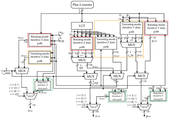
Figure 3.
Vectoring mode and rotating mode of QH CORDIC.
In Figure 3, the vectoring mode of the QH CORDIC is for the logarithmic function lnX, while the rotating mode of the QH CORDIC is for exponential function eYlnX. The vectoring mode of the QH CORDIC bears a close resemblance to the rotating mode of the QH CORDIC because they both have three major data paths and seven submodules. Their differences mainly lie in the signal that determines the rotation direction of the next iteration (signal s_ln and signal s_exp). As explained in Section 2.2, in order to ensure the ROC of QH CORDIC, when i = 5, 13, 41, 121, ···, (3i+2 − 1)/2, ··· where i starts from 0, repeated iterations are needed. Therefore, except for the iterative X/Y/Z data path that performs the iterative formulae xn+4/yn+4/zn+4, the iterative X/Y/Z data paths when i = 5, 13, 41, 121 are also listed.
The actual implementation of the QH module establishes a finite state machine (FSM), which has twelve states: INIT_LN, ITE_LN, ONE_STEP_1_LN, ONE_STEP_2_LN, INNER_DEAL_0, INNER_DEAL_1, INNER_DEAL_2, INNER_DEAL_3, INIT_EXP, ITE_EXP, ONE_STEP_1_EXP, and ONE_STEP_2_EXP.
As for the twelve states, the states INIT_LN, ITE_LN, ONE_STEP_1_LN, and ONE_STEP_2_LN belong to the logarithmic function calculating part; the states INIT_EXP, ITE_EXP, ONE_STEP_1_EXP and ONE_STEP_2_EXP belong to the exponential function calculating part; the state INNER_DEAL_0 performs the post-processing of logarithmic function; the state INNER_DEAL_1 belongs to multiplication part; the state INNER_DEAL_2 performs the multiplication in preprocessing of exponential function; the state INNER_DEAL_3 performs the additions in preprocessing of exponential function. A detailed state transition diagram of the FSM is presented in Figure 4.
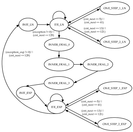
Figure 4.
State transition diagram of the finite state machine.
To some extent, the architectures of the twelve states are parallelly similar. Figure 5 shows the initialization process of the logarithmic function and the exponential function. In Figure 5a, z_in = {base_m, 35′b0} where base_m is one of the outputs of the preprocessing module. In Figure 5b, K_inv is a constant and its value is as Equation (12).
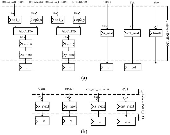
Figure 5.
(a) Architecture of the state INIT_LN; (b) architecture of the state INIT_EXP.
Input exp_pre_mantissa is one of the outputs of the state INNER_DEAL. The architecture of the states INNER_DEAL_0, INNER_DEAL_1, INNER_DEAL_2, and INNER_DEAL_3 is shown in Figure 6.
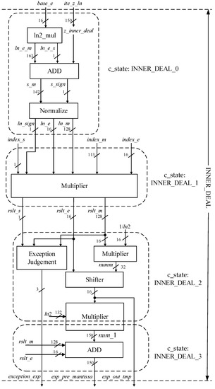
Figure 6.
Architecture of states INNER_DEAL_0, INNER_DEAL_1, INNER_DEAL_2, and INNER_DEAL_3.
In Figure 6, the external inputs are index_s, index_m, index_e, base_e, ite_z_ln, and a constant 1/ln2. Among them, index_s, index_m, index_e, and base_e are the outputs of the preprocessing module, while ite_z_ln is one of the outputs of the module z_pre in the state ITE_LN.
The state INNER_DEAL_0 in Figure 6 realizes the normalization of the calculated results base_e and ite_z_ln after the states INIT_LN, ITE_LN, ONE_STEP_1_LN, and ONE_STEP_2_LN, while the state INNER_DEAL_0 turns the results of logarithmic function lnX into a normalized 128-bit FP number {ln_sign, ln_e, ln_m}.
INNER_DEAL_1 in Figure 6 computes the multiplication of two 128-bit FP numbers, lnX and Y. The result of INNER_DEAL_1 is also a normalized 128-bit FP number {rslt_s, rslt_e, rslt_e}.
The states INNER_DEAL_2 and INNER_DEAL_3 realize predealing of the 128-bit FP input {rslt_s, rslt_e, rslt_e} of exponential function eYlnX, including exception checking and ensuring the computational validity problem of the exponential function. Generally, state INNER_DEAL_2 performs the former multiplication operation while state INNER_DEAL_3 performs the later multiplication operation and an addition operation.
Figure 7a,b demonstrate the architectures of state ITE_LN and state ITE_EXP, respectively. The yellow box in Figure 7a corresponds to the yellow box in Figure 3, while the red box in Figure 7b corresponds to the red box in Figure 3. Module x_pre in Figure 7a,b is the same, so it is with the module y_pre and the module z_pre. The three important modules x_pre, y_pre, and z_pre consist of iterative data paths of xn+4, yn+4, and zn+4 in Equation (2). Furthermore, the signal in the register cnt_next and signal exception determine the next state after ITE_LN or ITE_EXP.
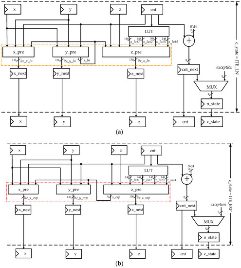
Figure 7.
(a) Architecture of the state ITE_LN; (b) architecture of the state ITE_EXP.
The architecture of module x_pre is shown in detail in Figure 8. The module x_pre is performs iterative X data path calculation and involves many multiplications with single integer constants. Binary decomposition is used to encode single integer constants to reduce delay. Module x_pre divides the iterative X data path into three layers. Layer1 evaluates 2, 4, 8, 16, and 32 times of the inputs x and y with shift operations. Layer2 uses the results of layer1 and the binary decomposed results of single integer constants with a series of compressors and adders to obtain 9, 15, 19, 21, and 35 times the input x, and 3, 5, 7, 9, 11, 13, and 15 times the input y. Layer3 performs shift and compress operations on the results of layer2 according to Equation (2).
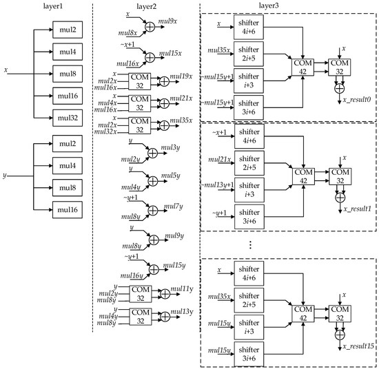
Figure 8.
Architecture of the module x_pre.
Architecture of the module y_pre is quite similar to module x_pre. Iterative Z data path calculation is also optimized and its architecture is shown in Figure 9.
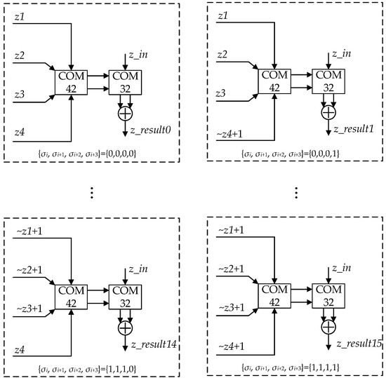
Figure 9.
Architecture of module z_pre.
The iterations of the Z data path require 16 calculations for the inputs {σn, σn+1, σn+2, σn+3} from 0000 to 1111 to obtain 16 results. The calculating process of each result is quite similar. Figure 9 takes {σn, σn+1, σn+2, σn+3} = {0, 0, 0, 0} as an example.
Figure 10a,b demonstrate architectures of the state ONE_STEP_1_LN and state ONE_STEP_2_LN, respectively. The two green boxes in Figure 10a,b jointly make up the repetitive iterative xn+4, yn+4 and zn+4 data path for logarithmic functions. However, when register cnt is 5 or 41, the FSM jumps to state ONE_STEP_1_LN; when register cnt is 13 or 121, the FSM jumps to state ONE_STEP_2_LN.
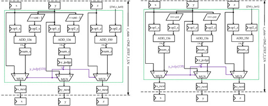
Figure 10.
(a) Architecture of the state ONE_STEP_1_LN; (b) architecture of the state ONE_STEP_2_LN.
Figure 11a,b demonstrate architectures of State ONE_STEP_1_EXP and state ONE_STEP_2_EXP, respectively. The two blue boxes in Figure 11a,b jointly make up the repetitive iterative xn+4, yn+4 and zn+4 data path for exponential functions.
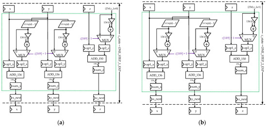
Figure 11.
(a) Architecture of the state ONE_STEP_1_EXP; (b) architecture of the state ONE_STEP_2_EXP.
3.3. Postprocessing Module
After the QH module, the outputs x_out, y_out, exp_out, and exception_out are generated. As Figure 12 shows, the signal exp_pre_exp is just exp_out of the QH module and signal exception_out_inner is exception_out of the QH module. The postprocessing module mainly serves to merge a normalized 128-bit FP output of powering function XY.
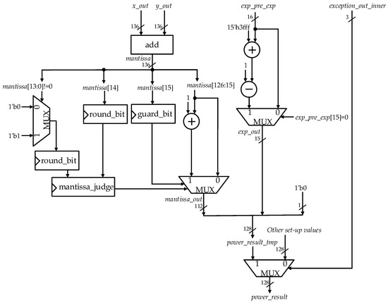
Figure 12.
Architecture of the postprocessing module.
4. Implementation Results and Comparisons
4.1. ASIC Implementation Results of the Proposed Architecture
The proposed architecture was coded in Verilog HDL and synthesized with the TSMC 65 nm standard cell library, using Synopsys Design Compiler. The proposed architecture was synthesized with the best achievable timing constraints, with the constraint of the max-area set to zero and a global operating voltage of 0.9 V. The ASIC implementation details are shown in Table 3.
Table 3.
ASIC Implementation Details @ TSMC 65 nm.
ATP and total energy are usually used to properly and roundly evaluate ASIC performance. The smaller the ATP and total energy are, the better the ASIC design. In a similar way, according to the definitions of energy efficiency and area efficiency, the smaller the energy efficiency is and the larger the area efficiency is, the better the ASIC design.
4.2. Evalutation and Comparative Analysis
In order to reveal the superiority of our approach based on the same conditions, this paper makes a comparative analysis using different indicators against other state-of-the-art approaches for computing XY-like functions, including computation correctness, word length, computation latency, and power consumption.
4.2.1. Computational Correctness
In Python, we verify the computational correctness of the proposed architecture and other approaches by evaluating their relative errors. The definition of the indicator relative error (RE) is as Equation (13):
where VT stands for the theoretical value of function XY and VM stands for the measured value of function XY with the proposed and other approaches. The maximum relative error is denoted as max(REk) of k test quantities. Another important indicator, the average relative error (ARE), is defined as Equation (14):
where k stands for test quantity of function XY.
Currently, only [12,14] in the state-of-the-art approaches implement both and XN computation. For [12,14], the test quantity k is 40,000. For [14], the number of iterations n is set to be 10. For [12], 1024 pieces of result data are stored in either LUT1 or LUT2. Software verification of [12,14] and the proposed architecture for function XY is presented in Table 4.
Table 4.
Verification of [12,14] and the proposed architecture by Python simulation.
From Table 4, in terms of max(RE) and ARE, it is evident that the proposed architecture for computation is superior compared with the state-of-the-art approaches [12,14]. The proposed architecture for XN computation is also superior compared with the state-of-the-art approaches [12,14].
4.2.2. Word Length
In this subsection, this paper analyzes the word length required for each approach’s hardware implementation based on the conditions in Section 4.2.1. The longer the word length is, the better the precision.
The word lengths of each module in [12,14], and the proposed architecture are shown in Table 5. By contrast, the word length of the proposed architecture is much longer than the state-of-the-art approaches, which means that the proposed architecture has the characteristic of high precision. However, the long word length consumes more area and power, increases the critical path, and lowers the working frequency to some extent.
Table 5.
Word length for [12,14] and the proposed architecture.
4.2.3. Timing Analysis and Power Analysis
In this section, this paper first analyzes computation latency of [14,15] and the proposed architecture to calculate or XN.
NL refers to latency savings compared with other architectures and it is defined as Equation (15):
where L is latency. Compared with [14,15], the percentage of NL is as Equation (16):
Under the circumstances, we can calculate NL, PNL for [14,15] and the proposed architecture, as shown in Table 6.
Table 6.
Timing analysis for [14,15] and the proposed architecture.
From Table 6, for computation, the proposed architecture saves 2.56% and 12.64% latency compared with [14,15], respectively. For XN computation, the proposed architecture saves 3.79% and 12.64% latency, respectively. The direct comparison of latency in terms of cycle is not fair, as the periods of [14,15] and the proposed architecture may be different. Hence, the indicator total time is employed to measure the timing efficiency of the three architectures. According to Table 6, the total time of the proposed architecture is about 6 times that of [14] and about 2.8 times that of [15]. It should be noticed that the comparison is done in terms of total time without taking into account the fact that the three architectures run on different technologies.
For fairness, the indicator throughput was also measured. From Table 6, for computation, the proposed architecture has ≈35.4% and ≈3.2% throughput overhead over [14] and [15], respectively; for XN computation, the proposed architecture has ≈37.1% and ≈3.2% throughput overhead over [14,15], respectively. It can be inferred that the throughput of our proposed architecture is larger, as our precision is much higher. For high-precision applications, the proposed architecture can achieve better timing performance.
Next, this paper focuses on the power consumption to calculate or XN for [14,15] and the proposed architecture. Similar with Section 4.1, this paper employs energy efficiency to compare with other architectures.
As seen in Table 7, the proposed design for computation saves 25.44% and 34.18% energy efficiency when it is compared with [14,15], respectively. For XN computation, our design can save 21.58% and 34.18% energy efficiency compared with [14] and [15], respectively.
Table 7.
Power analysis for [14,15] and the proposed architecture.
5. Conclusions
In this paper, a novel hardware architecture is proposed based on the QH CORDIC methodology to compute XY-like functions. The computation of function XY is divided into the computation of function lnX, a multiplication operation, and function ex, of which function lnx and function ex are calculated using the QH CORDIC.
The QH CORDIC methodology merges four single iterations into a whole parallel iteration, simultaneously computes a total of 16 possible values of xn+4, yn+4, and zn+4 respectively, and picks up rotation directions of the next iteration according to zn+4 for rotating mode or yn+4 for vectoring mode. Compared with traditional hyperbolic CORDIC algorithms, the QH CORDIC only needs 32 clock cycles to achieve 128-bit FP data accuracy, which greatly reduces the circuit latency.
The proposed architecture solves the problem of limited ROC of CORDIC algorithm and explains the validity of computing function lnx and ex with the QH CORDIC, ensuring that the domain of inputs for the proposed architecture are high-precision (128 bits) floating-point numbers.
The ASIC implementation results show that the proposed architecture’s circuit latency, area, and power consumption are 76 cycles, 1417366 μm2, and 36.2189 mW, respectively, under a working frequency of 300 MHz and a precision of at least 113 bits. The conspicuous timing performances of the proposed architecture with high-precision inputs and dramatically accurate outputs are achieved at the cost of area and power consumption. This is related to the adopted QH CORDIC methodology to a large extent, as the QH CORDIC follows the parallel computing strategy.
Compared with other architectures, the entire logic path turned out to be minor error and high accuracy. The proposed architecture is about 30 orders of magnitude superior to [12,14] in terms of max(RE) and ARE. The proposed architecture was also proved to be low-latency. For computation, the proposed architecture has 2.56% and 12.64% latency overhead over [14,15], respectively. For XN computation, it has 3.79% and 12.64% latency overhead over [14,15], respectively. In addition, the proposed architecture outmatches [14,15] in terms of indicator energy efficiency and throughput. The word length of the proposed architecture is 128 bits, three or four times that of [12,14].
Therefore, the proposed architecture is highly favored to perform high-precision floating-point computing of XY-like functions. However, the long word length may weaken the advantages in terms of area and power. Our focus in the future will firstly be rigorous error analysis that cuts down on the word length of xn+4, yn+4, and zn+4 during the QH CORDIC iterations. Secondly, the word length of the two multipliers Y and lnX can be shortened with the accuracy of product YlnX maintained. In this way, the computation of YlnX in eYlnX can be simplified. These improvements will help to reduce the total area and power of the circuit design.
In addition, the proposed hardware architecture can be modified into a low-latency and minor-error architecture for XY-like functions whose inputs are configurable in terms of precision. In line with the precisions of current scientific computing applications, not only quadruple precision (128 bits), but also half-precision (16 bits), single precision (32 bits), and double precision (64 bits) are accessible in the configurable architecture.
Author Contributions
Conceptualization, M.L.; methodology, M.L.; software, J.X. and M.L.; validation, J.X. and M.L.; writing—original draft preparation, W.F.; writing—review and editing, W.F. and M.L.; funding acquisition, M.L. All authors have read and agreed to the published version of the manuscript.
Funding
This research was funded by a project of the Educational Commission of Guangdong Province of China (2019GKQNCX122) and Scientific Research Project in School-level (SZIIT2019KJ026).
Conflicts of Interest
The authors declare no conflict of interest.
References
- Pineiro, J.-A.; Ercegovac, M.D.; Bruguera, J.D. High-radix iterative algorithm for powering computation. In Proceedings of the 16th IEEE Symposium on Computer Arithmetic, Santiago de Compostela, Spain, 15−18 June 2003; pp. 204–211. [Google Scholar]
- Harris, D. A powering unit for an Open GL lighting engine. In Proceedings of the 35th Asilomar Conference on Signals, Systems and Computers, Pacific Grove, CA, USA, 4–7 November 2001; pp. 1641–1645. [Google Scholar]
- Zuras, D.; Cowlishaw, M.; Aiken, A.; Applegate, M.; Bailey, D.; Bass, S.; Bhandarkar, D.; Bhat, M.; Bindel, D.; Boldo, S.; et al. IEEE Standard for Floating-Point Arithmetic. IEEE Std. 2008, 754, 1–70. [Google Scholar]
- Pineiro, J.-A.; Ercegovac, M.D.; Bruguera, J.D. Algorithm and architecture for logarithm, exponential, and powering computation. IEEE Trans. Comput. 2004, 53, 1085–1096. [Google Scholar] [CrossRef]
- Antelo, E.; Lang, T.; Bruguera, J.D. Very-high radix CORDIC vectoring with scalings and selection by rounding. In Proceedings of the 14th IEEE Symposium on Computer Arithmetic, Adelaide, SA, Australia, 14−16 April 1999; pp. 204–213. [Google Scholar]
- Vazquez, A.; Bruguera, J.D. Iterative algorithm and architecture for exponential, logarithm, powering, and root extraction. IEEE Trans. Comput. 2013, 62, 1721–1731. [Google Scholar] [CrossRef]
- Oberman, S.F. Floating point division and square root algorithms and implementation in the AMD-K7/sup TM/ microprocessor. In Proceedings of the 14th IEEE Symposium on Computer Arithmetic, Adelaide, SA, Australia, 14−16 April 1999; pp. 106–115. [Google Scholar]
- Pineiro, J.-A.; Bruguera, J.D. High-speed double-precision computation of reciprocal, division, square root, and inverse square root. IEEE Trans. Comput. 2002, 51, 1377–1388. [Google Scholar] [CrossRef] [Green Version]
- Langhammer, M.; Pasca, B. Single precision logarithm and exponential architectures for hard floating-point enabled FPGAs. IEEE Trans. Comput. 2017, 66, 2031–2043. [Google Scholar] [CrossRef]
- Muller, J.M. Elementary functions: Algorithms and implementation. Math. Comput. Educ. 1997, 34, 21–52. [Google Scholar]
- Schulte, M.J.; Stine, J.E. Approximating elementary functions with symmetric bipartite tables. IEEE Trans. Comput. 1999, 48, 842–847. [Google Scholar] [CrossRef]
- Chen, H.; Yang, H.; Song, W.; Lu, Z.; Fu, Y.; Li, L.; Yu, Z. Symmetric-Mapping LUT-Based Method and Architecture for Computing XY-Like Functions. IEEE Trans. Circuits Syst. I Regul. Pap. 2021, 68, 1231–1244. [Google Scholar] [CrossRef]
- Luo, Y.; Wang, Y.; Sun, H.; Zha, Y.; Wang, Z.; Pan, H. CORDIC-based architecture for computing Nth root and its implementation. IEEE Trans. Circuits Syst. I Regul. Pap. 2018, 65, 4183–4195. [Google Scholar] [CrossRef]
- Mopuri, S.; Acharyya, A. Low complexity generic VLSI architecture design methodology for Nth root and Nth power computations. IEEE Trans. Circuits Syst. I Regul. Pap. 2019, 66, 4673–4686. [Google Scholar] [CrossRef]
- Wang, Y.; Luo, Y.; Wang, Z.; Shen, Q.; Pan, H. GH CORDIC-based architecture for computing Nth root of single-precision floating-point number. IEEE Trans. Very Large Scale Integr. Syst. 2020, 28, 864–875. [Google Scholar] [CrossRef]
- Combet, M.; van Zonneveld, H.; Verbeek, L. Computation of the base two logarithm of binary numbers. IEEE Trans. Electron. Comput. 1965, EC-14, 863–867. [Google Scholar] [CrossRef]
- Hall, E.L.; Lynch, D.D.; Dwyer, S.J. Generation of products and quotients using approximate binary logarithms for digital filtering applications. IEEE Trans. Comput. 1970, C-19, 97–105. [Google Scholar] [CrossRef]
- Abed, K.H.; Siferd, R.E. CMOS VLSI implementation of a low-power logarithmic converter. IEEE Trans. Comput. 2003, 52, 1421–1433. [Google Scholar] [CrossRef]
- Abed, K.H.; Siferd, R.E. VLSI implementation of a low-power antilogarithmic converter. IEEE Trans. Comput. 2003, 52, 1221–1228. [Google Scholar] [CrossRef]
- Paul, S.; Jayakumar, N.; Khatri, S.P. A fast hardware approach for approximate, efficient logarithm and antilogarithm computations. IEEE Trans. Very Large Scale Integr. Syst. 2009, 17, 269–277. [Google Scholar] [CrossRef] [Green Version]
- De Dinechin, F.; Pasca, B. Floating-point exponential functions for DSP-enabled FPGAs. In Proceedings of the IEEE International Conference on Field-Programmable Technology, Beijing, China, 8−10 December 2010; pp. 110–117. [Google Scholar]
- Chen, D.; Han, L.; Ko, S.B. Decimal floating-point antilogarithmic converter based on selection by rounding: Algorithm and architecture. IET Comput. Digit. Technol. 2012, 6, 277–289. [Google Scholar] [CrossRef]
- Chen, D.; Han, L.; Choi, Y.; Ko, S.-B. Improved decimal floating-point logarithmic converter based on selection by rounding. IEEE Trans. Comput. 2012, 61, 607–621. [Google Scholar] [CrossRef]
- Liu, W.; Nannarelli, A. Power efficient division and square root unit. IEEE Trans. Comput. 2012, 61, 1059–1070. [Google Scholar] [CrossRef]
- Seth, A.; Gan, W.-S. Fixed-point square roots using L-b truncation. IEEE Signal Process. Mag. 2011, 28, 149–153. [Google Scholar] [CrossRef]
- Kabuo, H.; Taniguchi, T.; Miyoshi, A.; Yamashita, H.; Urano, M.; Edamatsu, H.; Kuninobu, S. Accurate rounding scheme for the Newton-Raphson method using redundant binary representation. IEEE Trans. Comput. 1994, 43, 43–51. [Google Scholar] [CrossRef]
- Mack, J.; Bellestri, S.; Llamocca, D. Floating point CORDIC-based architecture for powering computation. In Proceedings of the 2015 International Conference on ReConFigurable Computing and FPGAs (ReConFig), Riviera Maya, Mexico, 7–9 December 2015; pp. 1–6. [Google Scholar]
- Luo, Y.; Wang, Y.; Ha, Y.; Wang, Z.; Chen, S.; Pan, H. Generalized Hyperbolic CORDIC and Its Logarithmic and Exponential Computation with Arbitrary Fixed Base. IEEE Trans. Very Large Scale Integr. Syst. 2019, 27, 2156–2169. [Google Scholar] [CrossRef]
- Duprat, J.; Muller, J.M. The CORDIC algorithm: New results for fast VLSI implementation. IEEE Trans. Comput. 1993, 42, 168–178. [Google Scholar] [CrossRef] [Green Version]
- Phatak, D.S. Double step branching CORDIC: A new algorithm for fast sine and cosine generation. IEEE Trans. Comput. 1998, 47, 587–602. [Google Scholar] [CrossRef] [Green Version]
- Fu, W.; Xia, J.; Lin, X.; Liu, M.; Wang, M. Low-Latency Hardware Implementation of High-Precision Hyperbolic Functions Sinhx and Coshx Based on Improved CORDIC Algorithm. Electronics 2021, 10, 2533. [Google Scholar] [CrossRef]
- Llamocca-Obregón, D.R.; Agurto-Ríos, C.P. A fixed-point implementation of the expanded hyperbolic CORDIC algorithm. Lat. Am. Appl. Res. 2007, 37, 83–91. [Google Scholar]
- Hao, L.; Ming-Jiang, W.; Mo-Ran, C.; Ming, L. A VLSI Implementation of Double Precision Floating-Point Logarithmic Function. In Proceedings of the 2019 IEEE 4th International Conference on Signal and Image Processing (ICSIP), Wuxi, China, 19–21 July 2019; pp. 345–349. [Google Scholar]
Publisher’s Note: MDPI stays neutral with regard to jurisdictional claims in published maps and institutional affiliations. |
© 2021 by the authors. Licensee MDPI, Basel, Switzerland. This article is an open access article distributed under the terms and conditions of the Creative Commons Attribution (CC BY) license (https://creativecommons.org/licenses/by/4.0/).