Improvement of Accuracy and Precision of the LiDAR System Working in High Background Light Conditions

Abstract

Background light noise is one of the major challenges in the design of Light Detection and Ranging (LiDAR) systems. In this paper, we build a single-beam LiDAR module to investigate the effect of light intensity on the accuracy/precision and success rate of measurements in environments with strong background noises. The proposed LiDAR system includes the laser signal emitter and receiver system, the signal processing embedded platform, and the computer for remote control. In this study, two well-known time-of-flight (ToF) estimation methods, which are peak detection and cross-correlation (CC), were applied and compared. In the meanwhile, we exploited the cross-correlation technique combined with the reduced parabolic interpolation (CCP) algorithm to improve the accuracy and precision of the LiDAR system, with the analog-to-digital converter (ADC) having a limited resolution of 125 mega samples per second (Msps). The results show that the CC and CCP methods achieved a higher success rate than the peak method, which is 12.3% in the case of applying emitted pulses 10 µs/frame and 8.6% with 20 µs/frame. In addition, the CCP method has the highest accuracy/precision in the three methods reaching 7.4 cm/10 cm and has a significant improvement over the ADC’s resolution of 1.2 m. This work shows our contribution in building a LiDAR system with low cost and high performance, accuracy, and precision.

1. Introduction

Light Detection and Ranging (LiDAR) has been one of the most important sensors in the advanced driver assistance systems (ADAS) of autonomous vehicles developed in recent years [1,2,3,4,5,6]. To achieve the fully automated level of the self-driving car, the ADAS system relies on combining several sensors such as ultrasonic, radar, camera, and LiDAR. Each type of sensor has its own advantages and weaknesses. Ultrasonic works by sound waves and has the ability to detect objects in short distances, which is suitable for parking assistance. The camera can observe the surrounding environment, but its visibility is limited at night conditions and bad weather. Furthermore, the camera cannot estimate velocity and distances, also. Radars using radio waves can determine long distances and work well at night and in poor ambient conditions, but have low resolution. LiDAR utilizes near-infrared light to detect objects, measures distances, and constructs 3D point cloud maps at high speed and accuracy. However, it is also affected by environmental conditions and has high product costs, which are considered as challenges for future development researchers [4,5,7,8]. In order for the sensors to receive the quality reflected signal at long distances as well as in harsh environmental conditions, the transmitter antenna unit plays an important role in signal transmission. A survey of circularly polarized antennas to guide the selection of an appropriate antenna is presented in [9]. The designs, challenges, and applications of the metamaterial transmission-line based antennas are reviewed in [10], and an overview of the different decoupling mechanisms with a focus on metamaterial and metasurface principles applicable to SAR and MIMO antenna systems are also expressed in [11]. LiDAR works on the principle of transmitting and receiving light, so it is greatly affected by background lights from the surrounding environment, such as sunlight and electric lights. Background noise-filtering methods are mostly based on hardware development or building algorithms using signal processing software [12,13,14,15,16,17,18,19,20]. However, the quality of the LiDAR system will also be significantly reduced when it operates in the strong light environments, detects the targets with a weak reflective surface, or the target is at a long distance away.

The architecture of the LiDAR system commonly consists of three main parts: the laser beam transmitter, the reflector laser beam capture unit, and the control and data processing block [6,7], [21] (pp. 5–6). Its basic operating principle is to detect the laser pulses reflected by the target and then calculate the ToF difference between the emitting signals and the receiving signals. An optical sensor is one of the most important components integrated in LiDAR to detect reflected beams. The Single-Photon Avalanche Diode (SPAD) sensor is a suitable choice for most detectors of a LiDAR system. Because it has highly sensitive, fast avalanche photodiodes; is low-cost; and has easy integration in the CMOS circuits, SPAD is utilized to receive laser signals through the optical system [6,17,22,23,24,25,26]. The emitting and receiving signals are synchronously digitized by ADC in full waveform or time-to-digital converter (TDC) in count-time. The ADC performs analog digitization, which can capture most of the features of the signal reflected from the target in a full waveform. With the digital data obtained from the ADC, it is easy to apply the different processing methods to improve the quality of the LiDAR system. However, one factor that affects measurement accuracy is the sampling rate of the ADC. The TDC method determines the trigger time between pulses at a fixed threshold level for ToF estimation. Meanwhile, a LiDAR often works in high noise environments, and the targets have different reflectivity, so the amplitude and width of the received pulses are distorted and overlapped. With these disadvantages, using TDC for the LiDAR system has less requirements in performance, precision, and accuracy than ADC does [15,27].

The digitized dataset of the start and stop signals is executed by appropriate signal processing algorithms to estimate ToF and distance. There are five pulse detection methods to determine the ToF in recent studies, such as leading edge detection, constant fraction detection, inflection detection, center of gravity detection, and peak detection, which have been introduced and analyzed in articles [27,28], [29] (pp. 245–249). In those methods, peak detection is evaluated as the most effective one because of its fast execution time, high accuracy, and stability precision [27]. Cross-correlation estimates the time delay based on the maximum correlation of the emitted and received signals in full waveform. It is widely utilized in applications with high noise and high accuracy requirements [30,31,32,33,34,35,36,37]. An advantage of cross-correlation method compared with peak detection is that it can easily apply interpolation methods to improve the accuracy of the discrete signals. Parabolic, cosine, and gaussian interpolation algorithms were evaluated to determine whether they have low bias errors and are easy to implement. Among them, cosine has the lowest bias error, while parabolic is the simplest method that is suitable for hardware design [38,39].

This paper builds a single-beam LiDAR system with a SPAD sensor that is highly sensitive and easily integrated into CMOS circuits. To reduce the cost, the ADCs have been selected to digitize the start/stop signals limited to 125 Msps. The signal processing system is a flexible embedded kit for data processing and is easily controlled via a personal computer. The complete LiDAR system is installed and experimented with high light intensity conditions indoors and outdoors at distances ranging from 10 m to 90 m. Peak, CC, and CCP methods for estimating ToF and distance are applied to study the effect of background light noise on the success rate, execution time, and to improve the accuracy and precision of measurements in the LiDAR system.

The rest of the paper is organized as follows. The hardware system design presented in Section 2 includes an overview of the system and a detailed design of the transmitter, receiver, signal processing units, and the complete LiDAR system. The methods for determining ToF and distance are provided in Section 3. Experimental results demonstrate that the effect of noise on system performance is evaluated in Section 4. A discussion is provided in Section 5. Finally, the conclusion is shown in Section 6.

2. Design of the System Hardware

In this section, we described the design of the proposed hardware system in detail. It is specified by Section 2.1, Section 2.2, Section 2.3 and Section 2.4, which consist of overview, emitting laser pulse block, receiving block, and signal processing block. The complete prototype system is presented in Section 2.5. Finally, to ensure that the proposed system can work well under different background noise, we performed the initial experiments presented in Section 2.6.

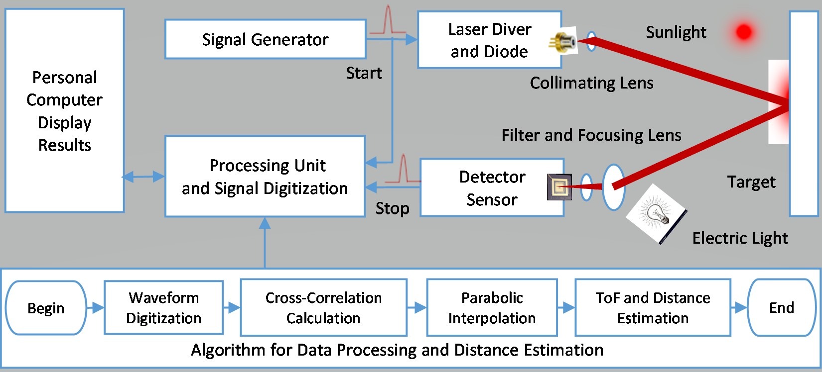
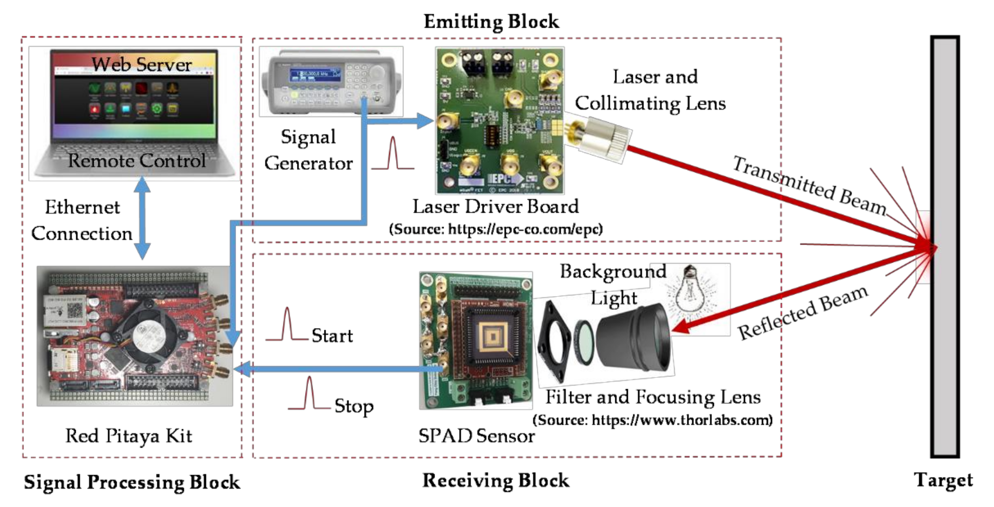
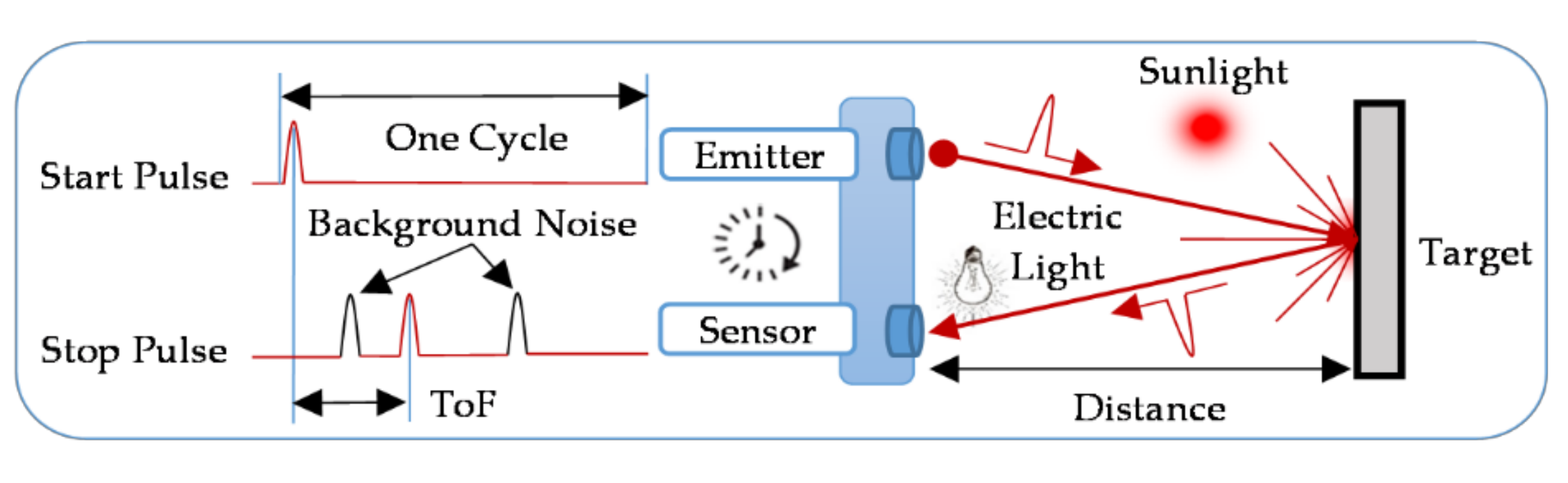
2.1. System Overview

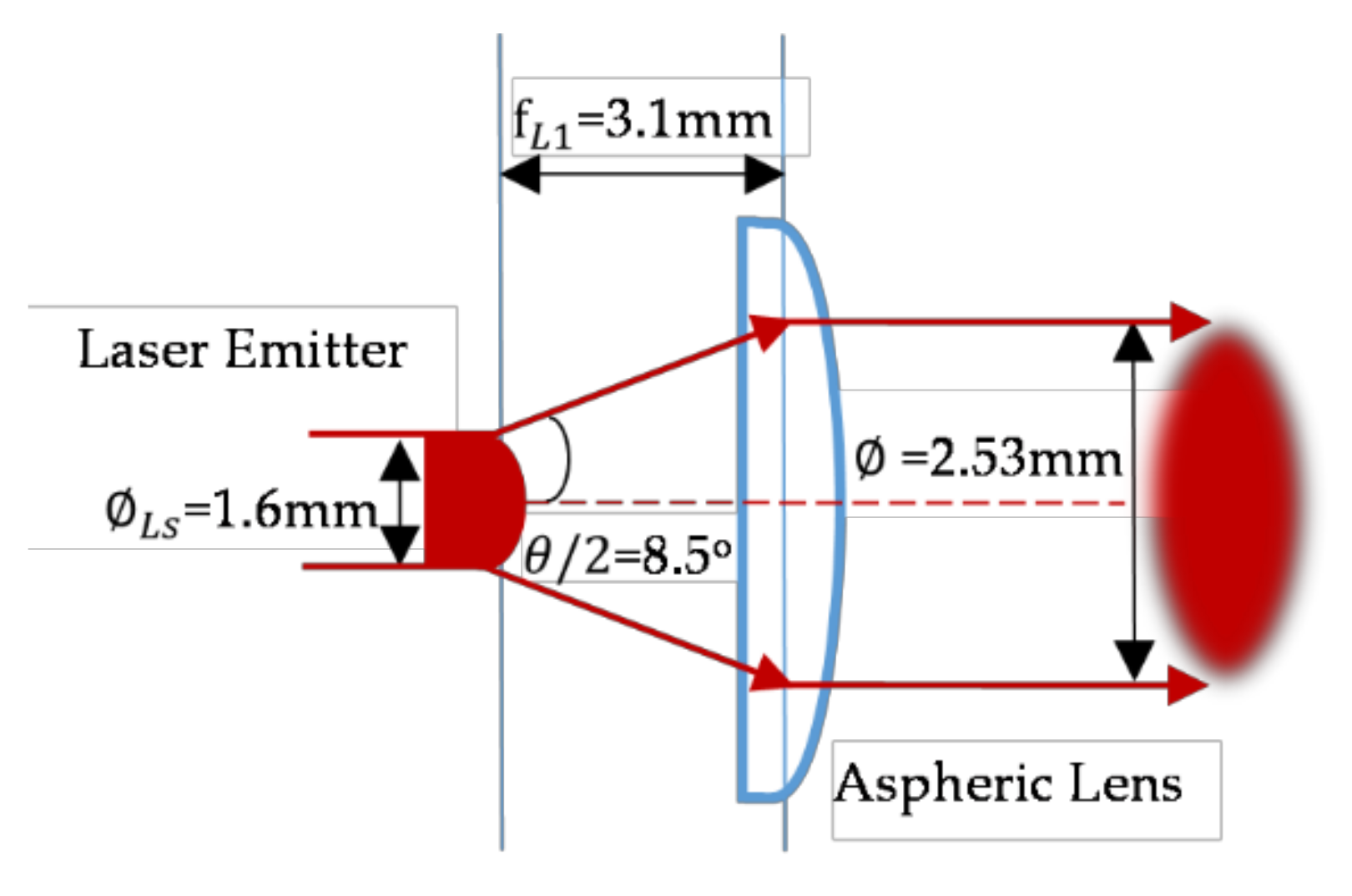
A single-beam LiDAR system consists of three blocks featuring as emitting, receiving, and signal processing units, as depicted in Figure 1. In the emitting unit, the signal generator sends a start signal in pulse form to the laser driver and the Red Pitaya concurrently; the laser driver controls the current supplied to the laser diode to emit a light beam that reaches the desired power with a high-frequency pulse source. Since the light emitted by the laser diode is a very wide beam, it should be collimated by the lens to be a narrow beam before transmitting to the target and being reflected. In the receiving unit, the focusing lens in front of the SPAD sensor collects lights reflected from the target. The received lights might consist of the expected laser signal and background noise, so a filter lens is installed near the sensor to eliminate the noise. The signal received by the sensor is also the stop signal of the measurement. In the signal processing unit, the Red Pitaya digitizes the start and stop signals and estimates the distance from the emitting position to the target. The results are shown on the personal computer and complete a measurement cycle of the LiDAR system.

2.2. Emitting Block

In this part, the narrow start pulses are generated by the function generator. Note that the pulse width of the emitting signal greatly affects the distance resolution and success rate of measurement [40]. If the starting pulses have a big width, the reflected signals will be overlapped with the original signals, and it becomes more difficult to identify stop pulses in noisy environments. Accordingly, these signals are designed with a duty cycle at a pulse width of 20 ns, which is sufficient for the ADC of the Red Pitaya board to sample at a rate of ${\mathrm{f}}_{\mathrm{s}}=125 \mathrm{Msps}$ according to the Nyquist theorem. The frequency of the selected signal is $\mathrm{f}=1 \mathrm{MHz}$ response for a common LiDAR system detecting distances from 0 to 150 m at high speed. The pulse width modulation (PWM) function of emitting signal ${\mathrm{s}}_{\mathrm{e}}\left(\mathrm{t}\right)$ is built in to Equation (1).

$${\mathrm{s}}_{\mathrm{e}}\left(\mathrm{t}\right)=\mathrm{PWM}{\left(2\mathsf{\pi }\mathrm{ft}, \mathrm{duty} \mathrm{cycle}=2\%\right)}_{ }$$

(1)

The start pulses trigger the laser diode to emit signals to the target in the form of a light beam. However, these signals are in the form of narrow pulses and high frequencies that often do not have enough power to operate the laser diode. We employed EPC9126 to address this. The EPC9126 is a laser diode driver development board that can drive laser diodes with current pulses up to 75 A and pulse width reaching 3 ns at a high repetition frequency [41]. With these capabilities of the EPC9126, it is possible to drive the laser diode to achieve the desired output power while pulse properties are maintained.

There are many types of laser sources, but laser diodes are a low cost option that can fulfill the application requirements of LiDAR [42] (p. 13). However, diode lasers typically emit an elliptical cone beam with a divergent angle, so it must be collimated by a lens to achieve a narrow beam as a point light source. Mitsubishi ML101J25 is a pulse laser diode operating at 650 nm wavelength, 250 mW peak power, and a clear aperture of ${\varnothing }_{\mathrm{Ls}}=1.6 \mathrm{mm}$ with a divergence angle of θ = 17° perpendicular to the emitter [43]. An aspherical lens with a diameter of 6.35 mm, a clear aperture of 5 mm, and a focal length of ${\mathrm{f}}_{\mathrm{L}1}=3.1 \mathrm{mm}$ is placed in front of this laser diode to collimate the laser beam as small as possible when reaching the target at long distances. The beam width after collimation calculated by Equation (2) reaches a width of $\varnothing =2.53 \mathrm{mm}$, which is small enough for a high-resolution LiDAR system. The collimating laser beam setup is shown in Figure 2.

$$\varnothing {=2\times \mathrm{f}}_{\mathrm{L}1}\times \tan \left(\raisebox{1ex}{$\mathsf{\theta }$}\!\left/ \!\raisebox{-1ex}{$2$}\right.\right)+{\varnothing }_{\mathrm{Ls}}$$

(2)

Regarding the emitting power, we know that the higher the power emitted by a laser pulse, the stronger the reflected pulse, but it must ensure safety for the human body, especially the eyes. According to the standard developed by the International Electrotechnical Commission (IEC) 60825 on equipment classification and requirements safety of laser products [44], we drive the laser diode to reach a peak power of 100 mW with an average power calculated by Equation (3) of 2 mW.

$${\mathrm{P}}_{\mathrm{avg}}{=\mathrm{P}}_{\mathrm{peak}}\times \mathrm{f}\times \Delta \mathrm{T}$$

(3)

where, ${\mathrm{P}}_{\mathrm{avg}}$ is average power; ${\mathrm{P}}_{\mathrm{peak}}$ is peak power; and $\Delta \mathrm{T}$ is pulse width.

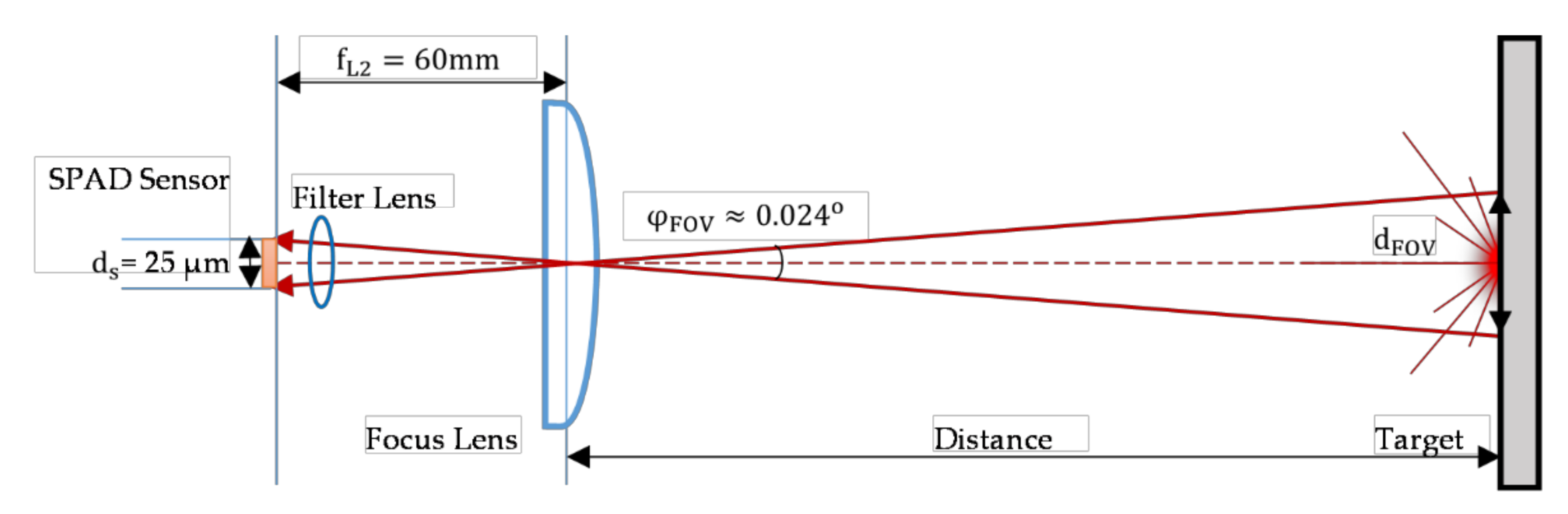
2.3. Receiving Block

In this block, a Thorlabs LA1134-A Plano-Convex focusing lens with a diameter of 25.4 mm and a focal length of ${\mathrm{f}}_{\mathrm{L}2}=60 \mathrm{mm}$ is placed in front of the SPAD sensor to capture the reflected laser beam from the target. The focal length of the lens establishes the field of view (FOV) while the diameter determines its ability to gather light. The detector sensor used in this design is the single SPAD, which has an active area of 314 µm² with an active diameter of ${\mathrm{d}}_{\mathrm{s}}=25\mathsf{\mu }\mathrm{m}$, developed by National Chiao Tung University, Taiwan [45,46,47,48,49,50,51]. As shown in Figure 3, the focusing lens can only collect reflected light from objects within the FOV. It must be calibrated so that the collected reflected beam can strongly cover the active area of the sensor. Combining the diameter of the sensor with the focal length of the focusing lens, a FOV angle determined by Equation (4) reaches ${\mathsf{\phi }}_{\mathrm{FOV}}=0{.024}^{\mathrm{o}}$. The diameters of the FOV at 10 m and 90 m distances calculated by Equation (5) achieve 4.2 mm and 37.7 mm respectively. These diameters are significantly larger than the diameter of the laser beam, demonstrating that it can capture the laser beams very well in this range.

$${\mathsf{\phi }}_{\mathrm{FOV}}=2\times \arctan \left(\raisebox{1ex}{${\mathrm{d}}_{\mathrm{s}}$}\!\left/ \!\raisebox{-1ex}{${2\mathrm{f}}_{\mathrm{L}2}$}\right.\right)$$

(4)

$${\mathrm{d}}_{\mathrm{FOV}}=2\times \mathrm{D}\times \tan \left(\raisebox{1ex}{${\mathsf{\phi }}_{\mathrm{FOV}}$}\!\left/ \!\raisebox{-1ex}{$2$}\right.\right)$$

(5)

where, ${\mathrm{d}}_{\mathrm{FOV}}$ is the diameter of FOV, D is the distance, ${\mathsf{\phi }}_{\mathrm{FOV}}$ is the angle of FOV, ${\mathrm{d}}_{\mathrm{s}}$ is the active diameter of the SPAD sensor, and ${\mathrm{f}}_{\mathrm{L}2}$ is the focal length.

LiDAR usually works in intense light environments, such as the sun or electric lights, so the signal received from the focusing lens contains a high amount of background noise. A 650 nm bandpass filter lens is installed between the laser diode and the focusing lens to eliminate light sources not in the laser’s wavelength range, as also described in Figure 3.

2.4. Signal Processing Block

Regarding the open-source embedded platform used in the signal processing block, we employed the Red Pitaya STEMLab 125-14 equipped with the dual-core ARM Cortex A9 processor working at 667 Mhz and 512 MB of RAM [52]. It also includes two fast ADCs with a sampling rate of 125 Msps and a 14-bit resolution. The waveforms of the start and stop pulses are synchronously captured by these ADCs and processed directly on the Kit. The Red Pitaya operating system is a lightweight version of Linux that a personal computer can control through the web server interface. The signal processing program is implemented in Python using Jupyter service, which is integrated into the webserver. The proposed methods for signal processing and ToF calculation are presented in Section 3.

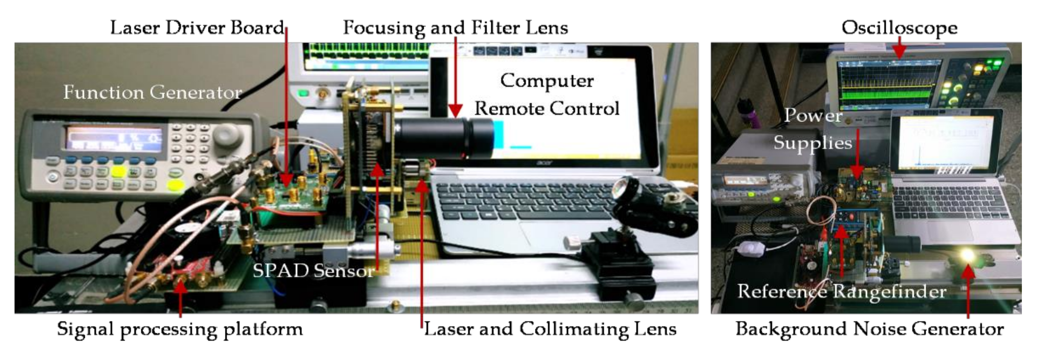
2.5. The System Prototype

The complete single-beam LiDAR experimental system is detailed in Figure 4. It consists of the laser signal transmitter and receiver system, the signal processing platform, the reference rangefinder, the background noise light generator, and the control computer. The background noise generator uses built-in ceiling electric lights, and a high-powered electric light shines directly onto the focusing lens and sensor. The rangefinder provides reference measurement values in the range of 100 m with an accuracy of ±2 mm [53].

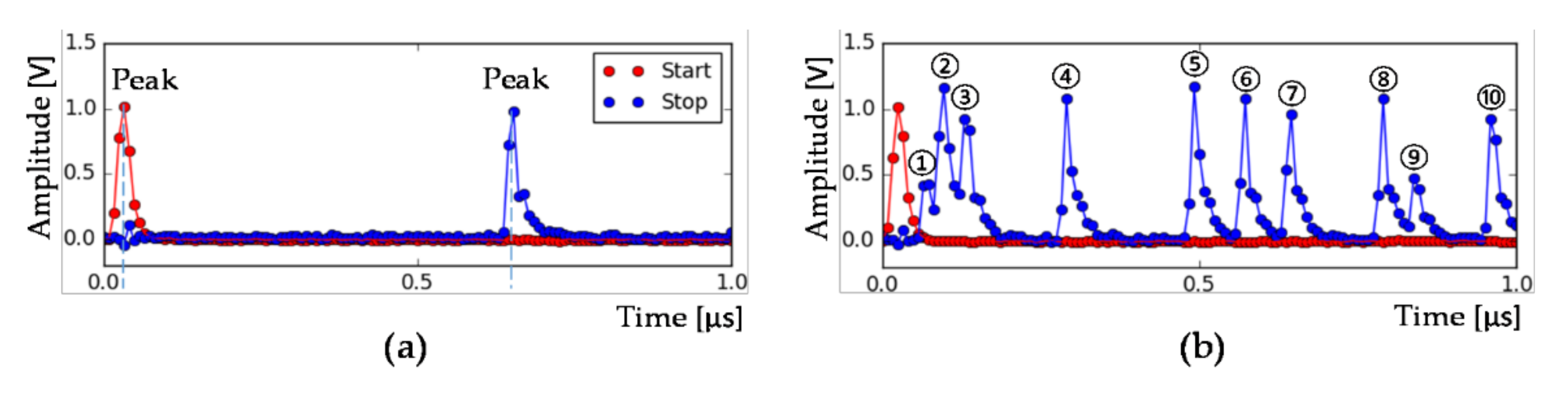
2.6. Initial Experiments

After finishing the implementation of the LiDAR system, we need to set up initial experiments to make sure if the proposed system is under the variations of background light noise. Two indoor experiments and one outdoor experiment were implemented. Indoor experiments were performed in the lab room at night in which the first experiment is with all lights off (i) and the second experiment is with ceiling lights and a background noise generator (ii). The outdoor experiment was performed under sunlight at noon (iii).

The start signals received directly from the signal generator system have an amplitude of 3 volts, and the stop pulses have an average value of approximately 1 volt. To ensure accuracy when calculating distance, we scaled the start signals by 3. The target is a white paper with 75% reflectivity.

The waveforms obtained with the target at a distance of 90 m are shown in Figure 5a–c, which correspond to experiments in cases (i), (ii), and (iii). For evaluating the ratio of the signal and the amount of background light noise in these three cases, we use a signal-to-noise ratio (SNR) indicator, which is defined by the ratio between the sum squared of the emitted signal and background noise:

$${\mathrm{SNR}=10\log }_{10}\left(\frac{{{\displaystyle \sum }}_{\mathrm{i}=0}^{\mathrm{N}}{\mathrm{V}}_{\mathrm{s}}^2\left(\mathrm{i}\right) }{{{\displaystyle \sum }}_{\mathrm{i}=0}^{\mathrm{N}}{\mathrm{V}}_{\mathrm{n}}^2\left(\mathrm{i}\right)}\right)$$

(6)

where ${\mathrm{V}}_{\mathrm{s}}\left(\mathrm{i}\right)$ is the value of the ith sample of the emitted signal, ${\mathrm{V}}_{\mathrm{n}}\left(\mathrm{i}\right)$ is the value of the ith sample of the noise, and both are measured in volts unit and have the same dimensions of N samples. The background noise signal is captured by masking the laser beam in each case correspondingly. The SNR in the three cases (i), (ii), and (iii) is determined by the Equation (6), reaching the values of 12 dB, −5.4 dB, and −9.1 dB, respectively.

The waveforms in Figure 5 shows that the received signals are smooth, indicating that the designed system works well. However, in each cycle (one start pulse), many stop pulses appear in cases of high noise (in Figure 5b,c), even though the signals are filtered by the bandpass filter lens system. This problem is because the wavelength range of the electric light and the sunlight has parts of the same wavelength as the emitted signal and occurs at many different frequencies. To accurately determine the ToF value in these instances, we apply the signal processing algorithms presented in Section 3.

3. Methodology

In this section, we introduce signal processing approaches to estimate ToF values accurately in our designed LiDAR system.

The basic principle for ToF and distance estimation of a LiDAR system is presented in Figure 6. Firstly, the start pulse is transmitted by the laser emitting system, it is then reflected by the target. After that, the sensor captures the reflected light beam that contains a transmitted signal (called a stop pulse) and background noise. ToF is the delay time between the start and stop pulse [22,23]. The measured distance is the path from the emitted pulse position to the target, calculated by the ToF value multiplied by the speed of light c and divided by two, described in Equation (7). The peak, CC, and CCP methods for estimating ToF and distance are presented in Section 3.1 and Section 3.2.

$$\mathrm{Distance}=\left(\mathrm{c} \times \mathrm{ToF}\right)/2$$

(7)

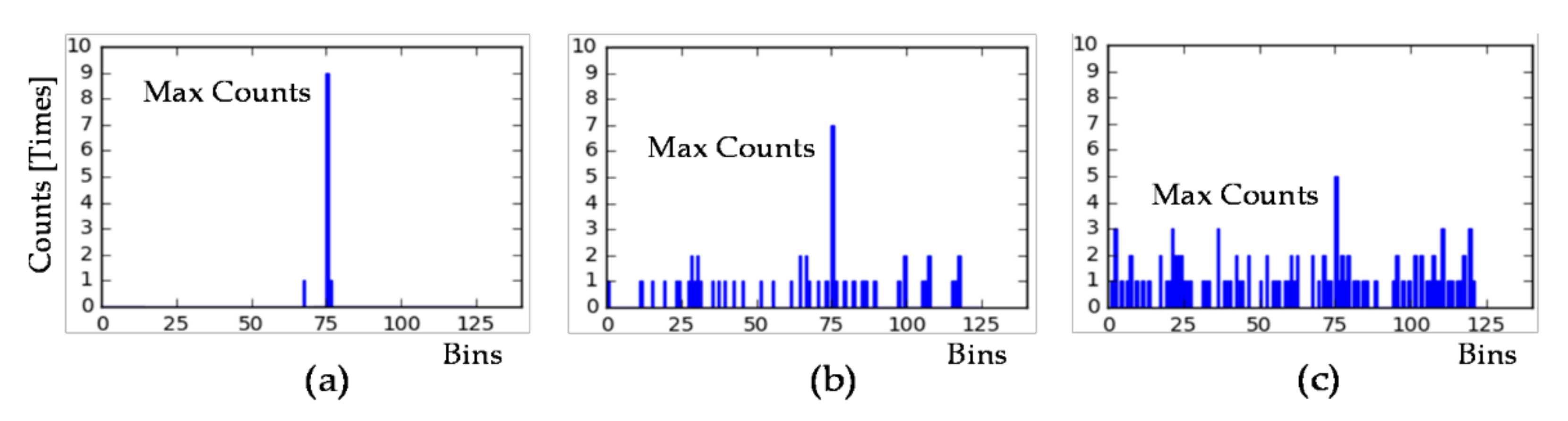
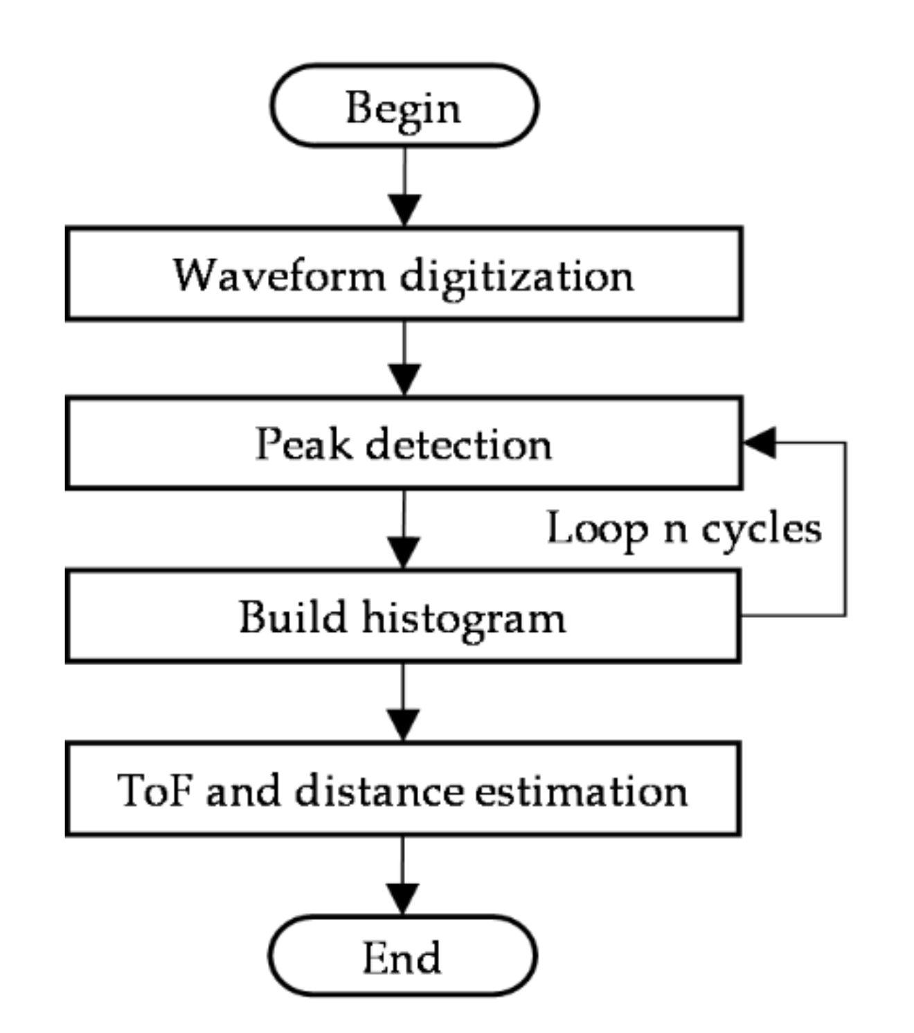
3.1. Peak Detection Method

Peak detection is a method of determining the point with the maximum amplitude value of the pulse, depicted in Figure 7a. When LiDAR operates in high noise environments, many stop pulses appear in one cycle, as shown in Figure 7b. Therefore, to accurately determine the stop pulse of the transmitted signal, the system needs to build a histogram by including the peak value of the stop pulses detected at the same time in each cycle into the histogram according to the corresponding bins [6,25,26].

Three typical histograms in Figure 8 are built in three corresponding experimental cases with increasing background noise intensity presented in Section 2.6. The histogram is constructed of 125 bins, each spaced 8 ns apart because the sampling rate of the ADC is 125 Msps (8 ns/sample), and the number of stop pulses is counted in 10 cycles. The ToF value is determined at the bin location with the largest amplitude (maximum counts), and it is converted to the distance by Equation (7).

The flowchart of the algorithm for determining ToF and distance by peak detection is shown in Figure 9. In the first step, the signal is digitized by the ADC. The second step determines the position of the stop pulses within a cycle. The third step feeds the peak value of the stop pulses to the histogram and repeats n cycles. The number of cycles is determined according to the level of background noise experienced in Section 4. The final step is to determine the ToF value and estimate the distance.

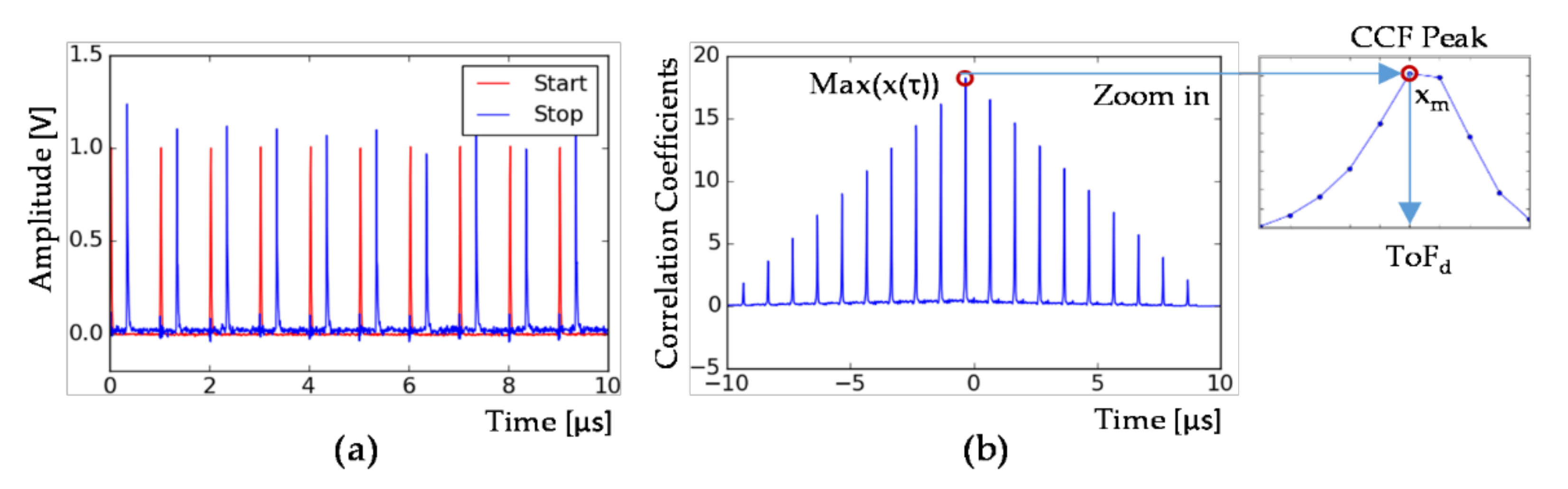
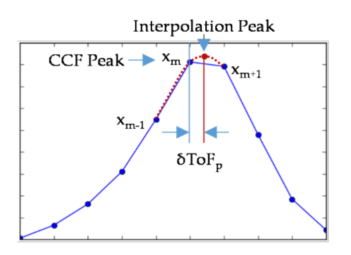
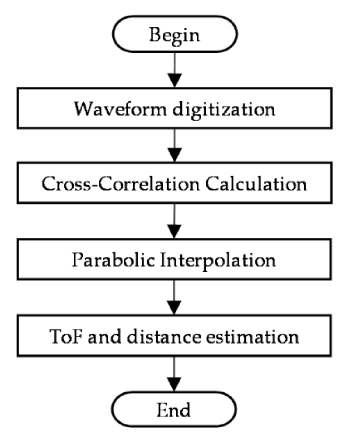
3.2. Cross-Correlation and Interpolation

The cross-correlation method determines the delay time based on the maximum correlation between the transmitted and received signals [36,38,39,54]. The received signal ${\mathrm{s}}_{\mathrm{r}}\left(\mathrm{t}\right)$ consists of the emitting signal ${\mathrm{s}}_{\mathrm{e}}\left(\mathrm{t}\right)$ delayed by a time ToF with attenuation amplitude A, and an amount of white Gaussian noise n(t):

$${\mathrm{s}}_{\mathrm{r}}\left(\mathrm{t}\right){=\mathrm{A} \times \mathrm{s}}_{\mathrm{e}}\left(\mathrm{t}-\mathrm{ToF}\right)+\mathrm{n}\left(\mathrm{t}\right)$$

(8)

The direct cross-correlation function (CCF) of two signals is determined in Equation (9), and ${\mathrm{ToF}}_{\mathrm{d}}$ is the index value at the peak point of the CCF determined in Equation (10) [39].

$$\mathrm{x}\left(\mathsf{\tau }\right)={{\displaystyle \int }}_{-\infty }^{\infty }{\mathrm{s}}_{\mathrm{r}}\left(\mathrm{t}\right){\times \mathrm{s}}_{\mathrm{e}}\left(\mathrm{t}-\mathsf{\tau }\right)\mathrm{dt}$$

(9)

$${\mathrm{ToF}}_{\mathrm{d}}=\arg [\max \left(\mathrm{x}\left(\mathsf{\tau }\right)\right)]$$

(10)

The procedure of finding ${\mathrm{ToF}}_{\mathrm{d}}$ by the direct cross-correlation method is shown in Figure 10. A start and stop signal segment in Figure 10a, after applying the CCF (9), obtained the result shown in Figure 10b. The peak of the CCF is determined at position x_m, and the ${\mathrm{ToF}}_{\mathrm{d}}$ value is determined by Equation (10).

Like the peak detection method, the cross-correlation also does not provide a better resolution than the ADC’s sampling frequency. However, it is possible to combine interpolation methods to obtain a higher resolution and accuracy. There are many interpolation techniques studied in [55,56], however, applying to a real-time system makes the system design complex, costly, and increases the execution time. Some reduced interpolation functions were introduced in [38,39]. Among them, Parabolic is a simple and effective calculation method; the error bias estimation of the time delay created by this technique is negligible. It is suitable for applying to embedded systems as well as for hardware system integration design.

The parabolic function in Equation (11) is fitted to the three maximum points of the correlation function at x_m−1, x_m, and x_m+1, as shown in Figure 11.

$${\mathrm{x}}_{\mathrm{p}}\left(\mathsf{\tau }\right){=\mathrm{c}+\mathrm{b}\mathsf{\tau }+\mathrm{a}\mathsf{\tau }}^2$$

(11)

The subsample shift estimation equation is presented by [38,39]. The peak value of the parabolic curve is the double solution of Equation (11), so we have:

$$\frac{{\mathrm{d}\mathrm{x}}_{\mathrm{p}}}{\mathrm{d}\mathsf{\tau }}=2\mathsf{\tau }\mathrm{a}+\mathrm{b}=0 \Rightarrow \mathsf{\tau }=-\frac{\mathrm{b}}{2\mathrm{a}}$$

Interpolation in intervals time 1/fs, so subsample shift is equal:

$$\mathsf{\delta }\mathrm{ToF}=\mathsf{\tau }\frac{1}{{\mathrm{f}}_{\mathrm{s}}}=-\frac{\mathrm{b}}{{2\mathrm{a}\mathrm{f}}_s}=\frac{{\mathrm{x}}_{\mathrm{m}-1} - {\mathrm{x}}_{\mathrm{m}+1}}{{2\mathrm{f}}_{\mathrm{s}}\left({\mathrm{x}}_{\mathrm{m}-1} {- 2\mathrm{x}}_{\mathrm{m}}{+\mathrm{x}}_{\mathrm{m}+1}\right)}$$

(12)

The ToF value after applying the parabolic interpolation method is the sum of the ToF_d directly calculated and the subsample shift estimation δToF_p:

$$\mathrm{ToF}={\mathrm{ToF}}_{\mathrm{d}}+{\mathsf{\delta }\mathrm{ToF}}_{\mathrm{p}}$$

(13)

The flowchart of the algorithm for determining ToF and distance by CC method combined with parabolic interpolation algorithm is described in Figure 12. In the first step, the full waveform is digitized by the ADC. The second step determines the peak value of the correlation between the start and stop signals through the CCF function. The third step applying parabolic interpolation improves measurement accuracy/precision. The final step determines the ToF value and estimates the distance.

4. Experimental Results

To research the effect of background noise on the LiDAR system, we set up the experiments under environments with different intensity lights and defined the evaluation parameters as presented in Section 4.1. Evaluation of the success measurement rate and execution time is shown in Section 4.2. The accuracy and precision are detailed in Section 4.3. Finally, the comparison of results with recent studies is mentioned in Section 4.4.

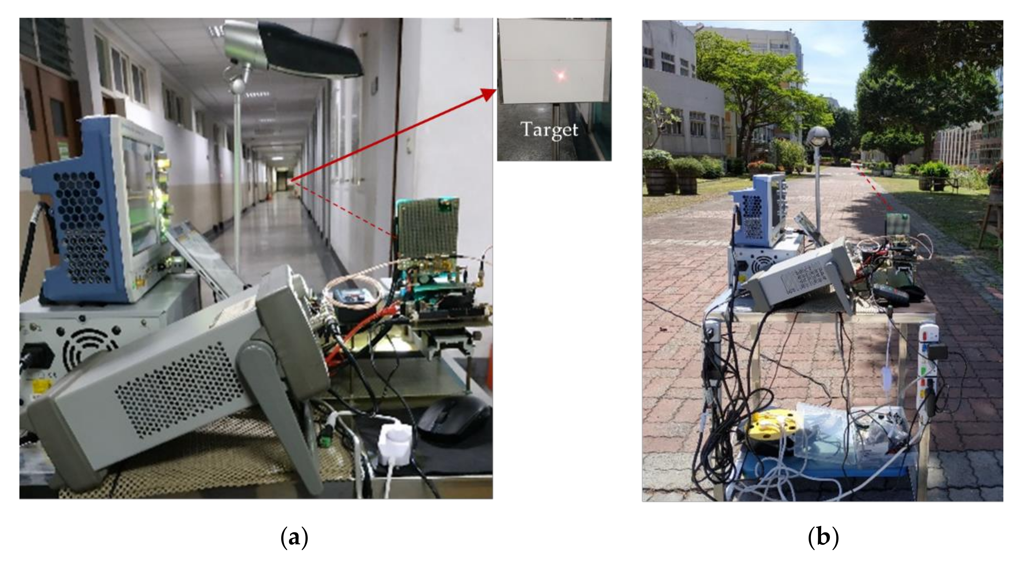
4.1. Experiment Setup and Evaluation Parameters

The experimental system in Figure 13 was setup with three different background light intensities, as introduced in Section 2.6: In Figure 13a, two experimental cases (i) and (ii) were tested in the laboratory at night with SNR 12 dB and −5.4 dB, respectively; in Figure 13b, case (iii) was performed outdoor at noon with an SNR of −9.1 dB. In each instance, we moved the target from 10 m to 90 m, with each step of 10 m. To ensure the reliability of the measurements, we performed measurement 1000 times for each distance and applied all cases.

In this study, we apply three methods to determine ToF, including peak detection, CC, and CC combined with interpolation to compare and assess the influence of background noise on the success rate, execution time, and to improve the accuracy/precision of the measurements in the LiDAR system. The measurement success rate is the percentage of correct measurements within an accepted error range over the total number of measures. With the ADC’s 125 Msps resolution (8 ns/sample), we stipulate success value of measurements within an error range of ±1 samples, which is equivalent to the accuracy of ±1.2 m (1 ns = 15 cm => 8 ns = 1.2 m). Execution time is defined as the whole performance time of signal processing algorithms for ToF estimation and distance calculation, excluding data acquisition time. The accuracy is the average value of the total error magnitude of the measurement and its actual value in the defined number of measures [27], which is determined by Equation (14). The precision represents the system’s random errors calculated from the standard deviation of the measurements in Equation (15).

$${\mathsf{\epsilon }}_{\mathrm{acu}}=\frac{1}{\mathrm{M}}{\displaystyle \sum }_{\mathrm{i}=1}^{\mathrm{M}}\left|{\mathrm{m}}_{\mathrm{i}}{-\mathrm{m}}_{\mathrm{act}}\right|$$

(14)

$${\mathsf{\epsilon }}_{\mathrm{pre}}=\sqrt{\frac{1}{\mathrm{M}}{\displaystyle \sum }_{\mathrm{i}=1}^{\mathrm{M}}{\left({\mathrm{m}}_{\mathrm{i}}{-\mathrm{m}}_{\mathrm{avg}}\right)}^2}$$

(15)

where ε_acu and ε_pre are respectively accuracy and precision of measurements, M is the total number of measurements at the same distance, m_i is the measured value at the ith times, m_act is the actual value measured from the reference rangefinder, and m_avg is the average of the measurements.

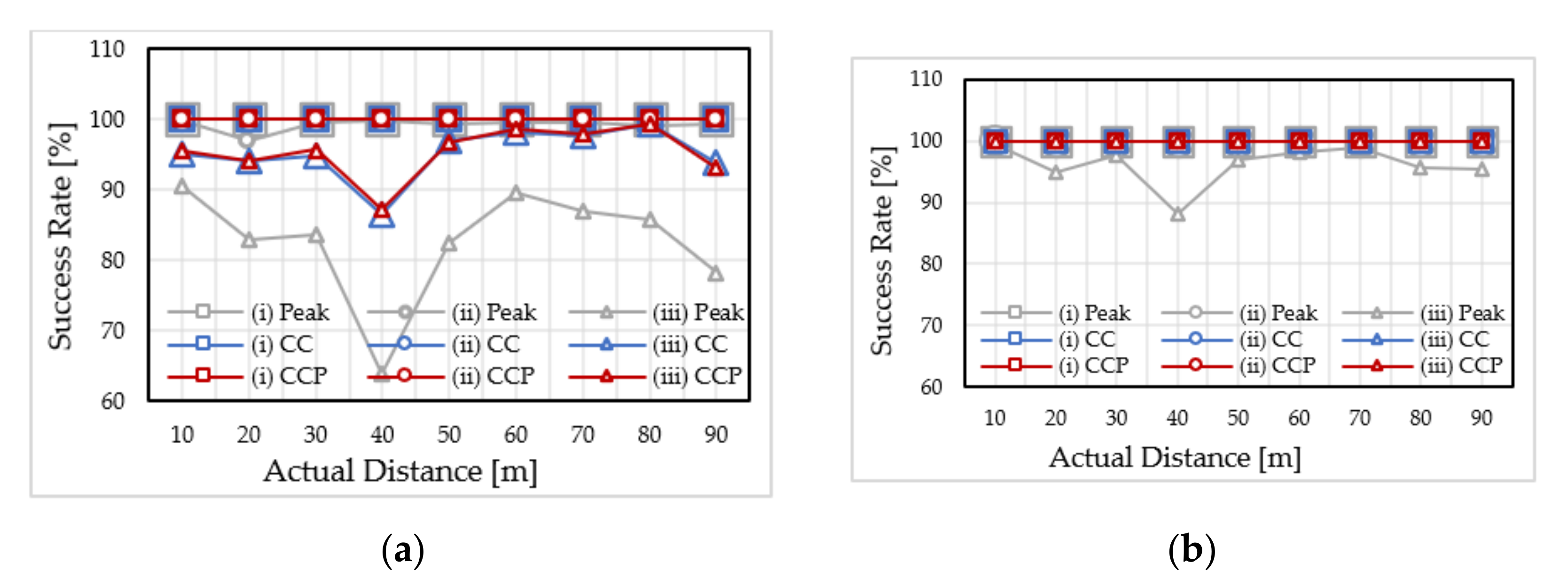
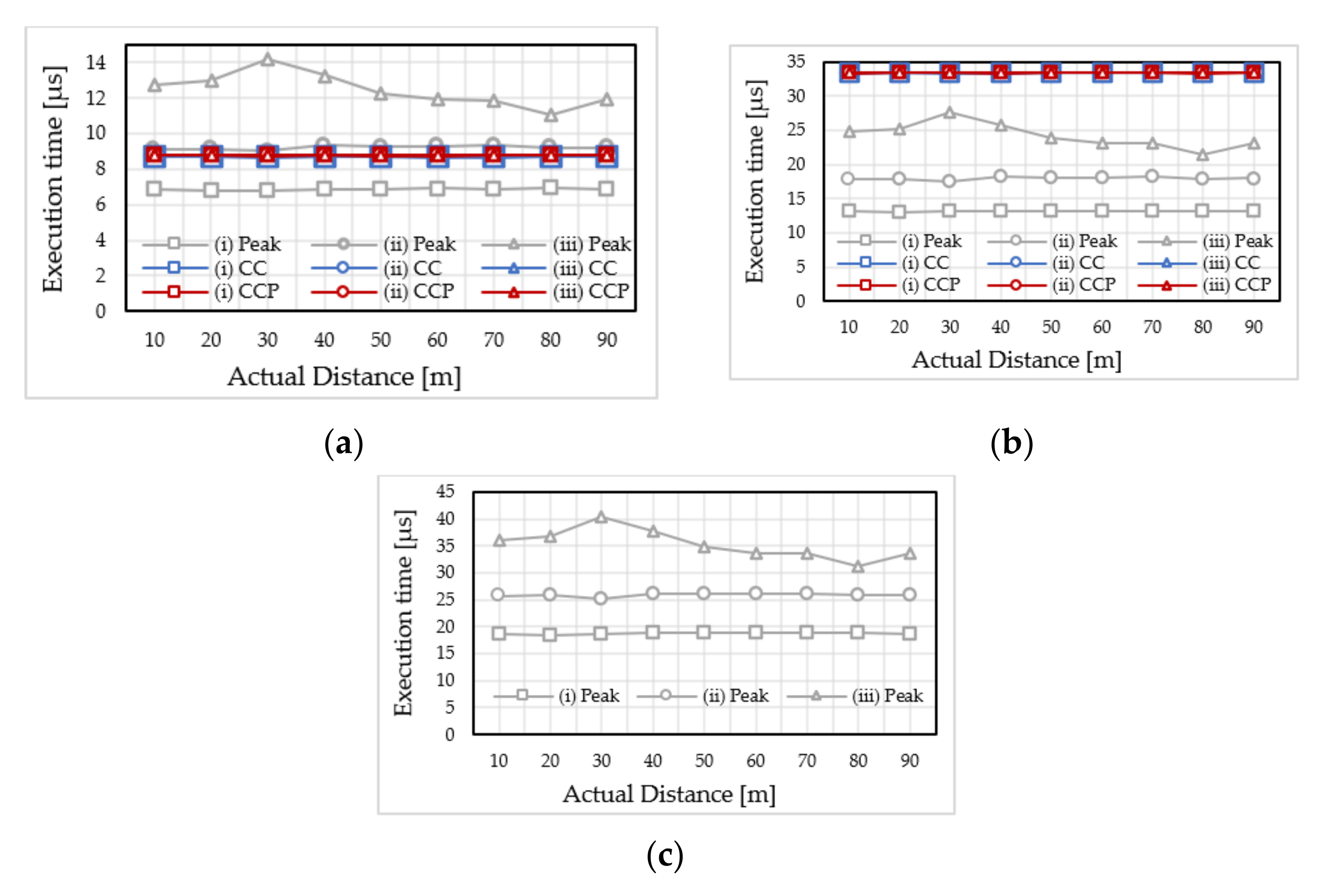
4.2. Assessing Effect of Background Light on the Success Measurement Rate and Execution Time

Under ideal conditions without noise, the system only needs to utilize one emitted pulse (one cycle) to determine the ToF value. However, in high noise environments, the system must be applied more than one start pulse per frame to identify the stop pulse accurately. In this research, we experiment in turn with 10, 20, and 30 emitted pulses per frame to evaluate the measurement’s success rate (the results in Figure 14) and execution time (the results in Figure 15) in three cases of different background light intensity ((i), (ii), and (iii)). Also, the effectiveness of the methods peak, CC, and CCP are compared.

The results of applying a frame of 10 pulses (10 μs) in the first experiment to calculate the distance are shown in Figure 14a. It shows that all three methods, peak, CC, and CCP achieve a 100% success rate in case (i) with 12 dB. In case (ii) with −5.4 dB, the CC and CCP methods reach 100%, especially the peak method achieves the lowest average rate of 99.3%. In case (iii) with −9.1 dB, there is a lower success rate. Specifically, the CC and CCP have an average rate of 95%, while the peak has the lowest average rate of only 82.7%. This result shows that the higher the background noise, the lower the success rate of the measurements. Besides that, CC and CCP methods have better performance than the peak method in high noise environments.

The second experiment in this section was performed with 20 pulses/frame (20 μs), and the results are shown in Figure 14b. In this test, only the peak method performed outdoors in case (iii) achieved an average rate of 96.1%; the rest of the instances reached 100%. This result demonstrated that the success rate would be higher when increasing the number of emitted pulses in a frame. Simultaneously, the CC and CCP also show a higher success rate than the peak method.

In another experiment, we increased the number of pulses in a frame to 30 (30 μs), and the result reached 100% in all cases, including the peak method. Through the results of three experiments, we learned that, to achieve a 100% success rate in high noise conditions, CC and CCP methods need to apply a segment of emitted pulses at least 20 μs/frame, and the peak method is 30 μs/frame.

The execution time of the first evaluation using 10 μs/frame is shown in Figure 15a. Results depicted in the chart indicate that the peak method had a longer mean execution time when the background noise varied in 12 dB, −5.4 dB and −9.1 dB. The reason is that when the noise grows, the number of stop pulses caused by noise increases, and as a result, the processing time is longer. Unlike peak detection, the average execution time of the CC method is 8.705 μs, nearly equal to that of the CCP method of 8.772 μs in all cases with different background noise. Because these two methods apply the same correlation function on all samples, their execution time is closely similar. However, the CCP method has a higher processing time than CC (0.067 μs), due to using interpolation algorithms. It also proves that the application of the interpolation method does not significantly affect the execution time of the system.

Results of the second experiment applying 20 μs/frame are shown in Figure 15b. In these results, the CC and CCP methods have the highest average execution time reach approximately 33.5 μs, the peak method performed in the case of the strongest noise is 24.2 μs. In the second experiment, the execution time of CC and CCP is higher than the peak method because the cross-correlation function convolves two arrays of the start and stop signals with doubled frame size.

In the third experiment with 30 μs/frame, we only performed with the peak method because the CC and CCP methods achieved the success rate of 100% in experiment 2. The results in Figure 15c show the average execution time of the peak method in the case of the highest background noise that reached 35.3 μs, which was larger than the CC and CCP methods in Experiment 2.

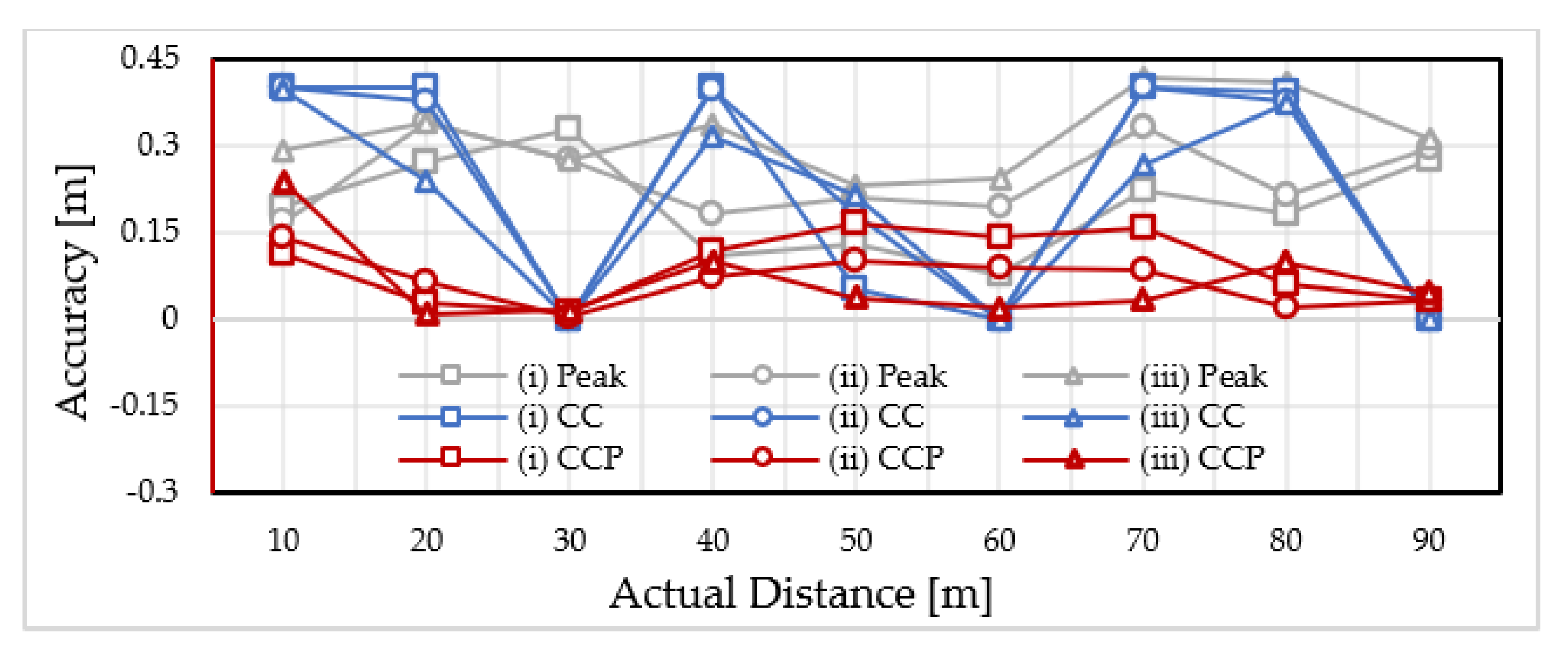
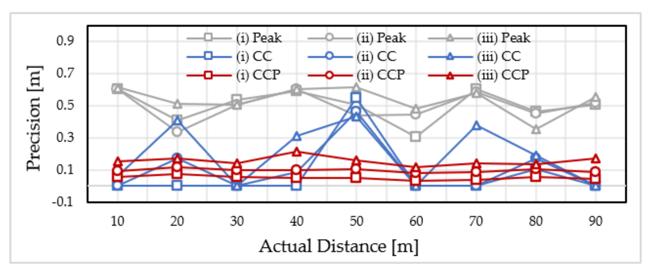
4.3. Comparing the Accuracy and Precision of Three Methods

Based on the conclusion of evaluating the success rate and execution time in Section 4.2, we only consider the instances of 30 μs/frame for the peak method and 20 μs/frame for the CC and CCP methods to compare indicators of accuracy and precision under different noisy ambient conditions.

Experimental results on the graph depicted in Figure 16 show that the peak method’s accuracy in three different cases of background noise has an average value of 0.253 m and is approximate to that of the CC method, 0.221 m. In particular, when applying the interpolation algorithm, the CCP has a very high accuracy compared to the first two methods, with an average value of 0.074 m.

Figure 17 presents the precision of peak, CC, and CCP methods under different background noise conditions (i), (ii), and (iii). The peak method has the largest error, nearly the same among experiments with an average value of 0.511 m. The CC and CCP have better precision than the peak method and have tended to decrease when background noise increases. The CC method has an average precision value of 0.122 m, whereas the CCP method is 0.1 m. These results also show that the CC method combined with the interpolation algorithm has the highest precision and stability.

4.4. Compare the Results with Recent Studies

In this section, we illustrate the effectiveness of our proposed system by comparing our results to that of the two studies [27] and [30]. In [30], the authors used the CC method to determine ToF and combined four ADCs of 500 Msps to increase the resolution of the signal. The accuracy/precision results in that study reached 30 cm (2 ns). Whereas we only used a 125 Msps ADC and applied the CC method combined with the interpolation algorithm, we can achieve better accuracy/precision values of 7.4 cm/10 cm. In addition, our proposal is low-cost and easier to implement since using multiple ADCs is costly and makes the design more complex.

In the study [27], the authors utilized an ADC with a sampling rate of 1 Gsps, eight times greater than the resolution of our experiment. This means the accuracy/precision should be eight times higher than our system. However, the results only reached an accuracy/precision of 2.43 cm/2.01 cm compared to the results in our study of 7.4 cm/10 cm. On the other hand, their experiments were performed on systems with different processing speeds, so it is difficult to compare the execution time. However, we also apply the same peak method as [27], and as a result, the CCP method has a faster execution time and better accuracy/precision than the peak method. The comparisons are detailed in

Table 1. Comparison of this work with recent studies.

Parameters	[30]	[27]	This Work
Resolution of ADC	4 × 500 Msps	1 Gsps	125 Msps
Accuracy (mean)		2.43 cm	7.4 cm
Precision (mean)	30 cm (2 ns)	2.01 cm	10 cm
Distance	7.425 m	10–46 m	10–90 m
Experiment ambient	High noise	In lab	In lab and outdoor
Processing Unit		Host Computer CPU i5-6500, 3.2 Ghz 4 GB of RAM	Embedded platform ARM Cortex A9 667 Mhz 512 MB of RAM
Number of sensors using	Two PIN sensors	Three PIN sensors	One Single-Pixel SPAD sensor

.

5. Discussion

The aforementioned results illustrated our contributions. Based on the obtained results, this discussion is about two important aspects of our proposal: the efficiency of the hardware system and the signal processing algorithms applied.

In the LiDAR system, we used a single SPAD sensor that has the advantages of high performance, low cost, easy design, and easy integration in CMOS circuits. Since the single SPAD has a small active area, when the system is designed for long-distance measurement, it has a small FOV suitable for a single-beam LiDAR system and limits the amount of background noise caused by external light sources. However, at a distance shorter than 5 m, the laser beam is almost parallel to the focusing lens, so with a small FOV, it is difficult for the system to detect the reflected signal. We can reduce the focal length to increase the FOV to measure the target at this range, but in doing so, the system cannot measure the target at the long range. Another way is to use SPADs with a larger active region to increase FOV. However, the cost will be higher, and the design will be more complicated so that choosing a suitable sensor depends on the research goal. In addition, using one or more high-resolution ADCs is costly. In this study, we only use ADC with a speed of 125 Msps combined with the CCP method, which reaches accuracy many times higher than the resolution of ADC. In most studies, an additional sensor is used to capture the start signal, which is more costly and complex in design. Instead, we take the start pulses directly from the pulse generator and scale its amplitude by an appropriate amount to ensure the correlation of the start and stop signals when calculating the distance.

The second problem to be discussed is the proposed algorithms to determine ToF and distance. The peak detection method has the advantage of fast execution under low noise conditions. However, it performs poorly in environments with high light intensity due to the appearance of many stop pulses at different frequencies. In contrast, the CC method based on the correlation of entire samples between the start and stop signals in the full waveform performs well in high noise ambience. In addition, with the CC method, applying reduced interpolation algorithms to increase accuracy and precision also does not significantly affect the execution time of the system. The results in this study orient us to design a LiDAR system with integrated SPAD sensors, ADCs, and data processing units based on CMOS technology with low-cost and high performance in the future.

6. Conclusions

This paper evaluates the influence of background light noise on the success rate and execution time of the measurements on the LiDAR system, as well as offers solutions to improve the accuracy and precision in the limited resolution of ADC. The methods for estimating ToF and distance this study include peak, CC, and CCP. Besides that, a single-beam LiDAR system is also designed with low cost and stable operation in a high noise environment to demonstrate the efficiency of these works. Experiments were carried out in the laboratory and outdoors at distances from 10 m to 90 m. The experimental results in two cases of applying emitted pulses of 10 µs/frame and 20 µs/frame showed that the CC and CCP methods had higher success rates than the peak method at 12.3% and 8.6%, respectively. Moreover, the CC method combined with a parabolic interpolation algorithm also demonstrates significantly improved accuracy/precision that reaches 7.4 cm/10 cm compared to the ADC’s resolution of 1.2 m. Our results are also compared with those of recent studies. The proposed CCP method in this study has many times higher accuracy/precision when performed under the same conditions resolution of the ADC and the ambient light noise. These results are also a reference for designing a low-cost and high-performance LiDAR system based on CMOS technology in the future.

References

1. Bengler, K.; Dietmayer, K.; Farber, B.; Maurer, M.; Stiller, C.; Winner, H. Three decades of driver assistance systems: Review and future perspectives. IEEE Intell. Transp. Syst. Mag. 2014, 6, 6–22. [Google Scholar] [CrossRef]
2. Badue, C.; Guidolini, R.; Carneiro, R.V.; Azevedo, P.; Cardoso, V.B.; Forechi, A.; Jesus, L.; Berriel, R.; Paixão, T.M.; Mutz, F.; et al. Self-driving cars: A survey. Expert Syst. Appl. 2019, 165, 113816. [Google Scholar] [CrossRef]
3. Chavez-Garcia, R.O.; Aycard, O. Multiple Sensor Fusion and Classification for Moving Object Detection and Tracking. IEEE Trans. Intell. Transp. Syst. 2016, 17, 525–534. [Google Scholar] [CrossRef] [Green Version]
4. Hecht, J. Lidar for Self-Driving Cars. Opt. Photonics News 2018, 29, 26–33. [Google Scholar] [CrossRef]
5. Zhao, M.; Mammeri, A.; Boukerche, A. Distance measurement system for smart vehicles. In Proceedings of the 2015 7th International Conference on New Technologies, Mobility and Security (NTMS), Paris, France, 27–29 July 2015; IEEE: Paris, France, 2015; pp. 1–5. [Google Scholar]
6. Rapp, J.; Tachella, J.; Altmann, Y.; McLaughlin, S.; Goyal, V.K. Advances in Single-Photon Lidar for Autonomous Vehicles: Working Principles, Challenges, and Recent Advances. IEEE Signal Process. Mag. 2020, 37, 62–71. [Google Scholar] [CrossRef]
7. Behroozpour, B.; Sandborn, P.A.M.; Wu, M.C.; Boser, B.E. Lidar System Architectures and Circuits. IEEE Commun. Mag. 2017, 55, 135–142. [Google Scholar] [CrossRef]
8. Zang, S.; Ding, M.; Smith, D.; Tyler, P.; Rakotoarivelo, T.; Kaafar, M.A. The Impact of Adverse Weather Conditions on Autonomous Vehicles: How Rain, Snow, Fog, and Hail Affect the Performance of a Self-Driving Car. IEEE Veh. Technol. Mag. 2019, 14, 103–111. [Google Scholar] [CrossRef]
9. Nadeem, I.; Alibakhshikenari, M.; Babaeian, F.; Althuwayb, A.A.; Virdee, B.S.; Azpilicueta, L.; Khan, S.; Huynen, I.; Falcone, F.; Denidni, T.A.; et al. A comprehensive survey on “circular polarized antennas” for existing and emerging wireless communication technologies. J. Phys. D Appl. Phys. 2021, 55. [Google Scholar] [CrossRef]
10. Alibakhshikenari, M.; Virdee, B.S.; Azpilicueta, L.; Naser-Moghadasi, M.; Akinsolu, M.O.; See, C.H.; Liu, B.; Abd-Alhameed, R.A.; Falcone, F.; Huynen, I.; et al. A Comprehensive Survey of “Metamaterial Transmission-Line Based Antennas: Design, Challenges, and Applications”. IEEE Access 2020, 8, 144778–144808. [Google Scholar] [CrossRef]
11. Alibakhshikenari, M.; Babaeian, F.; Virdee, B.S.; Aissa, S.; Azpilicueta, L.; See, C.H.; Althuwayb, A.A.; Huynen, I.; Abd-Alhameed, R.A.; Falcone, F.; et al. A Comprehensive Survey on “Various Decoupling Mechanisms with Focus on Metamaterial and Metasurface Principles Applicable to SAR and MIMO Antenna Systems”. IEEE Access 2020, 8, 192965–193004. [Google Scholar] [CrossRef]
12. Agishev, R.; Gross, B.; Moshary, F.; Gilerson, A.; Ahmed, S. Simple approach to predict APD/PMT lidar detector performance under sky background using dimensionless parametrization. Opt. Lasers Eng. 2006, 44, 779–796. [Google Scholar] [CrossRef]
13. Sun, W.; Hu, Y.; MacDonnell, D.G.; Weimer, C.; Baize, R.R. Technique to separate lidar signal and sunlight. Opt. Express 2016, 24, 12949–12954. [Google Scholar] [CrossRef] [PubMed]
14. Zhou, M.; Li, C.R.; Ma, L.; Guan, H.C. Land cover classification from full-waveform Lidar data based on support vector machines. ISPRS Int. Arch. Photogramm. Remote Sens. Spat. Inf. Sci. 2016, 41, 447–452. [Google Scholar] [CrossRef] [Green Version]
15. Cheng, Y.; Cao, J.; Hao, Q.; Xiao, Y.; Zhang, F.; Xia, W.; Zhang, K.; Yu, H. A novel de-noising method for improving the performance of full-waveform LiDAR using differential optical path. Remote Sens. 2017, 9, 1109. [Google Scholar] [CrossRef] [Green Version]
16. Olsen, R.C.; Metcalf, J.P. Visualization and analysis of lidar waveform data. In Laser Radar Technology and Applications XXII, Proceedings of SPIE DEFENSE + SECURITY, Anaheim, CA, USA, 9–13 April 2017; Turner, M.D., Kamerman, G.W., Eds.; SPIE: Bellingham, WA, USA, 2017; Volume 10191. [Google Scholar] [CrossRef]
17. Beer, M.; Haase, J.F.; Ruskowski, J.; Kokozinski, R. Background light rejection in SPAD-based LiDAR sensors by adaptive photon coincidence detection. Sensors 2018, 18, 4338. [Google Scholar] [CrossRef] [Green Version]
18. Zhang, X.; Wu, R.; Shen, C.; Dai, W. Anti-sunlight Jamming Technology of Laser Fuze. In Proceedings of the The 2018 International Conference on Computer Science, Electronics and Communication Engineering (CSECE 2018), Wuhan, China, 7–8 February 2018; Volume 80, pp. 59–63. [Google Scholar]
19. Mei, L.; Zhang, L.; Kong, Z.; Li, H. Noise modeling, evaluation and reduction for the atmospheric lidar technique employing an image sensor. Opt. Commun. 2018, 426, 463–470. [Google Scholar] [CrossRef]
20. Li, H.; Chang, J.; Xu, F.; Liu, Z.; Yang, Z.; Zhang, L.; Zhang, S.; Mao, R.; Dou, X.; Liu, B. Efficient lidar signal denoising algorithm using variational mode decomposition combined with a whale optimization algorithm. Remote Sens. 2019, 11, 126. [Google Scholar] [CrossRef] [Green Version]
21. McManamon, P. LiDAR Technologies and Systems; SPIE: Bellingham, WA, USA, 2019; Volume 148, ISBN 9781510625396. [Google Scholar]
22. Padmanabhan, P.; Zhang, C.; Charbon, E. Modeling and analysis of a direct time-of-flight sensor architecture for LiDAR applications. Sensors 2019, 19, 5464. [Google Scholar] [CrossRef] [PubMed] [Green Version]
23. Tontini, A.; Gasparini, L.; Perenzoni, M. Numerical model of spad-based direct time-of-flight flash lidar CMOS image sensors. Sensors 2020, 20, 5203. [Google Scholar] [CrossRef] [PubMed]
24. Niclass, C.; Soga, M.; Matsubara, H.; Kato, S.; Kagami, M. A 100-m Range 10-Frame/s 340 × 96-Pixel Time-of-Flight Depth Sensor in 0.18 μm CMOS. IEEE J. Solid-State Circuits 2013, 48, 559–572. [Google Scholar] [CrossRef]
25. Niclass, C.; Soga, M.; Matsubara, H.; Ogawa, M.; Kagami, M. A 0.18 μm CMOS SoC for a 100-m-Range 10-Frame/s 200 × 96-Pixel Time-of-Flight Depth Sensor. IEEE J. Solid-State Circuits 2014, 49, 315–330. [Google Scholar] [CrossRef]
26. Zhang, C.; Lindner, S.; Antolovic, I.M.; Mata Pavia, J.; Wolf, M.; Charbon, E. A 30-frames/s, 252 × 144 SPAD Flash LiDAR with 1728 Dual-Clock 48.8-ps TDCs, and Pixel-Wise Integrated Histogramming. IEEE J. Solid-State Circuits 2019, 54, 1137–1151. [Google Scholar] [CrossRef]
27. Li, X.; Yang, B.; Xie, X.; Li, D.; Xu, L. Influence of waveform characteristics on LiDAR ranging accuracy and precision. Sensors 2018, 18, 1156. [Google Scholar] [CrossRef] [PubMed] [Green Version]
28. Wagner, W.; Ullrich, A.; Melzer, T.; Briese, C.; Kraus, K. From Single-Pulse to Full-Waveform Scanners: Potential and Practical Challenges. Int. Arch. Photogramm. Remote Sens. Spat. Inf. Sci. 2004, 35, 201–206. [Google Scholar]
29. Shan, J.; Toth, C.K. Topograpic Laser Ranging and Scanning: Principles and Processing, 2nd ed.; CRC: Boca Raton, FL, USA; London, UK; New York, NY, USA, 2018; ISBN 9781498772273. [Google Scholar]
30. Li, C.; Chen, Q.; Gu, G.; Qian, W. Laser time-of-flight measurement based on time-delay estimation and fitting correction. Opt. Eng. 2013, 52, 076105. [Google Scholar] [CrossRef] [Green Version]
31. McCormick, M.M.; Varghese, T. An approach to unbiased subsample interpolation for motion tracking. Ultrason. Imaging 2013, 35, 76–89. [Google Scholar] [CrossRef] [PubMed] [Green Version]
32. Reddy, V.R.; Gupta, A.; Reddy, T.G.; Reddy, P.Y.; Reddy, K.R. Correlation techniques for the improvement of signal-to-noise ratio in measurements with stochastic processes. Nucl. Instruments Methods Phys. Res. Sect. A Accel. Spectrometers Detect. Assoc. Equip. 2003, 501, 559–575. [Google Scholar] [CrossRef]
33. Gan, T.H.; Hutchins, D.A. Air-coupled ultrasonic tomographic imaging of high-temperature flames. IEEE Trans. Ultrason. Ferroelectr. Freq. Control 2003, 50, 1214–1218. [Google Scholar] [CrossRef] [PubMed]
34. Lai, X.; Torp, H. Interpolation methods for time-delay estimation using cross-correlation method for blood velocity measurement. IEEE Trans. Ultrason. Ferroelectr. Freq. Control 1999, 46, 277–290. [Google Scholar] [CrossRef]
35. de Jong, P.G.M.; Arts, T.; Hoeks, A.P.G.; Reneman, R.S. Experimental evaluation of the correlation interpolation technique to measure regional tissue velocity. Ultrason. Imaging 1991, 13, 145–161. [Google Scholar] [CrossRef]
36. Parrilla, M.; Anaya, J.J.; Fritsch, C. Digital Signal Processing Techniques for High Accuracy Ultrasonic Range Measurements. IEEE Trans. Instrum. Meas. 1991, 40, 759–763. [Google Scholar] [CrossRef]
37. Nguyen, T.H.; Chabah, M.; Sintes, C. Correlation bias analysis—A novel method of sinus cardinal model for least squares estimation in cross-correlation. In OCEANS’15 MTS/IEEE Washington, Proceedings of OCEANS ’15, Washington, DC, USA, 19–22 October 2015; IEEE: Piscataway, NJ, USA, 2016; Volume 2. [Google Scholar] [CrossRef] [Green Version]
38. Céspedes, I.; Huang, Y.; Ophir, J.; Spratt, S. Methods for Estimation of Subsample Time Delays of Digitized Echo Signals. Ultrason. Imaging 1995, 17, 142–171. [Google Scholar] [CrossRef] [PubMed]
39. Svilainis, L.; Lukoseviciute, K.; Dumbrava, V.; Chaziachmetovas, A. Subsample interpolation bias error in time of flight estimation by direct correlation in digital domain. Measurement 2013, 46, 3950–3958. [Google Scholar] [CrossRef]
40. eGaN FETs for Lidar—Getting the Most Out of the EPC9126 Laser Driver. Available online: https://epc-co.com/epc/Portals/0/epc/documents/application-notes/AN027Getting-the-Most-out-of-eGaN-FETs.pdf (accessed on 25 August 2021).
41. Development Board EPC9126/EPC9126HC Quick Start Guide. Available online: https://epc-co.com/epc/Portals/0/epc/documents/guides/EPC9126xx_qsg.pdf (accessed on 21 September 2021).
42. Kaldén, P.; Sternå, E. Development of a Low-Cost Laser Range-Finder (LIDAR). Master’s Thesis, Chalmers University of Technology, Gothenburg, Sweden, 2015. [Google Scholar]
43. Laser diode Mitsubishi ML101J25. Available online: https://www.laserdiodesource.com/files/pdfs/laserdiodesource_com/8597/ML101J25_MitsubishiElectric_datasheet-1589826744.pdf (accessed on 21 September 2021).
44. Standards Australia Limited/Standards New Zealand. AS/NZS IEC 60825.1:2014; Safety of Laser Products Part 1: Equipment Classification and Requirements; Standards Australia Limited/Standards New Zealand: Sydney, NSW, Australia, 2014. [Google Scholar]
45. Hsu, F.; Wu, J.; Lin, S. Low-noise single-photon avalanche diodes in 0.25 μm high-voltage CMOS technology. Opt. Lett. 2013, 38, 55–57. [Google Scholar] [CrossRef] [PubMed]
46. Wu, J.-Y.; Lu, P.-K.; Hsiao, Y.-J.; Lin, S.-D. Radiometric temperature measurement with Si and InGaAs single-photon avalanche photodiode. Opt. Lett. 2014, 39, 5515–5518. [Google Scholar] [CrossRef]
47. Sangl, T.; Tsail, C. Time-of-Flight Estimation for Single-Photon LIDARs. In Proceedings of the 2016 13th IEEE International Conference on Solid-State and Integrated Circuit Technology (ICSICT), Hangzhou, China, 25–28 October 2016; Volume 1, pp. 750–752. [Google Scholar]
48. Huang, W.-S.; Liu, T.-H.; Wu, D.-R.; Tsai, C.-M.; Lin, S.-D. CMOS Single-Photon Avalanche Diodes for Light Detection and Ranging in Strong Background Illumination. In Proceedings of the 2017 International Conference on Solid State Devices and Materials, Sendai, Japan, 19–22 September 2017; pp. 319–320. [Google Scholar]
49. Tsai, S.Y.; Chang, Y.C.; Sang, T.H. SPAD LiDARs: Modeling and Algorithms. In Proceedings of the 2018 14th IEEE International Conference on Solid-State and Integrated Circuit Technology, ICSICT, Qingdao, China, 31 October–3 November 2018; pp. 1–4. [Google Scholar]
50. Sang, T.-H.; Tsai, S.; Yu, T. Mitigating Effects of Uniform Fog on SPAD Lidars. IEEE Sensors Lett. 2020, 4, 1–4. [Google Scholar] [CrossRef]
51. Sang, T.H.; Yang, N.K.; Liu, Y.C.; Tsai, C.M. A method for fast acquisition of photon counts for SPAD LiDAR. IEEE Sensors Lett. 2021, 5, 7–10. [Google Scholar] [CrossRef]
52. Welcome to the Red Pitaya. Available online: https://redpitaya.readthedocs.io/en/latest (accessed on 29 September 2021).
53. LD100 100M Laser Distance Meter Range Finder. Available online: https://lasertoolspecialist.com.au/product/ld100-100m-laser-distance-meter-range-finder (accessed on 30 September 2021).
54. Azaria, M.; Hertz, D. Time Delay Estimation by Generalized Cross Correlation Methods. IEEE Trans. Acoust. Speech Signal Process. 1984, 32, 280–285. [Google Scholar] [CrossRef]
55. Viola, F.; Walker, W.F. A spline-based algorithm for continuous time-delay estimation using sampled data. IEEE Trans. Ultrason. Ferroelectr. Freq. Control 2005, 52, 80–93. [Google Scholar] [CrossRef]
56. Svilainis, L. Review on Time Delay Estimate Subsample Interpolation in Frequency Domain. IEEE Trans. Ultrason. Ferroelectr. Freq. Control 2019, 66, 1691–1698. [Google Scholar] [CrossRef] [PubMed]
Figure 1. Hardware block diagram.
Electronics 11 00045 g001
Figure 2. The collimating laser beam setup.
Electronics 11 00045 g002
Figure 3. Detector field of view.
Electronics 11 00045 g003
Figure 4. The detailed installation of the LiDAR system.
Electronics 11 00045 g004
Figure 5. Waveforms are collected under different background noise environmental conditions: (a) In the lab room at night; (b) in the lab room at night with strong background light; (c) outdoor at noon.
Electronics 11 00045 g005
Figure 6. Principle of estimating ToF and distance.
Electronics 11 00045 g006
Figure 7. Signal detection by peak method in one cycle: (a) signals received at night; (b) signal with strong background light intensity appears 10 stop pulses.
Electronics 11 00045 g007
Figure 8. The histograms are built using peak detection method in 10 cycles with three cases: (a) SNR = 12 dB; (b) SNR = −5.4 dB; (c) SNR = −9.1 dB.
Electronics 11 00045 g008
Figure 9. Procedure for determining ToF and distance by peak detection method.
Electronics 11 00045 g009
Figure 10. Estimating delay time by cross-correlation method: (a) a 10 μs start and stop signal segment; (b) correlation coefficients and peak position obtained.
Electronics 11 00045 g010
Figure 11. The difference between the peak position of the CCF and the interpolation.
Electronics 11 00045 g011
Figure 12. Procedure for determining ToF and distance by CC method combined with parabolic interpolation algorithm.
Electronics 11 00045 g012
Figure 13. Photographs of the experimental setup: (a) in the laboratory at night; (b) outdoor at noon.
Electronics 11 00045 g013
Figure 14. Measurement success rate applied with the different number of transmitted pulses/frame: (a) 10 pulses/frame; (b) 20 pulses/frame.
Electronics 11 00045 g014
Figure 15. Execution time applied with the different number of transmitted pulses/frame: (a) 10 pulses/frame; (b) 20 pulses/frame; (c) 30 pulses/frame.
Electronics 11 00045 g015
Figure 16. The accuracies of the peak, CC, and CCP methods are determined in different background light environments.
Electronics 11 00045 g016
Figure 17. The precisions of the peak, CC, and CCP methods are determined in different background light environments.
Electronics 11 00045 g017