Abstract
An efficient method for the infrared and visible image fusion is presented using truncated Huber penalty function smoothing and visual saliency based threshold optimization. The method merges complementary information from multimodality source images into a more informative composite image in two-scale domain, in which the significant objects/regions are highlighted and rich feature information is preserved. Firstly, source images are decomposed into two-scale image representations, namely, the approximate and residual layers, using truncated Huber penalty function smoothing. Benefiting from the edge- and structure-preserving characteristics, the significant objects and regions in the source images are effectively extracted without halo artifacts around the edges. Secondly, a visual saliency based threshold optimization fusion rule is designed to fuse the approximate layers aiming to highlight the salient targets in infrared images and remain the high-intensity regions in visible images. The sparse representation based fusion rule is adopted to fuse the residual layers with the goal of acquiring rich detail texture information. Finally, combining the fused approximate and residual layers reconstructs the fused image with more natural visual effects. Sufficient experimental results demonstrate that the proposed method can achieve comparable or superior performances compared with several state-of-the-art fusion methods in visual results and objective assessments.
1. Introduction
Infrared (IR) and visible image fusion is a current research hot spot in image processing because of its numerous applications in computer vision tasks [1], such as military reconnaissance, biological recognition, target detecting, and tracking, etc. Infrared images can expose the thermal radiation difference of different objects, which identify the targets from the poor lighting backgrounds. IR imaging can refrain from the disturbances of such bad scenarios as low lighting, snow, rain, and fog, etc., therefore working well in the conditions of all-day/night and all-weather. However, IR images usually have low definition backgrounds and poor texture details. In contrast, visible imaging is able to capture the reflected light of an object and provide considerably high resolution and texture details; however, it is often affected by bad weather [2,3]. To obtain the plenty information for the exact understanding of a scene, most users often have to analyze the multimodality images of a scene one-by-one. However, analyzing each individual member of the multimodality images of a scene usually requires numerous resources such as more people, more time, and more money. Therefore, it is desirable to integrate multimodality images into a single image with the goal of obtaining a complementary and informative image [4,5]. The IR and visible image fusion technology attracted much attention due to its powerful ability to address the above-mentioned issues [6,7].
A large number of researches in IR and visible image fusion fields were conducted, but many existing methods suffer from some deficiencies. The traditional multiscale transform (MST) based methods can be implemented fast, but the fusion performances are poor in many conditions because of the inherent limitations of the MST-based methods [4]. For the edge-preserving filter (EPF) based fusion methods, the parameter settings of the edge-preserving filter, especially multiple parameters, are key to extract the structural details and suppress the halos artifacts [2]. If the salient feature information is not properly captured in the visual saliency (VS) based methods, it will not well highlight the vital objects/regions of source images [8]. Machine learning based methods (i.e., sparse representation and deep learning) yet are currently at an early stage and there still has great space for further investigation (e.g., the sufficient training images, fusion rule, and run time) [9,10,11].
To remedy the deficiencies mentioned above, two important concerns namely the powerful image representation/decomposition schemes and the effective image fusion rules are worthy to be insightfully explored. In this paper, a hybrid model based fusion method is proposed using the truncated Huber penalty function (THPF) smoothing based decomposition in two-scale domain, the visual saliency based threshold optimization (VSTO) fusion rule, and the sparse representation (SR) fusion rule. Extensive experiments are conducted to verify the effectiveness via comparing the proposed method with several state-of-the-art fusion approaches on the image dataset. Subjective and objective evaluations prove the superiority of our proposed method qualitatively and quantitatively.
The major contributions of this work are outlined as follows.
- •
- An effective two-scale decomposition algorithm using truncated Huber penalty function (THPF) smoothing is proposed to decompose the source images into the approximate and residual layers. The proposed THPF-based decomposition algorithm efficiently extracts the feature information (e.g., the edges, contours, etc.) and well restrains the edges and structures of the fusion results from the halo artifacts.
- •
- A visual saliency based threshold optimization (VSTO) fusion rule is proposed to merge the approximate layers. The VSTO fusion rule can suppress contrast loss and highlight the significant targets in the IR images and the high-intensity regions in the visible images. The fused images are more natural and consistent with human visual perception, which facilitate both the scene understanding of humans and the post processing of computers.
- •
- Unlike most fusion methods using sparse representation (SR) to decompose an image or merge the low frequency sub-band images, we utilize the SR based fusion rule to merge the residual layers for obtaining rich feature information (e.g., the detail, edge, and contrast). The subjective and objective evaluations demonstrate that the considerable feature information is integrated from the IR and visible images into the fused image.
The rest parts of this paper are arranged as follows. Section 2 provides the related works in the IR and visible fusion field. Section 3 details the proposed method for the IR and visible image fusion. Section 4 provides experimental setting, including the image dataset, other representative fusion methods for comparison, objective assessment metrics, and the parameter selection of the proposed THPF-VSTO-SR fusion algorithm. In Section 5, experimental results and the corresponding discussion are comprehensively presented. Finally, Section 6 gives the conclusion and discussion on future work.
2. Related Works
Various image fusion algorithms were developed in image fusion community in the past several decades [2,4,6,9,10,11,12,13,14,15]. In particular, Ma et al. [2], Jin et al. [6], Sun et al. [11], and Patel et al. [14] all gave full summaries about the IR and visible image fusion. These representative fusion methods are roughly summarized into the following categories: multiscale decomposition (MSD)-based methods, sparse representation (SR)-based methods, visual saliency (VS)-based methods, and deep learning (DL)-based methods.
MSD-based methods further comprise two types: multiscale transform (MST)-based methods and edge-preserving filter (EPF)-based methods. In the 1980s, Burt et al. [16] proposed the pyramid transform (PT)-based MST fusion approach for the first time. Since then, wavelet transform (WT) [17,18], curvelet transform (CVT) [19], contourlet transform (CT) [20], nonsubsampled contourlet transform (NSCT) [21], combination of wavelet and NSCT (CWTNSCT) [22], and nonsubsampled shearlet transform (NSST) [23] were widely used in the image fusion. The MST-based methods have achieved good performances in many applications. However, the visual artifacts (e.g., halos, pseudo Gibbs phenomenon) are commonly adverse defects for MST-based approaches [4,6]. In addition, a simple ’average’ fusion rule applied in the low frequency sub-band images often causes contrast distortions [8]. Recently, the edge-preserving filter (EPF) is introduced into the image fusion fields [2,24]. Li et al. [24] used the guided filter for image fusion aiming to get the consistency with human visual perception. Kumar [25] employed the cross bilateral filter to merge the multimodality images. Zhou et al. [26] combined the bilateral and Gaussian filters together for merging IR and visible images well. More advanced, Ma et al. [27] utilized the rolling guidance filter to decompose the source images into the base and detail layers. These representative EPF-based approaches were validated with good fusion performances due to the edge-preserving specialty.
In recent years, due to the excellent signal presentation ability of sparse representation (SR) [10], Liu et al. [28,29] adopted the sparse representation and the convolutional sparse representation (CSR) to capture the intrinsic characteristic information of source images, respectively. Meanwhile, in [30], the joint sparse representation and saliency detection (JSRSD) were used to highlight the significant objects in IR images and regions in visible images. Generally, the SR-based image fusion method consists of following steps [2,10]. (i) Input images are decomposed to overlapping patches. (ii) Each patch is vectorized as a pixel vector. (iii) Vectors are encoding as sparse representation coefficients using the trained over-complete dictionary. (iv) Sparse representation coefficients are combined via the given fusion rules. (v) The fusion result is reconstructed by the trained over-complete dictionary again. Despite SR-based methods have achieved good results in many cases, many existing methods suffer from several open-ended challenges. In [28], SR in the MST-SR based fusion method is used to merge the low-pass MST bands. However, the MST-SR-based method suffers from he information loss and block artifacts [27]. There’s also brightness loss in the CSR-based method [29]. The fusion results of JSRSD have block artifacts [30]. The above-mentioned issues cause the unnatural fusion images.
The idea of the visual saliency (VS) based method is that the important objects/regions (e.g., the outline, edge, brightness) often more easily capture people’s attentions. Bavirisetti [8] has used the mean and median filters to implement the visual saliency detection. Liu et al. [30] and Ma et al. [31] have achieved the good fusion performances with saliency analysis, respectively. The visual saliency detection is usually used to design the fusion rules.
In the last three years, the state-of-the-art deep learning (DL) was introduced into the image fusion area due to its powerful ability to process the images [9,11]. Generally, the DL-based methods can work well, because of the excellent ability of extracting the feature information from source images. Therefore, many neural network models are widely studied in image fusion fields. In [32], Li et al. have used ResNet and zero-phase component analysis, which achieve the good fusion performances. More generally, many convolutional neural networks (CNN) based methods were proposed for the IR and visible image fusion [33,34,35,36]. Unlike CNN and ResNet models, Ma et al. [37] have adopted DDcGAN (Dual-discriminator Conditional Generative Adversarial Network) to attain the fusion outputs with the enhanced targets, which facilitates the understandings of scenes for humans.
3. Methodology
The proposed THPF-VSTO-SR fusion method consists of three components: image decomposition with THPF smoothing (Section 3.1), image fusion with VSTO (Section 3.2) and SR fusion strategies (Section 3.3), and image reconstruction (Section 3.4). Figure 1 schematically illustrates the overview of image fusion method using the THPF-based decomposition and VSTO-SR fusion rule.
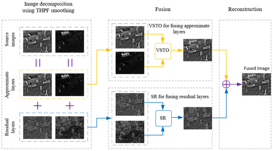
Figure 1.
Overview of image fusion method using THPF-based decomposition and VSTO-SR fusion rule (tested on ‘Road’).
3.1. Image Decomposition
The main challenges in the computer vision tasks and graphics may be attributed to the image smoothing. But in most cases, the smoothing properties for different tasks can vary considerably. It is desirable to require the smoothing operation to smooth out small details while preserving the edges and structures. In literature [38], a generalized framework for image smoothing using the truncated Huber penalty function (THPF) is presented. The smooth features of simultaneous edge- and structure-preserving can achieve better performance than that of the previous methods in many challenging situations. In this work, truncated Huber penalty function (THPF) is introduced to build a decomposition model for the first time.
3.1.1. Truncated Huber Penalty Function
The truncated Huber penalty function is defined as follows.
where a and b are constants. is the Huber penalty function [39] expressed as Equation (2).
where , which denotes a sufficient small value (typically, ).
3.1.2. Edge- and Structure-Preserving Image Smoothing Using Truncated Huber Penalty Function
Image smoothing model using truncated Huber penalty function (THPF) is defined as follows.
where f denotes an input image, and g is a guide image. The filtered output image u is the solution providing the minimum value of the above objective function Equation (3). is the same as in Equation (1); is the square patch centered at pixel i (here, = 1); is the square patch centered at i excluding pixel i (here, = 1); is a parameter controlling the whole filtering strength.
The first term of Equation (3) denotes the data term, and the second term of Equation (3) is the smoothness term in this smoothing model. (, ) and (, ) are employed to describe parameters a and b in in the data item and the smoothing item, respectively. Typically, , and , which are suggested by [38]. is the Gaussian spatial kernel given by:
where in the first term of Equation (3), and in the second term of Equation (3).
is the guidance weight defined as follows.
where the sensitivity edges in guide image g (here, ) is determined by , and is a small constant (avoiding 0 in the denominator) that is generally set as .
The numerical solution of the image smoothing model in Equation (3) is provided in the original paper.
THPF (truncated Huber penalty function)-based smoothing model can achieve simultaneous edge-preserving and structure-preserving smoothing that are rarely obtained by previous methods, which enables our fusion method to achieve better performance in the source image decomposition. In the following Section 3.1.3, we will present the detailed image decomposition based on the THPF smoothing.
3.1.3. THPF Smoothing-Based Two-Scale Image Decomposition
Due to the key edge- and structure-preserving characteristics of THPF smoothing, the filtered image is similar to the original image in terms of the overall appearance, thereby being conducive to maintaining feature information of original images in the fusion process. Assuming that and represent the registered infrared (IR) and visible images respectively, decomposition using THPF smoothing algorithm includes the following two steps. Mathematically, the procedure is depicted as follows.
Firstly, infrared image and visible image are filtered with THPF smoothing.
where the filtered images and denote the approximate layers of IR and visible images, respectively. indicates the filtering operation using THPF smoothing. Parameter controls the overall smoothing strength, and determines sensitivity edges of an image. The parameter settings of and will be detailed in Section 4.4.
The approximate layers of IR and visible images are shown in Figure 2(a2,b2), respectively.
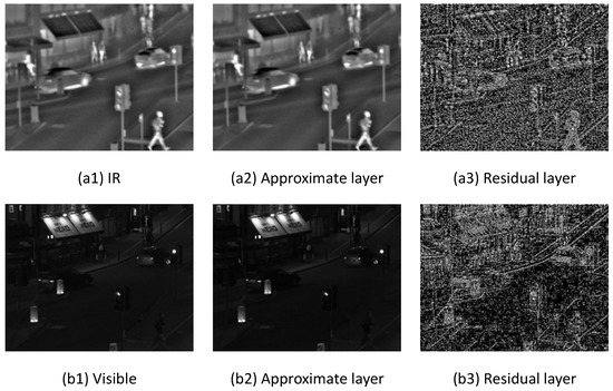
Figure 2.
Decomposition of source images using THPF smoothing (tested on ‘Road’). (a1) Infrared (IR) source image, (a2) Approximate layer of IR, (a3) Residual layer of IR, (b1) Visible source image, (b2) Approximate layer of Visible, (b3) Residual layer of Visible.
Secondly, the residual layer images and can be acquired as follows, respectively.
The residual layers of IR and visible images are shown in Figure 2(a3,b3), respectively.
3.2. Approximate Layer Fusion Using Visual Saliency-Based Threshold Optimization
The approximate layer images and contain low frequency energy information, which exhibits the overall appearance. The frequently-used and simple average fusion scheme hardly highlights the pivotal objects in infrared images and high-intensity regions in visible images, thereby often suffering from contrast distortions. Meanwhile, some fusion rules excessively pursuing salient objects either leads to over-enhancement of objects, or brings about blurred details. These phenomenons will be intuitively provided in qualitative analysis (Section 5.1). To address the above issues, it is desirable to design an efficient and appropriate algorithm for merging low frequency sub-band images. The composite images with good visual effects should be consistent with human visual perception and capture humans attentions. In view of this, a new fusion scheme using visual saliency based threshold optimization (VSTO) is proposed to merge the approximate layer images. The motivation is that human attentions are usually grabbed by objects/pixels that are more significant than their neighbors.
Morphological operations using the maximum filter are completed on the approximate layer images and for objects/regions enhancement, respectively.
where is the maximum filtering. = 3 denotes the filtering window with the window size (2r + 1)(2r + 1), typically r = 1. and are filtered images serving as the visual saliency maps (VSM) of and , respectively. Figure 3 illustrates the visual saliency maps of approximate layers for IR and visible images, as shown in Figure 3(a2,b2), respectively. Obviously, objects/regions in Figure 3(a2,b2) are easier for identification than the ones in Figure 3(a1,b1) (see comparisons in red and green boxes), respectively.
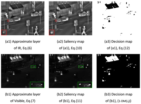
Figure 3.
Saliency and decision maps of approximate layers on source images (tested on ‘Road’). (a1) Approximate layer of IR, (a2) Saliency map of IR approximate layer, (a3) Decision map of IR approximate layer, (b1) Approximate layer of visible image, (b2) Saliency map of visible approximate layer, (b3) Decision map of visible approximate layer.
Then, decision maps of approximate layers are calculated.
where is the decision map, and denotes the initial decision matrix with binary elements ’0’ or ’1’. is the weighted matrix with the window size , here . A threshold , , is key to determining the criterion for merging more information from IR or visible approximate layer. Figure 3(a3,b3) present the decision maps of IR and visible approximate layer images, respectively.
Then, the fused approximate layer image can be acquired as follows.
From Equations (12) and (13), we can find that: As gradually increases, the fused output will merge more salient information from the visible image. Considering an extreme case of , the fused approximate layer image is the visible approximate layer image. Therefore, it is worth optimizing with the purpose of achieving the best fusion performance. Theoretically, goes from 4 to 6 (intermediate range values), thereby taking salient objects/regions in both IR and visible images into account. The fusion performance influences of will be given in Section 4.4 (iii). The proposed fusion scheme adopting visual saliency-based threshold optimization is referred to simply as VSTO.
3.3. Residual Layer Fusion Using Sparse Representation
Sparse representation (SR) and its variants are popular machine learning methods in recent years [10,40]. The core idea of sparse representation is that a signal can be represented as a linear combination of the over-complete dictionary and sparse matrix [41]. The benefit of SR is that it is more effective at finding the implicit structures and patterns from images. In many existing fusion methods, sparse representation is often used for representing/decomposing images or fusing the low frequency sub-band images. Unlike two above-mentioned ideas, SR is used to design the fusion rule for residual layer images (high frequency sub-band images) in this work. The motivation is that residual layers rather than low frequency sub-band images contain considerable structural and textural details. Thus, using SR to merge the residual layer images is very interesting and worthy of exploration.
3.3.1. Sparse Representation
For a signal ), it can be expressed as . D (, and ) denotes the over-complete dictionary. () is the sparse coefficient vector. Mathematically, can be obtained by solving the following optimization problem.
where denotes norm, and is the number of nonzero units in the sparse coefficient vector .
Then, orthogonal matching pursuit (OMP) [42], as a common greedy algorithm, is used to solve the sparse representation model with norm (Equation (14)). The K-SVD [43] algorithm is employed to train the sample signals to obtain the over-complete dictionary D. Finally, the sparse solution can be obtained.
In what follows, merging residual layers based on SR is described in detail.
3.3.2. Residual Layer Fusion
In contrast to the approximate layer images, the residual layer images and mainly contain the detail texture information. Fusing residual layer images consists of following steps.
Step 1: The residual layer images and are divided into k patches and (), respectively.
Step 2: For each patch, (or ) is converted to column vector (or ), respectively.
Step 3: In term of the pertrained dictionary D, the optimal sparse vector (or ) is solved using OMP algorithm.
Step 4: Maximum norm is selected as the evaluation criterion to obtain the fused sparse vector for the residual layer images.
where denotes norm.
Then, the fused column vector of residual layer images is calculated via the dictionary D.
Step 5: Reverse operation is performed on each vector to form the composite image, thereby achieving the fused residual layer image .
The process of residual layer fusion using sparse representation is schematically illustrated in Figure 4.
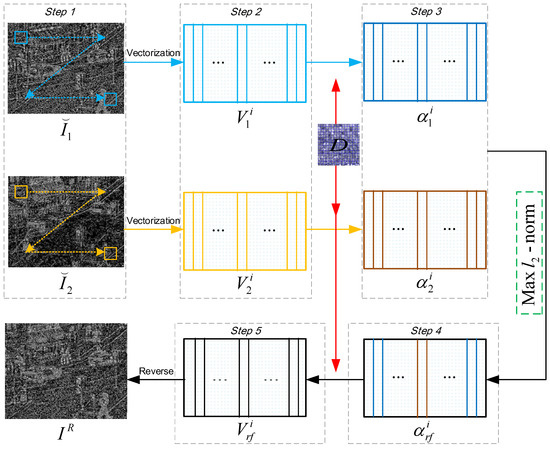
Figure 4.
Residual layer fusion using sparse representation.
3.4. Reconstruction
Finally, the fused result is reconstructed through the fused approximate layer image (Equation (13)) and the fused residual layer image (Equation (19)).
The pseudo code of the proposed algorithm is given by Algorithm 1.
| Algorithm 1 Pseudo code of proposed fusion method. |
|
4. Experimental Setting
This section presents the experimental image dataset for conducting experiments in Section 4.1, nine excellent fusion approaches for making comparisons in Section 4.2, objective assessment metrics for evaluating the fusion performance in Section 4.3, and the parameter setting of the proposed THPF-VSTO-SR fusion method in Section 4.4, respectively.
4.1. Image Data Set and Setting
Twenty preregistered IR and visible image pairs are selected to establish the experimental data set. All source image pairs are collected from the websites https://figshare.com/articles/TNO_Image_Fusion_Dataset/1008029 (accessed on 18 January 2021), and https://sites.google.com/view/durgaprasadbavirisetti/datasets (accessed on 25 June 2019), and often adopted in fusion methods. These image pairs are marked as ‘S1–S20’ respectively, as shown in Figure 5. Throughout this paper, it is assumed that all source image pairs are perfectly registered in advance. All fusion results of S1–S20 will be presented one by one in Section 5.1.
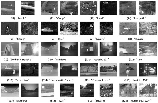
Figure 5.
Image dataset of IR and visible images. (S1–S20): ‘Bench’, ‘Camp’, ‘Road ’, ‘Sandpath’, ‘Garden’, ‘Tank’, ‘Square’, ‘Bunker’, ‘Soldier in trench 1’, ‘Movie01’, ‘Kaptein1123’, ‘Lake’, ‘Pedestrian’, ‘Houses with 3 men’, ‘Pancake house’, ‘Kaptein1154’, ‘Marne 03’, ‘Wall’, ‘Square3’, and ‘Man in door way’.
4.2. Other Fusion Methods for Comparison
To verify the effectiveness of the proposed fusion method, we conduct extensive experiments to compare our method with nine representative fusion methods, including: DWT (discrete wavelet transform) [17], CSR (convolutional sparse representation) [29], TSVSM (two-scale image fusion using visual saliency map) [8], JSRSD (saliency detection in joint sparse representation domain) [30], VSMWLS (visual saliency map and weighted least square optimization) [27], ResNet (deep learning framework based on ResNet) [32], IFCNN (image fusion framework based on convolutional neural network) [36], TE (target-enhanced) [44], and DDcGAN (dual-discriminator conditional generative adversarial network) [37].
Among these methods, DWT is multiscale transform based method. CSR and JSRSD are sparse domain based methods. TSVSM is the edge-preserving decomposition with visual salience detection method. VSMWLS is a hybrid fusion method based on edge-preserving decomposition, visual saliency map, and weighted least square optimization. TE employs a target-enhanced multiscale transform (MST) decomposition algorithm. ResNet, IFCNN, and DDcGAN are recent schemes using various state-of-the-art deep learning models, respectively. JSRSD, TSVSM, VSMWLS, and TE also are hybrid fusion methods combining the strengths of multiscale decomposition (or sparse representation) and special fusion rules (i.e., saliency detection, visual saliency map, weighted least square optimization, and target-enhanced). Generally, the first one approach is an often-used and representative multiscale transform method, while the latter eight schemes are excellent methods proposed in recent years.
For the sake of fairness, all the experimental results in this work are implemented on a desktop computer with 16 GB memory, 2.6 GHz Intel Xeon CPU, and NVIDIA GTX 1060 GPU. DWT, CSR, TSVSM, JSRSD, VSMWLS, ResNet, TE, and our method are conducted on the MATLAB 2018a environment. DDcGAN is implemented with Tensor-flow-CPU. IFCNN is carried out with PyTorch-GPU. The experimental parameters of DWT are set according to [28]. The experimental parameters of CSR [29], TSVSM [8], JSRSD [30], VSMWLS [27], ResNet [32], IFCNN [36], TE [44], and DDcGAN [37] are adopted as the same with the original papers, respectively. All the nine representative methods are conducted using the openly available codes. = 0.01, = 0.5, and are set for the proposed fusion method, and the parameter setting will be explained in Section 4.4.
4.3. Objective Assessment Metrics
Six commonly-used objective evaluation metrics are adopted to assessment the performances of various fusion methods. There are SD (standard deviation) [6], MI (mutual information) [45], FMI (feature mutual information) [46], Q (edge based on similarity measure) [47], NCIE (nonlinear correlation information entropy) [48,49], and NCC (nonlinear correlation coefficient) [2,50]. SD is the most commonly-used index reflecting the brightness differences and contrast of the fused image. MI quantifies the amount of information fused from source images to the fused image. FMI is based on MI and feature information (such as edges, details, and contrast), thereby reflecting the amount of feature information fused from source images to the fused image. Q is a very important and frequently-used metric to measure the edge information transferred from source images to the fused image. NCIE can be used to measure the general relationship between the fused image and the source images with a number from the closed interval [0, 1]. The bigger the NCIE, the stronger relationship the fused image and the source images, which indicates a good fusion performance. NCC measures how much information is extracted from the two source images. The larger the NCC, the more similar the fused image is to the source images and the better the fusion performance.
For all above metrics, large values indicate that fusion methods achieve good performances.
4.4. Parameter Analysis and Setting
For our THPF-VSTO-SR fusion method, THPF smoothing is used as the two-scale decomposition tool to extract the approximate and residual layer images. The edge- and structure-preserving characteristics of THPF smoothing based decomposition are influenced by and in Equation (6). If and vary, the performances of fusion results also change. So it is necessary to analyze the performance of our method according to parameters and . Besides, the threshold selection of in the VSTO (visual saliency-based threshold optimization) fusion rule is key to the fusion performance. These are done with help of objective evaluation metrics performing on the testing dataset consisting of 8 source image pairs (‘Bench’ (S1), ‘Camp’(S2), ‘Road’ (S3), ‘Tank’ (S6), ‘Square’ (S7), ‘Bunker’ (S8), ‘Kaptein1123’ (S11), and ‘Pedestrian’ (S13)).
(i) Fusion performance influence of : is a parameter controlling the whole filtering strength of an image. When we test the influence of the parameter on the objective evaluation metrics, and are set to 0.5 and 4, respectively.
As shown in Figure 6, the value selections of influence the average values of evaluation metrics SD, MI, FMI, Q, NCIE, and NCC on the testing dataset. Meanwhile, the value of is in the range [0.001, 1]. The metric SD remains uptrend with the value of increasing. Whereas, MI, FMI, Q, NCIE, and NCC generally keep downtrend with the value of increasing, and all achieve the peak values at = 0.01, respectively. As can be considered, = 0.01 is an eclectic but good choice.
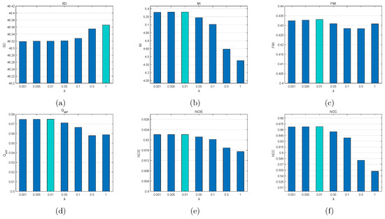
Figure 6.
Influence of parameter on objective metrics. Average values of each metric are obtained via the testing dataset. From left to right for each metric, = 0.001, 0.005, 0.01, 0.05, 0.1, 0.5, and 1. (a) SD, (b) MI, (c) FMI, (d) Q, (e) NCIE, (f) NCC.
(ii) Fusion performance influence of : determines the edge-preserving of the filtered image. Similarly, when we test the influence of the parameter on the objective evaluation metrics, and are set to 0.01 and 4, respectively.
Figure 7 presents the influence of the parameter . Obviously, SD remains uptrend with the value of increasing and achieves the highest value when = 1. However, other metrics MI, FMI, Q NCIE, and NCC keep downtrend with the value of increasing, and achieve the best performances when = 0.5. From Figure 7b–d, it is apparent that the performances of MI, FMI and Q degrade more quickly when the value of is more than 0.5. In the light of the comprehensive objective evaluation mentioned above, = 0.5 is set.
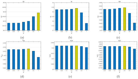
Figure 7.
Influence of parameter on objective metrics. Average values of each metric are obtained via the testing dataset. From left to right for each metric, = 0.01, 0.05, 0.1, 0.3, 0.5, 0.8, and 1. (a) SD, (b) MI, (c) FMI, (d) Q, (e) NCIE, (f) NCC.
(iii) Fusion performance influence of : On the basis of = 0.01 and = 0.5, Figure 8 gives the fusion performance influence of in the range [1, 8]. From Figure 8a,b,d, three metrics SD, MI and Q remain uptrend with the value of increasing and all achieve the highest values at = 8. Moreover, has little effect on NCIE and NCC. The values of NCIE and NCC remain the relatively stable state. Whereas FMI keeps downtrend with the value of increasing and obtains the highest value at = 5. On the one hand, = 6 or 7 reaches a best compromise between = 5 and = 8 for all metrics. On the other hand, (4, 5, 6) has the benefit of taking salient objects/regions in both IR and visible images into account. Therefore, = 6, as an overlap, is selected as the optimal value according to the two above-mentioned concerns.
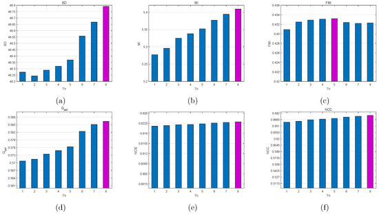
Figure 8.
Influence of parameter on objective metrics. Average values of each metric are obtained via the testing dataset. From left to right for each metric, = 1, 2, 3, 4, 5, 6, 7, and 8. (a) SD, (b) MI, (c) FMI, (d) Q, (e) NCIE, (f) NCC.
Herein, = 0.01, = 0.5, and are set throughout this paper.
5. Results and Analysis
In what follows, extensive experimental results and corresponding analysis are presented via subjective evaluations and objective assessments in Section 5.1 and Section 5.2, respectively.
5.1. Qualitative Analysis via Subjective Evaluations
Figure 9 shows the fusion results of the first three source image pairs ‘Bench’ (S1), ‘Camp’ (S2), and ‘Road’ (S3) in the image dataset. For ‘Bench’ in the first two rows (Figure 9(a1–a12)), the IR image (Figure 9(a1)) clearly gives the person information. However, it lacks texture information of the background. Contrarily, the visible image (Figure 9(a2)) can provide detailed textures of the background. The outputs of DWT, CSR, TSVSM, ResNET, and IFCNN (see the yellow boxes in Figure 9(a3–a5,a8,a9)) suffer from severe contrast distortions, thereby not easily highlighting the targets from the background. VSMWLS, TE, and DDcGAN can achieve a good visual effect of the targeted person. Whereas VSMWLS lacks the detailed texturs (see the yellow boxes in Figure 9(a7)), and there exists brightness loss of the ground in TE and DDcGAN (see the yellow rectangles in Figure 9(a10,a11)). DDcGAN can highlight the person well, but the outline shape is indistinct (see the blue box in Figure 9(a11)) due to the over-enhancement. On the contrary, JSRSD and our method can effectively merge both the targeted information from the IR image without contrast distortions and the background information from the visible image without brightness loss.
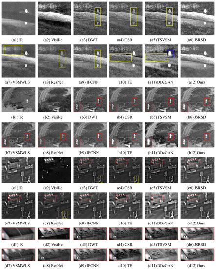
Figure 9.
Fusion performances of various methods (DWT [17], CSR [29], TSVSM [8], JSRSD [30], VSMWLS [27], ResNet [32], IFCNN [36], TE [44], and DDcGAN [37]) on the image pairs. From top to bottom: ‘Bench’ (S1), ‘Camp’ (S2), ‘Road’ (S3), and the close-up views of the fusion results of various methods on ‘Road’. (a1–a12) The source image pair ‘Bench’ (S1) and fusion results of various methods on ‘Bench’, (b1–b12) The source image pair ‘Camp’ (S2) and fusion results of various methods on ‘Camp’, (c1–c12) The source image pair ‘Road’ (S3) and fusion results of various methods on ‘Road’, (d1–d12) The close-up views of the fusion results of various methods on ‘Road’.
As shown in close-up views of ‘Camp’ (S2) (see the red boxes in Figure 9(b1–b12)), there are halo artifacts around the person for DWT (Figure 9(b3)). Moreover, DWT, CSR, and ResNET have low brightness of the person, and an unclear outline shape is similar to Figure 9(a11) in DDcGAN. The results of TSVSM, JSRSD, VSMWLS, IFCNN, TE, and our method fused IR and visible images well. It is hard to judge good from bad for TSVSM, JSRSD, VSMWLS, IFCNN, TE, and our method only on according to visual effects.
Figure 9(c1–c12) illustrates the fusion images of ‘Road’ (S3). Persons and car wheels in Figure 9(c3,c4,c8) suffer from low brightness. Furthermore, Figure 9(d1–d12) displays the close-up view of the billboard ‘NERO’. A number of black stains occur on the billboards of DWT, CSR, TSVSM, JSRSD, VSMWLS, and TE. ResNET (Figure 9(d8)), IFCNN (Figure 9(d9)), and DDcGAN (Figure 9(d11)) cannot maintain brightness well compared with that of the visible image (Figure 9(d2)) and our method (Figure 9(d12)). For the bottom edges of the billboard ‘NERO’, DDcGAN and our method are capable of maintaining edge structures well.
For ‘Sandpath’ (S4, Figure 10(a1–a12)), it is self-evident that the results of DWT, CSR, and ResNet cannot highlight the person due to low brightness (see the yellow rectangle). DWT, CSR, TSVSM, VSMWLS, ResNet, TE, and DDcGAN are not able to merge the visible information well (see the red rectangle). Seeing the top right-hand corner of Figure 10(a6), JSRSD encounters the blocking artifacts whereas important targets/regions were well integrated. Although IFCNN achieves a good performance, our method is visually more pleasing than IFCNN.
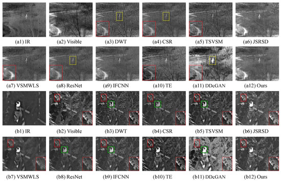
Figure 10.
Fusion performances of various methods (DWT [17], CSR [29], TSVSM [8], JSRSD [30], VSMWLS [27], ResNet [32], IFCNN [36], TE [44], and DDcGAN [37]) on the image pairs. From top to bottom: ‘Sandpath’ (S4) and ‘Garden’ (S5). (a1–a12) The source image pair ‘Sandpath’ (S4) and fusion results of various methods on ‘Sandpath’, (b1–b12) The source image pair ‘Garden’ (S5) and fusion results of various methods on ‘Garden’.
In the eyes of ‘Garden’ (S5, Figure 10(b1–b12)), the targeted persons in Figure 10(b3,b4,b8) are dim (see the green boxes), whereas the person and background suffer from over-enhancement in Figure 10(b11). In the view of detailed textures, all fusion methods have good performances except for VSMWLS (see the leaf in the red box of Figure 10(b7)).
To provide the clear outputs of the test image, we display the fusion results of ‘Tank’ (S6) in a larger size. For ‘Tank’, Figure 11(a1) clearly provides the thermal radiation information of targets (e.g., the tank), but there is no sign of detail information of the trees and the grass. In contrast to the IR image, the visible image (Figure 11(a2)) is capable of providing rich details and textures of the trees and grass, whereas has no abundant detail information of ‘Tank’. For the rear of ‘Tank’ (see the yellow rectangle), DWT, CSR, TSVSM, VSMWLS, ResNet, and IFCNN suffer from contrast distortions, meanwhile JSRSD, TE, DDcGAN and our method are free of this defect. Furthermore, the wheels of ‘Tank’ (see the close-up views in red boxes) have black stains in eight other methods except DDcGAN and our method. For the grass (see the green rectangles), the fusion results of JSRSD and our method look like more clearer and natural than the ones of the rest methods. Therefore, our THPF-VSTO-SR method is effective to integrate the significant and complementary information of IR and visible images into a well-pleasing image.
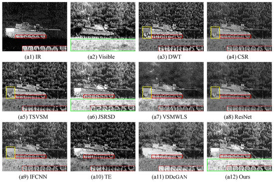
Figure 11.
Fusion performances of various methods (DWT [17], CSR [29], TSVSM [8], JSRSD [30], VSMWLS [27], ResNet [32], IFCNN [36], TE [44], and DDcGAN [37]) on the image pair ‘Tank’ (S6).
In addition, to comprehensively prove the effectiveness of our method, more experiments of 14 other image pairs (S7–S20) are carried out. The performances of various methods on 14 other image pairs are shown in Figure 12. Through comparisons via the experimental results, JSRSD, VSMWLS, IFCNN, TE, DDcGAN and our THPF-VSTO-SR method can achieve good visual performances. Section 5.2 will give the objective evaluation quantitatively.
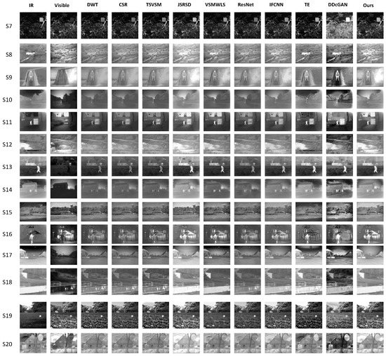
Figure 12.
Fusion performances of various methods (DWT [17], CSR [29], TSVSM [8], JSRSD [30], VSMWLS [27], ResNet [32], IFCNN [36], TE [44], and DDcGAN [37]) on 14 other IR and visible image pairs. Labels for marking each column image are provided in top row. From top to bottom: S7–S20 (‘Square’, ‘Bunker’, ‘Soldier in trench 1’, ‘Movie01’, ‘Kaptein1123’, ‘Lake’, ‘Pedestrian’, ‘Houses with 3 men’, ‘Pancake house’, ‘Kaptein1154’, ‘Marne 03’, ‘Wall’, ‘Square3’, and ‘Man in door way’).
5.2. Quantitative Analysis via Objective Assessments
Figure 13 presents quantitative comparisons of evaluation metrics (SD, MI, FMI, Q, NCIE, and NCC) using nine representative methods on 20 image pairs. Our THPF-VSTO-SR method outperforms nine other methods on MI, Q, NCIE, and NCC and achieves nearly all the best values on the metrics FMI and Q. On the whole, THPF-VSTO-SR has substantial advantages on MI, NCIE, and NCC. Our proposed method leads narrowly on FMI and Q on the image pairs whereas nine other methods also work well. DDcGAN has superiority on SD, while JSRSD and our method also have good results in most samples.
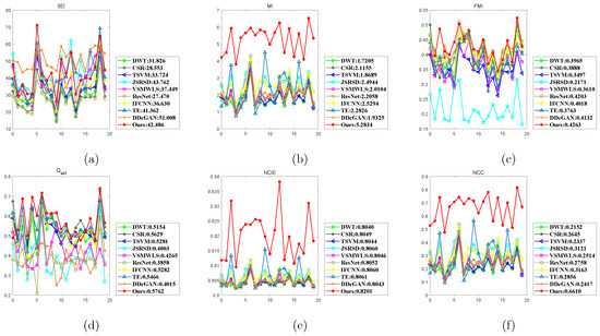
Figure 13.
Quantitative comparisons of 4 metrics using various representative methods (DWT [17], CSR [29], TSVSM [8], JSRSD [30], VSMWLS [27], ResNet [32], IFCNN [36], TE [44], and DDcGAN [37]) on 20 IR and visible image pairs. For all methods, the average values are provided in the legend. From 0 to 19: S1–S20. (a) SD, (b) MI, (c) FMI, (d) Q, (e) NCIE, (f) NCC.
For all methods, the average values of SD, MI, FMI, Q, NCIE, and NCC on 20 image pairs are given in the legend of Figure 13 and specially shown in Table 1 for the sake of observation and comparison, respectively. The highest value standing for the best performance is highlighted in ’red’ for each metric. Accordingly, the second best value is highlighted in ’green’, and the third best value is highlighted in ’blue’.

Table 1.
Average values of each metric for 20 source image pairs of various fusion methods.
From Table 1, all average metric values of our THPF-VSTO-SR method outperform the ones of other nine state-of-the-art methods, except for SD. For SD in Table 1, DDcGAN achieves the highest score but the outline distortions of targets arise out of the over-enhancement in the fused images (e.g., Figure 9(a11,b11)). Objectively, the targets/regions in the fusion results of JSRSD and our method are natural and pleasing in most cases, and the values of SD between JSRSD and our method are with a very small difference. JSRSD, IFCNN, ResNet, CSR, TE and IFCNN are the runners-up on SD, MI, FMI, Q, NCIE, and NCC, respectively. Besides, our method, JSRSD, DDcGAN, TE, JSRSD in a tie with IFCNN, and JSRSD win the third place on SD, MI, FMI, Q, NCIE, and NCC, respectively. Except for the champion THPF-VSTO-SR, CSR, ResNet, IFCNN, TE, JSRSD, and DDcGAN also earn a fairly good competition outcome via objective assessments, respectively.
Through the qualitative analysis and the quantitative analysis, extensive experimental results suggest that our THPF-VSTO-SR scheme achieves better performances than other representative methods.
5.3. Running Time Comparison
Table 2 provides the average running time of various methods tested on ’Camp’ (S2) with the size 270 × 360. From Table 2, the computational efficiency of our method is not as high as DWT, TSVSM, VSMWLS, ResNet, IFCNN, and TE because of consuming a large amount of time with huge-scale data processing using sparse coding. IFCNN wins the first place with the help of GPU. Whereas THPF-VSTO-SR has less running time than CSR and JSRSD. The running time of sparse representation based methods is longer than most of multiscale decomposition and the spatial transform based fusion methods. But more importantly, the presented method achieves a comparable or superior performance in comparison with several state-of-the-art methods in the fusion performance. In addition, the random access memory resources of the fusion methods respectively require 4258M, 4414M, 4275M, 4470M, 4451M, 4401M, 5164M, 4259M, 5249M, and 4175M.
Table 2.
Average running time of various methods tested on ’Camp’ (S2) with size 270 × 360 (Unit: s).
6. Conclusions and Future Work
This paper proposes a novel image fusion method for infrared and visible images using truncated Huber penalty function (THPF) smoothing based image decomposition, visual saliency based threshold optimization (VSTO) fusion strategy, and sparse representation (SR) fusion strategy. In the presented THPF-VSTO-SR method, source images are decomposed into the approximate layer images and residual layer images. For approximate layer components, a visual saliency based threshold optimization fusion rule is proposed aiming to highlight the significant targets/regions in both infrared and visible images. For residual layer components, sparse representation based fusion scheme is implemented with the goal of capturing the intrinsic structure and texture information. Extensive experimental results demonstrate that the proposed THPF-VSTO-SR method can achieve a comparable or superior performance compared with several state-of-the-art fusion methods via subjective evaluations and objective assessments.
However, the proposed THPF-VSTO-SR method has a few limitations: (i) The computational efficiency of our method is lower than most of traditional multiscale decomposition and spatial transform based fusion methods (i.e., DWT, TSVSM, VSMWLS, and TE). The reason is twofold: considerable matrix computations in sparse dictionary coding of our method, and simple and fast fusion rules in traditional methods. (ii) The advantages of THPF-VSTO-SR is only demonstrated by infrared and visible images. Other modality images, such as remote sensing images, multifocus images, medical images, are not taken into account using our method. Therefore, there are some concerns to be worth investigating in following work. For the first limitation, we can try to use multithread computing and GPU to boost the huge-scale data computations in SR-based fusion methods. The second can be solved by exploring fast and efficient fusion rules to reduce the computational time. Besides, we will also devote to investigate the general frameworks for simultaneously merging different multimodality images.
Author Contributions
Conceptualization, C.D. and C.X.; methodology, C.D., C.X. and Z.W.; software, C.D. and Y.L.; validation, C.D. and C.X.; formal analysis, C.D. and C.X.; investigation, C.D. and C.X.; resources, Y.L. and Z.W.; data curation, C.D. and Y.L.; writing—original draft preparation, C.D.; writing—review and editing, C.X., Y.L. and Z.W.; visualization, C.X. and Y.L.; supervision, Z.W.; project administration, Z.W.; funding acquisition, Z.W., C.X. and C.D. All authors have read and agreed to the published version of the manuscript.
Funding
This research was funded by National Natural Science Foundation of China [grant no. 62101247 and 62106104], Special Fund for Guiding Local Scientific and Technological Development of the Central Government in Shenzhen [grant no. 2021Szvup063], and Aeronautical Science Foundation of China [grant no. 20162852031].
Institutional Review Board Statement
A study involving humans or animals is absent.
Informed Consent Statement
A study involving humans is absent.
Conflicts of Interest
The authors declare no conflict of interest.
References
- Yang, Y.; Zhang, Y.; Huang, S.; Zuo, Y.; Sun, J. Infrared and Visible Image Fusion Using Visual Saliency Sparse Representation and Detail Injection Model. IEEE Trans. Instrum. Meas. 2021, 70, 1–15. [Google Scholar] [CrossRef]
- Ma, J.; Ma, Y.; Li, C. Infrared and visible image fusion methods and applications: A survey. Inf. Fusion 2019, 45, 153–178. [Google Scholar] [CrossRef]
- Hou, J.; Zhang, D.; Wu, W.; Ma, J.; Zhou, H. A Generative Adversarial Network for Infrared and Visible Image Fusion Based on Semantic Segmentation. Entropy 2021, 23, 376. [Google Scholar] [CrossRef] [PubMed]
- Li, S.; Kang, X.; Fang, L.; Hu, J.; Yin, H. Pixel-level image fusion: A survey of the state of the art. Inf. Fusion 2017, 33, 100–112. [Google Scholar] [CrossRef]
- Zhang, S.; Liu, F. Infrared and visible image fusion based on non-subsampled shearlet transform, regional energy, and co-occurrence filtering. Electron. Lett. 2020, 56, 761–764. [Google Scholar] [CrossRef]
- Jin, X.; Qian, J.; Yao, S.; Zhou, D.; He, K. A survey of infrared and visual image fusion methods. Infrared Phys. Technol. 2017, 85, 478–501. [Google Scholar] [CrossRef]
- Liu, L.; Chen, M.; Xu, M.; Li, X. Two-stream network for infrared and visible images fusion. Neurocomputing 2021, 460, 50–58. [Google Scholar] [CrossRef]
- Bavirisetti, D.P.; Dhuli, R. Two-scale image fusion of visible and infrared images using saliency detection. Infrared Phys. Technol. 2016, 76, 52–64. [Google Scholar] [CrossRef]
- Liu, Y.; Chen, X.; Wang, Z.; Wang, Z.; Ward, R.K.; Wang, X. Deep learning for pixel-level image fusion: Recent advances and future prospects. Inf. Fusion 2018, 42, 158–173. [Google Scholar] [CrossRef]
- Zhang, Q.; Liu, Y.; Blum, R.S.; Han, J.; Tao, D. Sparse representation based multi-sensor image fusion for multi-focus and multi-modality images: A review. Inf. Fusion 2018, 40, 57–75. [Google Scholar] [CrossRef]
- Sun, C.; Zhang, C.; Xiong, N. Infrared and Visible Image Fusion Techniques Based on Deep Learning: A Review. Electronics 2020, 9, 2162. [Google Scholar] [CrossRef]
- Zhang, Z.; Blum, R.S. A categorization of multiscale-decomposition-based image fusion schemes with a performance study for a digital camera application. Proc. IEEE 1999, 87, 1315–1326. [Google Scholar] [CrossRef] [Green Version]
- Meher, B.; Agrawal, S.; Panda, R.; Abraham, A. A survey on region based image fusion methods Information Fusion. Inf. Fusion 2019, 48, 119–132. [Google Scholar] [CrossRef]
- Patel, A.; Chaudhary, J. A Review on Infrared and Visible Image Fusion Techniques. In Intelligent Communication Technologies and Virtual Mobile Networks; Balaji, S., Rocha, A., Chung, Y., Eds.; Springer: Cham, Switzerland, 2020; pp. 127–144. [Google Scholar]
- Ji, L.; Yang, F.; Guo, X. Image Fusion Algorithm Selection Based on Fusion Validity Distribution Combination of Difference Features. Electronics 2021, 10, 1752. [Google Scholar] [CrossRef]
- Burt, P.J.; Adelson, E.H. The laplacian pyramid as a compact image code. IEEE Trans. Commun. 1983, 31, 532–540. [Google Scholar] [CrossRef]
- Li, H.; Manjunath, B.; Mitra, S. Multisensor image fusion using the wavelet transform. Graph. Models Image Process. 1995, 57, 235–245. [Google Scholar] [CrossRef]
- Lewis, J.J.; O’Callaghan, R.J.; Nikolov, S.G.; Bull, D.R.; Canagarajah, N. Pixel- and region-based image fusion with complex wavelets. Inf. Fusion 2007, 8, 119–130. [Google Scholar] [CrossRef]
- Nencini, F.; Garzelli, A.; Baronti, S.; Alparone, L. Remote sensing image fusion using the curvelet transform. Inf. Fusion 2007, 8, 143–156. [Google Scholar] [CrossRef]
- Do, M.N.; Vetterli, M. The Contourlet transform: an efficient directional multiresolution image representation. IEEE Trans. Image Process. 2005, 14, 2091–2106. [Google Scholar] [CrossRef] [Green Version]
- Zhang, Q.; Guo, B. Multifocus image fusion using the nonsubsampled Contourlet transform. Signal Process. 2009, 89, 1334–1346. [Google Scholar] [CrossRef]
- Yazdi, M.; Ghasrodashti, E.K. Image fusion based on Non-Subsampled Contourlet Transform and phase congruency. In Proceedings of the 2012 19th International Conference on Systems, Signals and Image Processing (IWSSIP), Vienna, Austria, 11–13 April 2012; pp. 616–620. [Google Scholar]
- Kong, W.; Wang, B.; Lei, Y. Technique for infrared and visible image fusion based on non-subsampled shearlet transform and spiking cortical model. Infrared Phys. Technol. 2015, 71, 87–98. [Google Scholar] [CrossRef]
- Li, S.; Kang, X.; Hu, J. Image fusion with guided filtering. IEEE Trans. Image Process. 2013, 22, 2864–2875. [Google Scholar] [PubMed]
- Kumar, B.K.S. Image fusion based on pixel significance using cross bilateral filter. Signal Image Video Process. 2015, 9, 1193–1204. [Google Scholar] [CrossRef]
- Zhou, Z.; Wang, B.; Li, S.; Dong, M. Perceptual fusion of infrared and visible images through a hybrid multiscale decomposition with Gaussian and bilateral filters. Inf. Fusion 2016, 30, 15–26. [Google Scholar] [CrossRef]
- Ma, J.; Zhou, Z.; Wang, B.; Zong, H. Infrared and visible image fusion based on visual saliency map and weighted least square optimization. Infrared Phys. Technol. 2017, 82, 8–17. [Google Scholar] [CrossRef]
- Liu, Y.; Liu, S.; Wang, Z. A general framework for image fusion based on multiscale transform and sparse representation. Inf. Fusion 2015, 24, 147–164. [Google Scholar] [CrossRef]
- Liu, Y.; Chen, X.; Ward, R.K.; Wang, Z. Image Fusion with Convolutional Sparse Representation. IEEE Signal Process. Let. 2016, 23, 1882–1886. [Google Scholar] [CrossRef]
- Liu, C.; Qi, Y.; Ding, W. Infrared and visible image fusion method based on saliency detection in sparse domain. Infrared Phys. Technol. 2017, 83, 94–102. [Google Scholar] [CrossRef]
- Ma, T.; Jie, M.; Fang, B.; Hu, F.; Quan, S.; Du, H. Multi-scale decomposition based fusion of infrared and visible image via total variation and saliency analysis. Infrared Phys. Technol. 2018, 92, 154–162. [Google Scholar] [CrossRef]
- Li, H.; Wu, X.J.; Durrani, T.S. Infrared and Visible Image Fusion with ResNet and zero-phase component analysis. Infrared Phys. Technol. 2019, 102, 103039. [Google Scholar] [CrossRef] [Green Version]
- Liu, Y.; Chen, X.; Cheng, J.; Peng, H.; Wang, Z. Infrared and visible image fusion with convolutional neural networks. Int. J. Wavelets Multiresolution Inf. Process. 2018, 16, 353–389. [Google Scholar] [CrossRef]
- Liu, Y.; Dong, L.; Ji, Y.; Xu, W. Infrared and Visible Image Fusion through Details Preservation. Sensors 2019, 19, 4556. [Google Scholar] [CrossRef] [Green Version]
- An, W.; Wang, H. Infrared and visible image fusion with supervised convolutional neural network. Optik 2020, 219, 165120. [Google Scholar] [CrossRef]
- Zhang, Y.; Liu, Y.; Sun, P.; Yan, H.; Zhao, X.; Zhang, L. IFCNN: A general image fusion framework based on convolutional neural network. Inf. Fusion 2020, 54, 99–118. [Google Scholar] [CrossRef]
- Ma, J.; Xu, H.; Jiang, J.; Mei, X.; Zhang, X. DDcGAN: A Dual-Discriminator Conditional Generative Adversarial Network for Multi-Resolution Image Fusion. IEEE Trans. Image Process. 2020, 29, 4980–4995. [Google Scholar] [CrossRef] [PubMed]
- Liu, W.; Zhang, P.; Lei, Y.; Huang, X.; Reid, I. A generalized framework for edge-preserving and structure-preserving image smoothing. IEEE Trans. Pattern Anal. Mach. Intell. 2021. [Google Scholar] [CrossRef] [PubMed]
- Huber, P.J. Robust estimation of a location parameter. The Annals of Mathematical Statistics. Ann. Math. Stat. 1964, 35, 73–101. [Google Scholar] [CrossRef]
- Ghasrodashti, E.K.; Karami, A.; Heylen, R.; Scheunders, P. Spatial Resolution Enhancement of Hyperspectral Images Using Spectral Unmixing and Bayesian Sparse Representation. Remote Sens. 2017, 9, 541. [Google Scholar] [CrossRef] [Green Version]
- Ghasrodashti, E.K.; Helfroush, M.S.; Danyali, H. Sparse-Based Classification of Hyperspectral Images Using Extended Hidden Markov Random Fields. IEEE J.-STARS 2018, 11, 4101–4112. [Google Scholar] [CrossRef]
- Bruckstein, A.M.; Donoho, D.L.; Elad, M. From sparse solutions of systems of equations to sparse modeling of signals and images. SIAM Rev. 2009, 51, 34–81. [Google Scholar] [CrossRef] [Green Version]
- Aharon, M.; Elad, M.; Bruckstein, A. K-SVD: An Algorithm for Designing Overcomplete Dictionaries for Sparse Representation. IEEE Trans. Image Process. 2006, 54, 4311–4322. [Google Scholar] [CrossRef]
- Chen, J.; Li, X.; Luo, L.; Mei, X.; Ma, J. Infrared and visible image fusion based on target-enhanced multiscale transform decomposition. Inf. Sci. 2020, 508, 64–78. [Google Scholar] [CrossRef]
- Qu, G.; Zhang, D.; Yan, P. Information measure for performance of image fusion. Inf. Sci. 2002, 38, 313–315. [Google Scholar] [CrossRef] [Green Version]
- Haghighat, M.B.A.; Aghagolzadeh, A. A non-reference image fusion metric based on mutual information of image featuresn. Comput. Electr. Eng. 2011, 37, 744–756. [Google Scholar] [CrossRef]
- Xydeas, C.S.; Petrovic, V. Objective image fusion performance measure. Electron. Lett. 2000, 36, 308–309. [Google Scholar] [CrossRef] [Green Version]
- Wang, Q.; Shen, Y.; Zhang, J.Q. A nonlinear correlation measure for multivariable data set. Phys. D Nonlinear Phenom. 2005, 200, 287–295. [Google Scholar] [CrossRef]
- Liu, Z.; Blasch, E.; Xue, Z.; Zhao, J.; Laganiere, R.; Wu, W. Objective Assessment of Multiresolution Image Fusion Algorithms for Context Enhancement in Night Vision: A Comparative Study. IEEE Trans. Pattern Anal. Mach. Intell. 2012, 34, 94–109. [Google Scholar] [CrossRef] [PubMed]
- Wang, Q.; Shen, Y.; Jin, J. Performance evaluation of image fusion techniques. In Image Fusion: Algorithms and Applications; Stathaki, T., Ed.; Academic Press: Oxford, UK; Orlando, FL, USA, 2008; pp. 469–492. [Google Scholar]
Publisher’s Note: MDPI stays neutral with regard to jurisdictional claims in published maps and institutional affiliations. |
© 2021 by the authors. Licensee MDPI, Basel, Switzerland. This article is an open access article distributed under the terms and conditions of the Creative Commons Attribution (CC BY) license (https://creativecommons.org/licenses/by/4.0/).