The Role of Genetic Algorithm Selection Operators in Extending WSN Stability Period: A Comparative Study

Abstract

A genetic algorithm (GA) contains a number of genetic operators that can be tweaked to improve the performance of specific implementations. Parent selection, crossover, and mutation are examples of these operators. One of the most important operations in GA is selection. The performance of GA in addressing the single-objective wireless sensor network stability period extension problem using various parent selection methods is evaluated and compared. In this paper, six GA selection operators are used: roulette wheel, linear rank, exponential rank, stochastic universal sampling, tournament, and truncation. According to the simulation results, the truncation selection operator is the most efficient operator in terms of extending the network stability period and improving reliability. The truncation operator outperforms other selection operators, most notably the well-known roulette wheel operator, by increasing the stability period by $25.8\%$ and data throughput by $26.86\%$. Furthermore, the truncation selection operator outperforms other selection operators in terms of the network residual energy after each protocol round.

1. Introduction

As a result of rapid advancements in the field of micro-electro-mechanical systems (MEMS), small sensor nodes have become inexpensive and self-sufficient [1]. These sensor nodes can sense and monitor the environment, analyze and aggregate data, and communicate data to one other or to a central point, commonly known as the sink. Sensor nodes can be interconnected to serve an application-specific purpose through the use of wireless sensor networks (WSN) [2,3].

Sensor nodes have a certain amount of battery power, and these batteries are rarely rechargeable. Sensor nodes often use the most energy for their communication functions [4]. When a node’s energy source runs out, the node is declared dead and is no longer useful. WSNs can be used in a wide variety of real-world situations. They are employed in a variety of fields, including agriculture, industry, health care, surveillance, target tracking, and security management, in both the civilian and military sectors [5,6,7]. 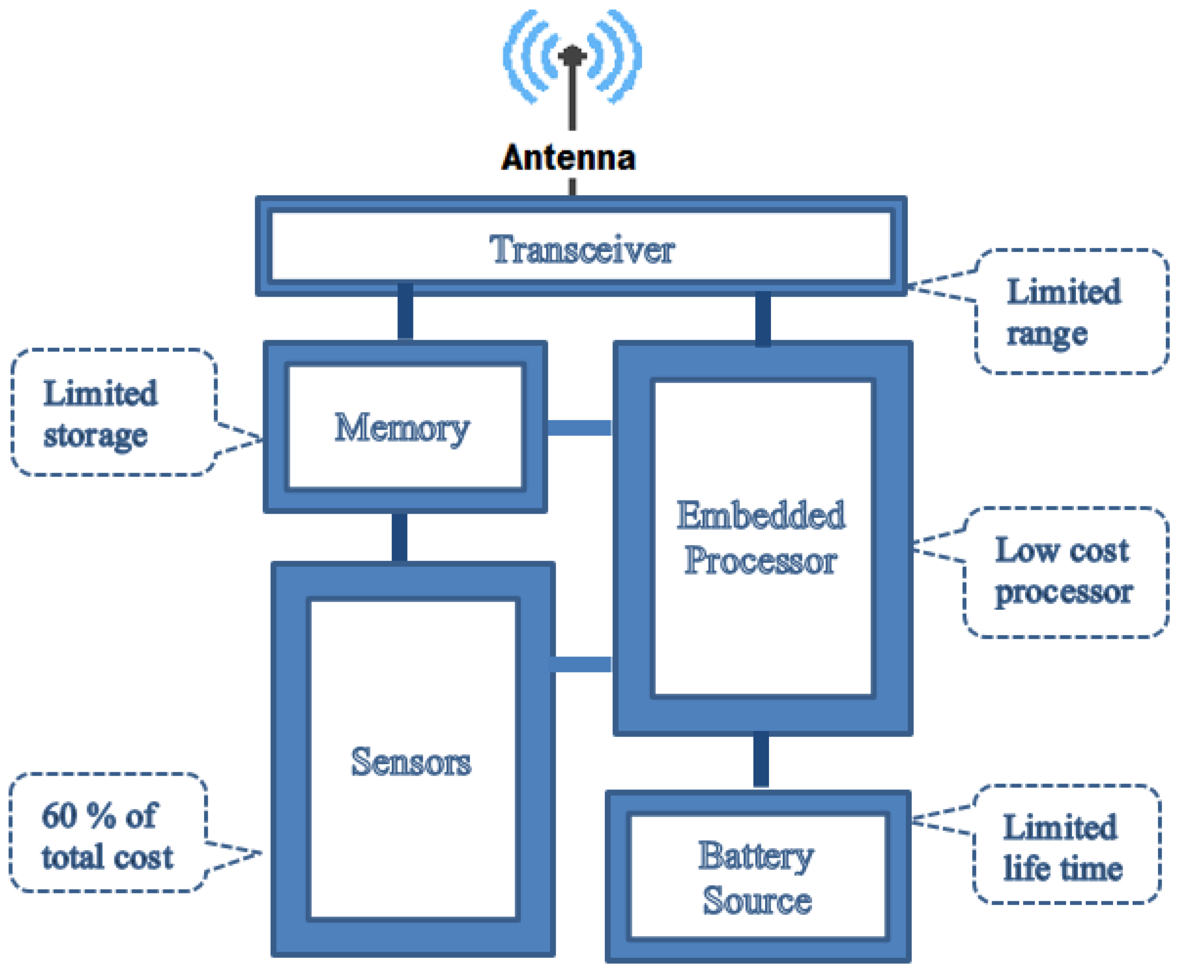Figure 1 shows a typical sensor node block diagram [8].

Sensor nodes have the ability to send their collected data straight to the sink node [9], but this consumes more energy and leads to the premature death of the node; as a result, other issues are introduced into the network, such as the coverage/hole problem [10]. Using clustering, sensor nodes can be balanced in terms of energy consumption. Clustering is based on putting together nodes that are near each other or have similar characteristics or functions. Cluster heads (CH) and member nodes (MN) are the two types of nodes that make up a cluster. MNs gather information from the environment and send it to the CH. Additionally, CHs collect, compress, and send data to the sink node.

Direct communication between CH and sink node is possible, as well as communication involving multiple hops [11]. In general, CHs use more energy than MNs. The CH role must be rotated between network nodes in order to maintain a stable overall network energy level while also extending the network’s life span [12]. For the creation, operation, and maintenance of clusters, numerous protocols have been designed. A number of them, such as low energy adaptive clustering hierarchy (LEACH) and stable election protocol (SEP), can be found in the literature [13]. Clustering and routing protocols in WSNs have a problem in that they cannot reduce the overall network energy and balance energy consumption among sensor nodes over the network’s lifetime [11]. In some cases, a significant reduction in the overall energy consumption of the network is achieved at the expense of unequal remaining energies among sensor points. In other cases, balancing the remaining energies of sensor nodes is achieved at the expense of increasing the overall energy consumed by the network.

WSNs use meta-heuristics algorithms, which are also known as nature-inspired algorithms, or intelligent optimization algorithms, to balance energy consumption among sensor nodes while also reducing overall energy consumption [14,15]. This trade-off has proven to be successful. There are four types of meta-heuristic algorithms: bio-inspired, human-inspired, geography-inspired, and physics-inspired. The biological system is the source of inspiration for the vast majority of nature-inspired algorithms. The bio-inspired algorithms are further classified into three categories, namely evolutionary, swarm-based and plant-based [16,17]. The genetic algorithm (GA) is a meta-heuristic, bio-inspired and evolutionary technique, which is widely used in WSNs to solve fundamental problems, such as sensor node localization, energy efficient clustering, data aggregation and optimal coverage [18]. With GA, the number of clusters in the network can be optimized, and sensor node energy consumption can be balanced, allowing the WSN to operate for longer time periods. In lieu of two-dimensional WSN (2D-WSN), three-dimensional WSN (3D-WSN) is being researched because it is more realistic than 2D-WSN since the third dimension is crucial in determining the WSN’s lifespan [5].

GA is made up of three main components: selection, crossover, and mutation. The selection operator is responsible for the production of the next generation; crossover and mutation are responsible for the manipulation of the selected individuals to form the next generation. The mechanism of selection determines which individuals are selected for reproduction (mating) and how many offspring each selected individual produces. The selection strategy’s core principle is that the better an individual is, the greater the likelihood that it will be a parent. As a rule of thumb, crossover and mutation expand the search area, while selection narrows the search area within a population by eliminating poor solutions [19].

This study has the following contributions: First, the central dynamic clustering protocol based on GA for extending the 3D WSN stability period is proposed. Second, six GA selection operators are utilized, evaluated and compared for better reliability and maximum network life time. Three, a new GA fitness function is used to optimize the number of clusters in the network, which essentially includes information about the type of connections that MNs establish with CHs in a cluster and CHs establish with the sink in the network.

The rest of the paper is organized as follows: Section 2 overviews the related work. Section 3 describes the GA operators’ details. In Section 4, the simulation setup and configuration are provided. The simulation results are explained in Section 5. Finally, we conclude our research and provide some future work in Section 6.

2. Related Work

Energy conservation in WSN is critical for extending the lifetime and ensuring the smooth operation of resource-constrained nodes in the network. Many techniques are proposed in the literature to increase the lifespan and reliability of WSNs. Clustering/routing, mobile relays and sinks, optimal node deployment, data correlation, energy harvesting, beamforming, and various optimization techniques are among them [20,21]. In the following sections, we limit our related work to optimization techniques that use nature-inspired algorithms, specifically the GA. There are numerous studies that used meta-heuristic algorithms to extend the life of WSNs. GA has demonstrated a wide range of applicability and solutions in WSNs. An energy-efficient clustering protocol (GAEEC) was proposed by the authors in [22], which divided the network into optimal numbers of clusters using GA before using GA again to select the appropriate node within a cluster as a CH, depending on its fitness function per algorithm round. They found that their protocol outperformed the current renowned LEACH protocol in terms of network throughput and stability. The authors in [23] proposed GAECH, a GA-based energy-efficient clustering hierarchy protocol whose goal is to reduce overall network energy consumption while also extending the network’s lifespan. When the sink node is located outside the network area, their results show a significant increase in network life time compared to other well-known clustering protocols. Using genetic algorithms for energy-efficient clustering and routing in 3D WSNs, the authors in [8] proposed PEGASIS protocol variants. GA was used to create data transmission chains with a remarkably short overall length. An improved method for devising CHs that takes distance and remaining energy into account was developed. Their results showed that the normal PEGASIS protocol was superior in terms of the first-node-die (FND) metric, compared to other well-known protocols. The fuzzy C-means genetic algorithm (FCM-GA) protocol was proposed by the authors in [24]. Two phases make up the protocol. First, clustering is done using FCM based on three objectives: the appropriate distribution of online energy among each cluster, the distances within each cluster, and the separation between each CH and the sink. As compared to other protocols, such as direct transmission, SH-MEER, and MH-FEER, the FCM-GA results show significant gains in terms of both network throughput and life span. In [25], the authors proposed an improved version of the LEACH protocol (O-LEACH). When determining the best route, O-LEACH relies on GA for selecting the best route. As a result, their energy usage was reduced by $17.40\%$.

To the best of our knowledge, no research has been done on the impact of using different GA selection operators on 3D-WSN reliability, lifetime and energy conservation. The following studies looked at and compared the outcomes of using GA selection operators in other domains. Using different parent selection strategies, the authors in [26] compared the GA’s performance in solving the traveling salesman problem (TSP). The results show that the tournament selection strategy outperforms proportional roulette wheel and rank-based roulette wheel selections, achieving the best solution quality with the lowest computing times, in several TSP tests. The results also show that tournament and proportional roulette wheel selection can be superior to rank-based roulette wheel selection only for smaller problems and can become susceptible to premature convergence as the problem size increases. To solve the network topology design problem, the authors in [27] employed three different selection strategies: tournament, ranking, or the use of a roulette wheel. They were compared in terms of quality of solution and computation time. For a 10-node network, tournament selection yielded the best solution in terms of quality and computation time, while ranking and scaling delivered the worst solution in terms of quality and computation time. The solution quality of ranking and scaling was equal to that of tournament selection for networks with 21 and 36 nodes, but tournament outperformed ranking and scaling when it came to computation time.

3. Genetic Algorithm Overview

GA is a stochastic, meta-heuristic optimization algorithm. GA is made up of three different operators: selection, crossover, and mutation. The GA solution is encoded in a binary string known as chromosome. The elements of a chromosome are referred to as genes. The number of genes on each chromosome should be the same. An objective function is used to assess a chromosome’s fitness value. The term population refers to a grouping of chromosomes [19].

GA is an iterative process. It uses the three operators at each run to find new chromosomes that may produce a better solution; see Algorithm 1. The GA operators are as follows:

• Selection operator: Parents with higher fitness values are chosen to produce the next generation’s offspring. Some examples of selection operators include roulette wheel, tournament, and stochastic universal sampling.
• Crossover operator: To produce new offspring, the genes of the two chosen parents are merged. In this phase, uniform-point, single-point, and double-point methods are used separately or collectively.
• Mutation operator: To diversify the search space, single or multiple gene modifications are applied to newly produced chromosomes.

Algorithm 1 shows a typical execution of a simple GA.

Algorithm 1 Simple GA process.

1: Set parameters 2: Choose encode method 3: Generate the initial population 4: while$i<MaxIter$ & $Bestfitness<Maxfitness$ do 5:    Fitness calculation 6:    Selection 7:    Crossover 8:    Mutation 9: end while 10: Decode the individual with max. fitness 11: Return the best solution

The selection operator has the most effect in directing the GA toward the optimal solution and narrowing the search space. Moreover, it aims to exploit the best characteristics of good candidate solutions in order to improve these solutions over generations. This should, in theory, guide the GA to converge to an acceptable and satisfactory solution of the optimization problem at hand. However, despite decades of research, there are no general guidelines or theoretical support for how to choose a good selection method for each problem. This can be a serious issue because a poor selection operator can lead to poor performance of the GA in terms of both speed and reliability [28].

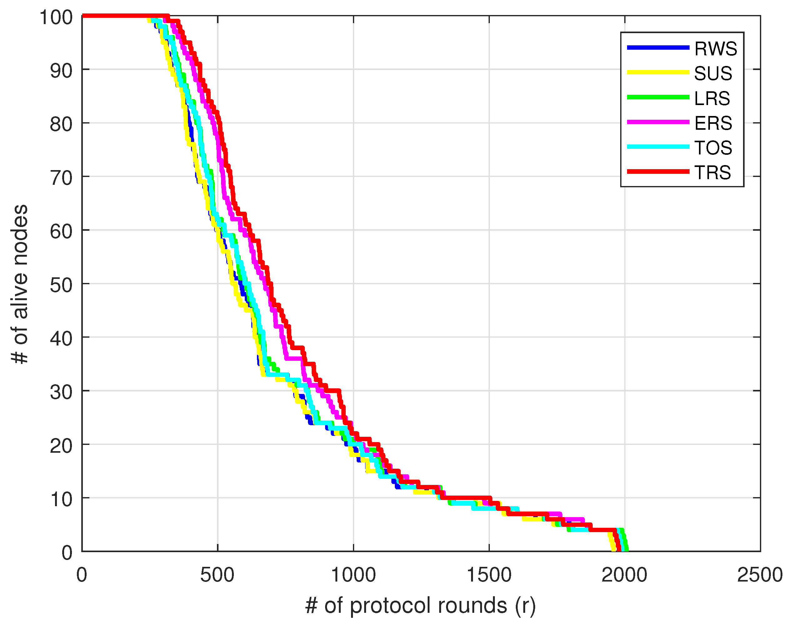
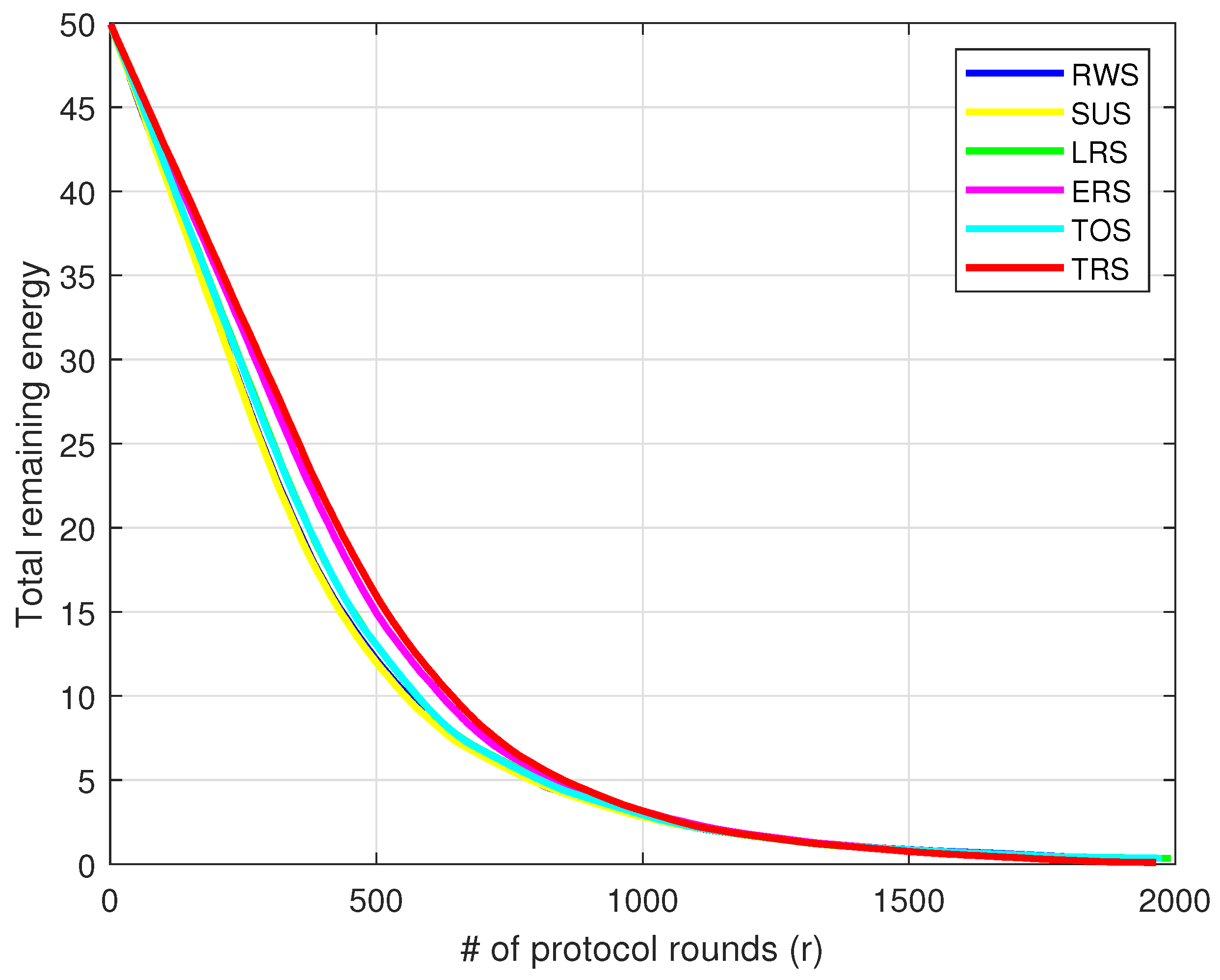
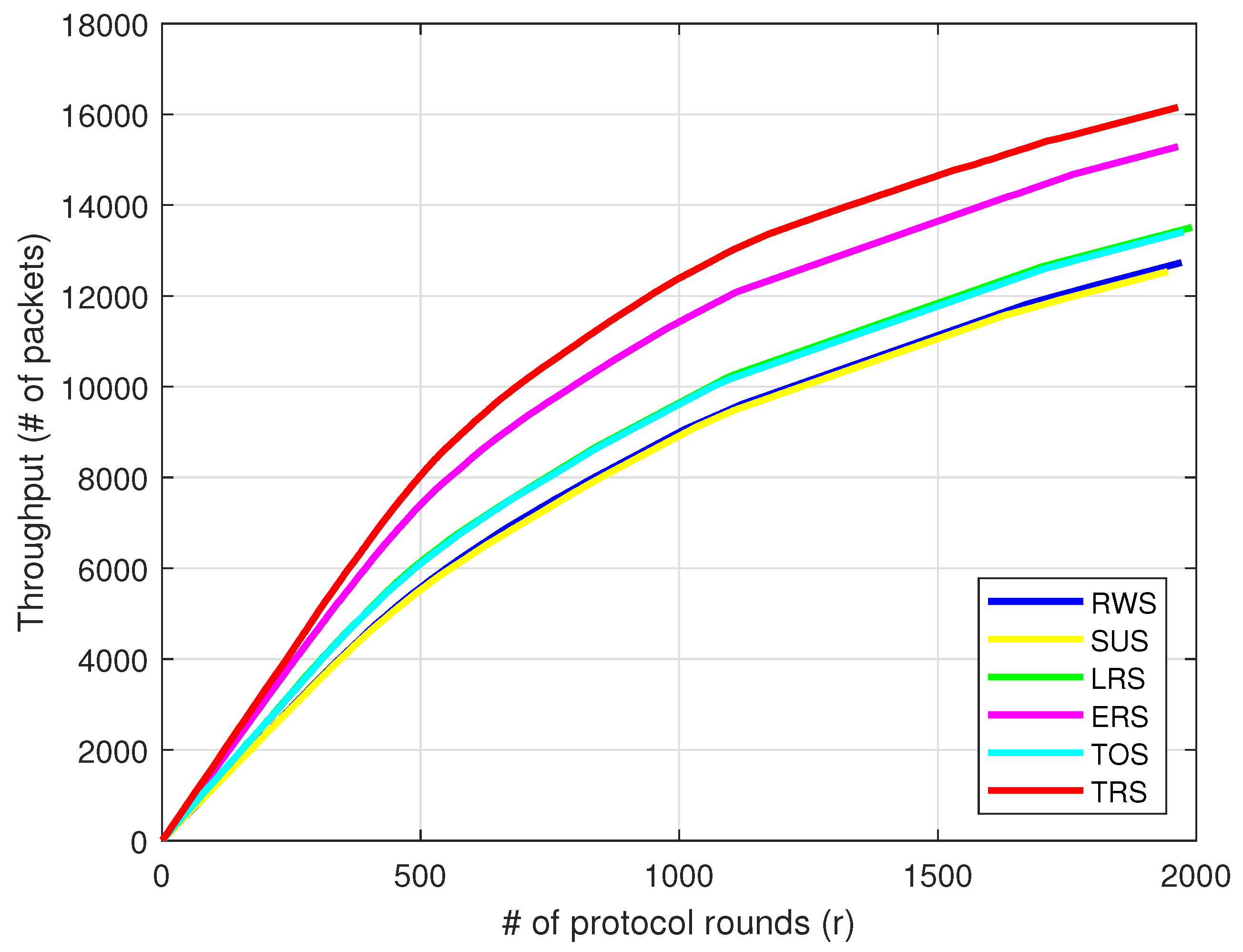
Six different selection operators are utilized in this research to evaluate the performance of 3D WSN, namely [19]: the roulette wheel selection (RWS), the linear rank selection (LRS), the exponential rank selection (ERS), the stochastic universal sampling (SUS), the tournament selection (TOS), and the truncation selection (TRS). All of the algorithms steps are shown in MATLAB as pseudo-code.

• Roulette wheel selection (RWS): The distinguishing feature of this selection method is that it assigns a probability $p_i$ of selection to each chromosome i in the current population, proportional to its fitness value $f_i$ as shown in the following expression.

  $$p_i=\frac{f_i}{{\sum }_{k=1}^n{f}_k}$$

  (1)
  The population size is denoted by n. Algorithm 2 shows the RWS pseudo-code.
  It should be noted that a well-known disadvantage of this technique is the risk of the GA converging to a local optimum too soon, due to the presence of a dominant individual who always wins the competition and is chosen as a parent.
• Linear rank selection (LRS): This is variant of RWS that attempts to overcome the disadvantage of the premature convergence of the GA to a local optimum. It is based on a chromosome’s rank rather than its fitness. The best chromosome receives rank n, while the worst individual receives rank 1. As a result, each chromosome has the probability of being chosen given by the following expression:

  $$p_i=\frac{rank\left(i\right)}{n\ast (n-1)}$$

  (2)
  Algorithm 3 shows the LRS pseudo-code.
• Exponential rank selection (ERS): It is based on the same principle as the LRS, but it varies slightly from the LRS in terms of the probability of selecting each individual. This probability is given by the expression

  $$p_i=\frac{w^{n-i}}{{\sum }_{k=1}^n{w}^{n-k}}$$

  (3)

  where w is the exponent base, a typical value of $w\in \left[01\right]$. Algorithm 4 shows the ERS pseudo-code.
• Stochastic universal sampling (SUS): SUS is roughly equivalent to RWS. The only difference is that instead of a single fixed point, we have several fixed points. As a result, all of the parents are chosen at random from a single spin of the wheel based on their fitness value. Furthermore, such a setup encourages the most highly fit chromosome to be chosen at least once in a spin. Algorithm 5 shows the SUS pseudo-code.
• Tournament selection (TOS): This is a type of ranking-based selection method. Its basic idea is to pick a group of k chromosomes at random. These chromosomes are then ranked based on their relative fitness, with the fittest being chosen for reproduction. TOS is a popular method of selection in evolutionary algorithms. It works well for a wide range of problems, it is easy to implement, and it is parallelizable. Algorithm 6 shows the TOS pseudo-code.
• Truncation selection (TRS): The TRS method sorts chromosomes based on their fitness value. Only the best chromosomes are chosen to be the parents of the next new population. The main parameter for truncation selection is the TRS threshold. It denotes the specified proportion of the population to be chosen as parents, with values ranging from $50\%$ to $10\%$. Individuals who fall below the TRS threshold do not reproduce and are discarded. Algorithm 7 shows the TRS pseudo-code.

Algorithm 2 GA RWS technique.

1: n: number of chromosomes in the population 2: c: vector of chromosomes’ fitness values 3: $cSum=sum\left(c\right)$ 4: $prob=c/cSum$ 5: $pSum=sum\left(prob\right)$ 6: $[pValues,pIndx]=sort\left(prob{,}^{\prime }descen{d}^{\prime }\right)$ 7: $pCumSum=cumsum\left(pValues\right)$ 8: $rnd=pSum\ast rand\left(\right)$                                         ▹$rnd\in \left[01\right]$ 9: $idx=find(rnd\le pCumSum{,}^{\prime }firs{t}^{\prime })$ 10: $returnpIndx\left(idx\right)$

Algorithm 3 GA LRS technique.

1: n: number of chromosomes in the population 2: c: vector of chromosomes’ fitness values 3: $rank=n:-1:1$                                          ▹ vector of ranks 4: $prob=rank/(n\ast (n-1\left)\right)$ 5: $pSum=sum\left(prob\right)$ 6: $[\sim ,fitIndx]=sort\left(c{,}^{\prime }descen{d}^{\prime }\right)$ 7: $pCumSum=cumsum\left(prob\right)$ 8: $rnd=pSum\ast rand\left(\right)$ 9: $idx=find(rnd\le pCumSum{,}^{\prime }firs{t}^{\prime })$ 10: $returnfitIndx\left(idx\right)$

Algorithm 4 GA ERS technique.

1: n: number of chromosomes in the population 2: c: vector of chromosomes’ fitness values 3: $rank=n:-1:1$                                           ▹ vector of ranks 4: $prob=w^{n-rank}/sum\left(w^{n-rank}\right)$ 5: $pSum=sum\left(prob\right)$ 6: $[\sim ,fitIndx]=sort\left(c{,}^{\prime }descen{d}^{\prime }\right)$ 7: $pCumSum=cumsum\left(prob\right)$ 8: $rnd=pSum\ast rand\left(\right)$ 9: $idx=find(rnd\le pCumSum{,}^{\prime }firs{t}^{\prime })$ 10: $returnfitIndx\left(idx\right)$

Algorithm 5 GA SUS technique.

1: n: number of chromosomes in the population 2: c: vector of chromosomes’ fitness values 3: m: # of fixed points 4: $cCumSum=cumsum\left(c\right)$ 5: $fpVals=cCumSum\left(n\right)/(m\ast (rand+(0:m-1)\left)\right)$ 6: $rptCumSum=cCumSum(:,ones(1,m\left)\right)$ 7: $rptfpVals=fpVals(:,ones(1,n\left)\right)$ 8: $idx=find(rptfpVals\le rptCumSum)$ 9: $returnidx$                                           ▹ vector of m values

Algorithm 6 GA TOS technique.

1: n: number of chromosomes in the population 2: c: vector of chromosomes’ fitness values 3: m: # of parents to choose 4: q: # of selected parents 5: $prntIndx=randi(n,1,m)$ 6: $cParent=c\left(prntIndx\right)$ 7: $[cParentSort,\sim ]=sort\left(cparent{,}^{\prime }descen{d}^{\prime }\right)$ 8: $idx=cParentSort(1:q)$ 9: $returnidx$                                           ▹ vector of q values

Algorithm 7 GA TRS technique.

1: n: number of chromosomes in the population 2: c: vector of chromosomes’ fitness values 3: $\alpha$: TRS threshold                                        ▹ ranges from $50\%$ to $10\%$ 4: $[\sim ,prntIndx]=sort\left(c{,}^{\prime }descen{d}^{\prime }\right)$ 5: $prntCnt=round(\alpha \ast n)$ 6: $idx=prntIndx(1:prntCnt)$ 7: $returnidx$                                         ▹ vector of $prntCnt$ values

4. Experiment Models and Setup

Various assumptions and models are introduced in this section. These assumptions and models are required for the construction of the simulation model in this paper. MATLAB software is used to program all models of the WSN and the GA algorithm.

Table 1. Variables definition.

Variable	Description
$E_{elec}$	Energy Consumption by TX or RX electronics for 1-bit
$E_{TX}$	Energy Consumption by TX for l-bits over d distance
$E_{TX-elec}$	Energy Consumption by TX for l-bits
$E_{TX-amp}$	Energy Consumption by TX amplifier
$E_{RX}$	Energy Consumption by RX
$E_{RX-elec}$	Energy Consumption by RX for l-bits
$E_{DA}$	Energy dissipated by aggregating 1-bit/signal
$E_i$	Energy consumed by any cluster
l	Number of bits
m	The number of clusters in the network
${ϵ}_{fs}$	Free-space model
${ϵ}_{mp}$	Multipath model
d	distance between TX and RX
$d_0$	Threshold distance to switch between free-space and multipath models
$d_c$	Sum of distances between MNs to CHs and CHs to the sink
L	Number of multipath connections
T	Time complexity
P	The population size
G	Number of generations
K	The size of a chromosome

shows the variables’ definition used in the analysis and simulation.

4.1. Network Setup

A three-dimensional WSN is utilized in this paper. The reason for that is that 3D-WSNs are more realistic than 2D-WSNs. The third dimension is critical in deciding which CH to connect with compared to the 2D case. For instance, suppose a number of nodes are deployed in 3D space and then in 2D space by removing the third dimension. Following that, the nodes go through the same process of electing the CHs. The outcome will show that some nodes that are connected to one CH in 3D space are joining another CH in 2D space [29]. Moreover, the third dimension is also crucial in calculating the energy expenditure during the protocol round. It is demonstrated that the life span of 3D-WSNs is less than that of 2D-WSNs [5]. The following assumptions about network model are fixed:

• The sink node is a resource-rich device in the network’s center.
• All sensor nodes are homogeneous in the sense that they have identical hardware capabilities and are set to the same energy level.
• Sensor nodes are distributed uniformly in a 3D network cube geometry.
• Following deployment, all sensor nodes are stationary.
• Every sensor node must connect to a CH, regardless of whether it is the closest (the default) or not.
• For a given signal to noise ratio, the communication channel is symmetric (i.e., the energy required to transmit a data report from node $s_1$ to node $s_2$ is the same as the energy required to transmit a message from node $s_2$ to node $s_1$).

A simple radio model is used for energy dissipation in which the transmitter dissipates energy to run the radio electronics and the power amplifier, and the receiver dissipates energy to run the radio electronics. Figure 2 shows a simple radio energy model adopted in this study.

The transmitter’s energy expenditure to process and send a l-bit packet is given by

$$E_{TX}(l,d)=E_{TX-elec}\left(l\right)+E_{TX-amp}(l,d)$$

(4)

$$E_{TX-elec}\left(l\right)=l\ast E_{elec}$$

(5)

$$E_{TX-amp}(l,d)=\left\{\begin{array}{cc}l{ϵ}_{fs}{d}^2,\hfill & \mathit{if}d<d_0\hfill \\ l{ϵ}_{mp}{d}^4,\hfill & \mathit{if}d\ge d_0\hfill \end{array}\right.$$

(6)

where $E_{elec}$ is the energy consumed by the RF radio in joules/bit. The amplification parameters for free space and multipath fading propagation models are represented by ${ϵ}_{fs}$ and ${ϵ}_{mp}$. The distance threshold $d_0$ is used to switch between the free space and multipath models.

The receiver consumes the following in order to receive a l-bit packet:

$$\begin{array}{cc}\hfill E_{RX}\left(l\right)& =E_{RX-elec}\left(l\right)\hfill \\ \hfill & =l\ast E_{elec}\hfill \end{array}$$

(7)

4.2. Clustering Protocol Setup Phases

GA dynamic clustering is used to extend the life of 3D-WSNs by optimizing the number of clusters in the network and balancing consumed energies among sensor nodes. The process of forming optimal network clusters per protocol round is referred to as dynamic clustering. The sink node begins each round by forming a random number of CHs, then computes a fitness value for such a configuration, and then begins to search for better clusters configurations by minimizing the fitness value. The process is repeated until no further improvements to the fitness value are made and the round is completed. Moreover, the rounds continues until the network is exhausted.

Dynamic clustering has the following two steps:

• Formation of network clusters: GA dynamic clustering is performed in the sink node because it has all node geographical location information. The binary encoding technique is used. CHs are encoded as binary ‘1’ in this approach, while other member nodes are encoded as binary ‘0’. The GA dynamic clustering algorithm applies all GA operators to a randomly generated initial population until the termination condition is met. Following that, the best-fitting chromosome is produced, which represents the new cluster configuration. The sink node distributes the cluster settings to the network’s nodes.
• Data communication: Data packets collected by member nodes are transferred to the CHs during this phase. The collected data are then processed, aggregated, and compressed by CHs before being transferred to the sink node. CHs organize data collection from their member nodes using time division multiple access (TDMA) scheduling and send data reports using the code division multiple access (CDMA) technique.

Fitness or objective function (Y) is an important defining parameter of the GA. GA dynamic clustering fitness function is comprised of the following components.

• Overall energy consumption for a typical round of data collection ($E_O$). The primary aim of all existing algorithms is to reduce network energy consumption. As a result, it is directly used in calculating the fitness function of the chromosomes. Total energy consumption is equal to the sum of intra-cluster and inter-cluster energy consumption.
• Number of long range wireless connections (L). A long range connection is defined by Equation (6). A node can be connected to either a CH or a sink node. A long range connection is used if the distance between a CH and the sink node or the distance between a member node to its CH is greater than a threshold value ($d_0$). Furthermore, a long-range connection consumes more energy when transmitting data reports than a short-range connection. Long-range connections are made up of two parts: long-range connections within a cluster and long-range connections to the sink node.
• Clusters distance ($d_c$) is the sum of the distances between member nodes and their corresponding CHs, as well as the distances between CHs and the sink node.
• Number of CHs (m). CHs consume more energy than other member nodes. Then, it is critical to reduce the number of CHs to a bare minimum.
• Variability of energy consumption between clusters (v). Most existing algorithms reduce overall energy consumption, but not energy consumption among clusters. The overall energy savings may have an impact on one or more individual clusters with higher energy costs. It causes certain nodes in the network to die prematurely and reduces the network’s overall stability. The standard deviation is a metric that measures the difference in energy consumption between existing network clusters.

  $$\mu =\frac{{\sum }_{i=1}^m{E}_i}{m}$$

  (8)

  $$v=\sqrt{\sum _{i=1}^m{(\mu -E_i)}^2}$$

  (9)
  $E_i$ denotes the amount of energy consumed per cluster. $\mu$ is the average of the energies of the clusters.

The fitness function (Y) of GA dynamic clustering is a function of five independent variables and is given by

$$Y=w_1\times E_O+w_2\times L+w_3\times d_c+w_4\times m+w_5\times v$$

(10)

where $w_1,w_2,w_3$, $w_4$ and $w_5$ represent constant coefficients weights. Their values are application dependent.

4.3. GA Complexity Analysis

The overall complexity (T) of our WSN dynamic clustering technique using the GA meta-heuristic is composed of the following:

• Measuring the complexity of the mutation, crossover and selection operators.
• Determining the number of generations, the population size and chromosome length.
• Measuring the complexity of the fitness function.

The overall complexity is given by

$$T=O(G\ast [O\left(Y\right)+O\left(Mutaion\right)+O\left(Crossover\right)+O\left(Selection\right)\left]\right)$$

(11)

Table 2. Complexity of different GA operators.

Operator	Complexity
RWS	$O\left(P\right)$
SUS	$O\left(PlogP\right)$
LRS	$O\left(PlogP\right)$
ERS	$O\left(P^2\right)$
TOS	$O\left(P\right)$
TRS	$O\left(PlogP\right)$
Crossover	$O\left(PK\right)$
Mutation	$O\left(PK\right)$

shows the time complexity for the different GA operators used in the simulation, provided that we utilize a single gene mutation and single point crossover.

The complexity of the fitness function is given by

$$O\left(Y\right)=O(P^2+m)$$

(12)

Then the overall complexity of our algorithm, depending on the selection operator used, is

$$T=O(G\ast [(P^2+m)+PK+O\left(Selection\right)])$$

(13)

5. Simulation Setup and Results

This section provides an overview of the simulation metrics and parameter settings for the WSN and GA algorithm, followed by a discussion of the results.

5.1. Simulation Metrics and Parameters

A variety of network metrics are used to assess the performance of the various GA selection methods. These include the following:

• Network life time (NLT): The time elapsed between the start of the network and the death of the last node. The NLT is divided into two parts: the stability period or network reliability, which lasts from the start of network operation until the death of the first node (FND), and the instability period, which lasts from the death of the first node to the death of the last node (LND).
• Network remaining energy: represents the total amount of energy that remains after each protocol round.
• Network throughput: the total data reports received by the sink node.

Table 3. Network parameters settings.

Parameter	Value
N	100
Node energy	0.5 J
$E_{elec}$	50 nJ/bit
$E_{DA}$	5 pJ/bit
${ϵ}_{fs}$	10 pJ/bit/m2
${ϵ}_{mp}$	0.0013 pJ/bit/m4
$d_0$	87 m
k	4000 bits
Network volume	$200\times 200\times 200$
Selection operators	RWS, SUS, LRS, ERS, TOS, TRS
crossover rate	1.0
mutation rate	0.02
Rounds	2500
# of simulation runs	5

shows the parameter settings used in the simulation. The results of the simulation results are an average of five simulation runs.

5.2. Simulation Results

The simulation results are described in detail in this section.

Table 4. Numerical simulation results.

% dn		RWS	SUS	LRS	ERS	TOS	TRS
	r	252	248	272	306	262	317
1	$\overline{c}$	11.73	11.66	13.02	15.44	12.92	16.69
	$\overline{e}$	0.0236	0.0235	0.0240	0.0252	0.0239	0.0261
	r	329	325	358	410	353	435
10	$\overline{c}$	11.60	11.51	12.45	14.61	12.64	15.62
	$\overline{e}$	0.0227	0.0228	0.0229	0.0240	0.0230	0.0248
	r	393	382	421	481	429	504
20	$\overline{c}$	10.89	10.98	11.36	13.08	11.31	13.93
	$\overline{e}$	0.0198	0.0203	0.0202	0.0210	0.0199	0.0213
	r	425	430	476	519	461	546
30	$\overline{c}$	10.27	9.94	10.66	11.90	10.18	12.26
	$\overline{e}$	0.0176	0.0176	0.0174	0.0188	0.0173	0.0186
	r	495	497	519	584	525	616
40	$\overline{c}$	9.37	9.26	9.23	10.03	9.46	10.54
	$\overline{e}$	0.0154	0.0154	0.0148	0.0154	0.0149	0.0157
	r	584	554	602	673	599	686
50	$\overline{c}$	8.31	8.19	8.17	9.06	8.31	9.42
	$\overline{e}$	0.0130	0.0131	0.0134	0.0130	0.0134	0.0132
	r	640	637	656	736	668	763
60	$\overline{c}$	7.54	7.42	7.42	8.02	7.61	8.17
	$\overline{e}$	0.0115	0.0117	0.0111	0.0106	0.0113	0.0110
	r	784	782	831	869	825	899
70	$\overline{c}$	6.80	6.79	7.01	7.33	6.87	7.71
	$\overline{e}$	0.0094	0.0092	0.0087	0.0083	0.0088	0.0087
	r	974	989	1003	1022	987	1060
80	$\overline{c}$	6.15	6.20	6.09	6.58	6.13	6.63
	$\overline{e}$	0.0074	0.0075	0.0071	0.0070	0.0072	0.0071
	r	1322	1313	1326	1333	1319	1327
90	$\overline{c}$	4.54	4.51	4.59	4.56	4.58	4.64
	$\overline{e}$	0.0041	0.0040	0.0044	0.0044	0.0044	0.0041
	r	1972	1945	1992	1965	1976	1965
100	$\overline{c}$	3.57	3.53	3.56	3.66	3.59	3.4
	$\overline{e}$	0.0013	0.0014	0.0012	0.0014	0.0012	0.0016

shows the numerical simulation results for the network’s six selection operators. The table describes the time duration in rounds (r), the average number of clusters ($\overline{c}$), and the average energy consumption ($\overline{e}$). The table shows the percentages of dead nodes ($dn$) ranging from one percent ($1\%$)—which represents the FND because we used 100 nodes in the network—to one hundred percent ($100\%$) for the death of the last node in the network. Using the RWS selection operator, for example, the round r at which the first node ($1\%$) died is 252, and the death of the $10\%$ of nodes occurs at $r=329$, while the average numbers of CHs and consumed energy from the start of the network to the death of the first node ($1\%$) are $\overline{c}=11.73$ and $\overline{e}=0.0236$, respectively, and the average number of CHs and consumed energy from the death of the first node ($1\%$) to the death of the ($10\%$) of nodes are $\overline{c}=11.60$ and $\overline{e}=0.0227$.

Figure 3 shows the NLT metric. It is clearly shown that using the TRS selection operator prolongs the network stability period and reliability compared to other selection operators.

Table 5. Stability period Improvement of TRS over other selection operators.

% dn	RWS	SUS	LRS	ERS	TOS
1	25.8	27.8	16.5	3.6	21.0
10	32.2	33.8	21.5	6.1	23.2
20	28.2	31.9	19.7	4.8	17.5
30	28.5	27.0	14.7	5.2	18.4
40	24.4	23.9	18.7	5.5	17.3
50	17.5	23.8	14.0	1.9	14.5
60	19.2	19.8	16.3	3.7	14.2
70	14.7	15.0	8.2	3.5	9.0
80	8.8	7.2	5.7	3.7	7.4
90	0.4	1.1	0.1	−0.5	0.6

shows the improvement ($\gamma$) of the TRS operator over the other selection operators utilizing the following formula.

$$\gamma =\frac{S{O}_{TRS}-S{O}_i}{S{O}_i}\times 100\%$$

(14)

where $S{o}_{TRS}$ represents the property value of the TRS selection operator, and $S{O}_i$ represents the property value of any other selection operator.

The table shows that, with the exception of the ERS operator near the end of network operation, the TRS operator outperforms all other selection operators during the network’s lifetime. When compared to other operators, the TRS operator extends the network’s stability period. Furthermore, it outperforms the well-known RWS operator by $25.8\%$. Extending the stability period in WSN is important because it adds reliability to the network. When the node population begins to decline, the number of CHs per round becomes unstable (lower than intended), and there is no guarantee that an optimal number of CHs will be generated per round. Furthermore, because there are fewer alive nodes, the field is sampled (sensing) over fewer nodes than intended.

The total remaining energy for the six selection operators is depicted in Figure 4. It demonstrates that the TRS operator saves energy the most because its remaining energy values are the highest across the network operation. In terms of energy savings, the ERS operator ranks second. The TRS operator performs well because it selects the best chromosomes for mating (crossover) per round, which reduces the solution search space, and it selects the best CHs configuration, which minimizes the fitness value. These new chromosomes are added to the existing population. The next selection is based on this combined population.

Figure 5 shows that the TRS operator outperforms the other selection operators in terms of the total number of packet reports that reach the sink node. This is because the TRS operator reduces energy consumption during the network’s lifetime by utilizing the optimal number of clusters per protocol round.

The cumulative throughput at the sink node for the six selection operators is shown in

Table 6. Network throughput and improvement of TRS over other selection operators.

Selection Operator	Throughput	% of Improvement
RWS	12,734	26.86
SUS	12,536	28.86
LRS	13,510	19.57
ERS	15,287	5.67
TOS	13,411	29.45
TRS	16,154	0.0

. Furthermore, it demonstrates that when using the truncation operator, a minimum increase of $5.67\%$ is observed when compared to the exponential ranking operator, a maximum increase of $29.45\%$ when compared to the tournament operator, and an increase of $26.86\%$ when compared to the well-known roulette wheel operator.

6. Conclusions and Future Work

This paper proposes a central dynamic clustering protocol based on GA for extending the 3D-WSN stability period. The GA algorithm makes use of six parental selection operators. Furthermore, in order to find the best solution, the performance of these operators is evaluated and compared in terms of network stability period and reliability, total remaining energy, and data throughput. The truncation operator is found to have the greatest impact on network stability period and reliability, followed by the exponential ranking operator. The truncation operator outperforms other selection operators, particularly the well-known and widely used roulette wheel operator, in the stability period and cumulative throughput at the sink node by $25.8\%$ and by $26.86\%$, respectively. A number of challenges can be investigated for future work: First, a comparative study of different nature-inspired optimization algorithms, viz. ant colony optimization (ACO), particle swarm optimization (PSO), with the GA approach utilized in this paper to identify which optimization algorithm extends the network reliability and life time more. Second, the impact of different GA selection and crossover techniques can be studied to identify which selection/crossover techniques can be combined to further extend the network reliability and life time. Finally, the same research can be carried out in heterogeneous WSN. Nodes in this WSN have varying structures, capabilities, computational power, and energy storage. A new fitness function can be proposed to take advantage of these properties in order to increase the reliability and life time of heterogeneous WSNs.

References

1. Masoud, M.; Jaradat, Y.; Manasrah, A.; Jannoud, I. Sensors of Smart Devices in the Internet of Everything (IoE) Era: Big Opportunities and Massive Doubts. J. Sens. 2019, 2019, 6514520. [Google Scholar] [CrossRef]
2. Jaradat, Y.; Huang, H.; Masoud, M.; Janoud, I. Capacity of wireless networks with directed energy links in the presence of obstacles. IEEE Trans. Wirel. Commun. 2017, 16, 5273–5283. [Google Scholar] [CrossRef]
3. Fu, X.; Yao, H.; Yang, Y. Modeling and optimizing the cascading robustness of multisink wireless sensor networks. IEEE Trans. Reliab. 2020, 70, 121–133. [Google Scholar] [CrossRef]
4. Jaradat, Y.; Masoud, M.; Jannoud, I. A mathematical framework of optimal number of clusters in 3D noise-prone WSN environment. IEEE Sens. J. 2018, 19, 2378–2388. [Google Scholar] [CrossRef]
5. Jaradat, Y.; Masoud, M.; Al-Jazzar, S. A comparative study of the effect of node distributions on 2D and 3D heterogeneous WSN. Int. J. Sens. Netw. 2020, 33, 202–210. [Google Scholar] [CrossRef]
6. Masoud, M.; Jaradat, Y.; Ahmad, A.Q. On tackling social engineering web phishing attacks utilizing software defined networks (SDN) approach. In Proceedings of the 2016 IEEE 2nd International Conference on Open Source Software Computing (OSSCOM), Beirut, Lebanon, 1–3 December 2016; pp. 1–6. [Google Scholar]
7. Cheng, X.; Ciuonzo, D.; Rossi, P.S.; Wang, X.; Wang, W. Multi-bit & Sequential Decentralized Detection of a Noncooperative Moving Target Through a Generalized Rao Test. IEEE Trans. Signal Inf. Process. Over Netw. 2021, 7, 740–753. [Google Scholar]
8. Somauroo, A.; Bassoo, V. Energy-efficient genetic algorithm variants of PEGASIS for 3D wireless sensor networks. Appl. Comput. Inform. 2020. [Google Scholar] [CrossRef]
9. Masoud, M.Z.; Jaradat, Y.; Zaidan, D.; Jannoud, I. To cluster or not to cluster: A hybrid clustering protocol for WSN. In Proceedings of the 2019 IEEE Jordan International Joint Conference on Electrical Engineering and Information Technology (JEEIT), Amman, Jordan, 9–11 April 2019; pp. 678–682. [Google Scholar]
10. Masoud, M.Z.; Jaradat, Y.; Jannoud, I.; Al Sibahee, M.A. A hybrid clustering routing protocol based on machine learning and graph theory for energy conservation and hole detection in wireless sensor network. Int. J. Distrib. Sens. Netw. 2019, 15, 1550147719858231. [Google Scholar] [CrossRef] [Green Version]
11. Zagrouba, R.; Kardi, A. Comparative Study of Energy Efficient Routing Techniques in Wireless Sensor Networks. Information 2021, 12, 42. [Google Scholar] [CrossRef]
12. Yetgin, H.; Cheung, K.T.K.; El-Hajjar, M.; Hanzo, L. Network-lifetime maximization of wireless sensor networks. IEEE Access 2015, 3, 2191–2226. [Google Scholar] [CrossRef]
13. Singh, S.K.; Kumar, P.; Singh, J.P. A survey on successors of LEACH protocol. IEEE Access 2017, 5, 4298–4328. [Google Scholar] [CrossRef]
14. Jha, S.K.; Eyong, E.M. An energy optimization in wireless sensor networks by using genetic algorithm. Telecommun. Syst. 2018, 67, 113–121. [Google Scholar] [CrossRef]
15. Elbes, M.; Alzubi, S.; Kanan, T.; Al-Fuqaha, A.; Hawashin, B. A survey on particle swarm optimization with emphasis on engineering and network applications. Evol. Intell. 2019, 12, 113–129. [Google Scholar] [CrossRef]
16. Molina, D.; Poyatos, J.; Del Ser, J.; García, S.; Hussain, A.; Herrera, F. Comprehensive taxonomies of nature-and bio-inspired optimization: Inspiration versus algorithmic behavior, critical analysis recommendations. Cogn. Comput. 2020, 12, 897–939. [Google Scholar] [CrossRef]
17. Cong, C. A coverage algorithm for WSN based on the improved PSO. In Proceedings of the 2015 IEEE International Conference on Intelligent Transportation, Big Data and Smart City, Halong Bay, Vietnam, 19–20 December 2015; pp. 12–15. [Google Scholar]
18. Singh, A.; Sharma, S.; Singh, J. Nature-inspired algorithms for wireless sensor networks: A comprehensive survey. Comput. Sci. Rev. 2021, 39, 100342. [Google Scholar] [CrossRef]
19. Katoch, S.; Chauhan, S.S.; Kumar, V. A review on genetic algorithm: Past, present, and future. Multimed. Tools Appl. 2021, 80, 8091–8126. [Google Scholar] [CrossRef]
20. Yetgin, H.; Cheung, K.T.K.; El-Hajjar, M.; Hanzo, L.H. A survey of network lifetime maximization techniques in wireless sensor networks. IEEE Commun. Surv. Tutor. 2017, 19, 828–854. [Google Scholar] [CrossRef] [Green Version]
21. Fu, X.; Pace, P.; Aloi, G.; Yang, L.; Fortino, G. Topology optimization against cascading failures on wireless sensor networks using a memetic algorithm. Comput. Netw. 2020, 177, 107327. [Google Scholar] [CrossRef]
22. Singh, S.P.; Sharma, S. Genetic-algorithm-based energy-efficient clustering (GAEEC) for homogenous wireless sensor networks. IETE J. Res. 2018, 64, 648–659. [Google Scholar] [CrossRef]
23. Baranidharan, B.; Santhi, B. GAECH: Genetic algorithm based energy efficient clustering hierarchy in wireless sensor networks. J. Sens. 2015, 2015, 715740. [Google Scholar] [CrossRef] [Green Version]
24. Rezaeipanah, A.; Nazari, H.; Ahmadi, G. A Hybrid Approach for Prolonging Lifetime of Wireless Sensor Networks Using Genetic Algorithm and Online Clustering. J. Comput. Sci. Eng. 2019, 13, 163–174. [Google Scholar] [CrossRef]
25. Bhola, J.; Soni, S.; Cheema, G.K. Genetic algorithm based optimized leach protocol for energy efficient wireless sensor networks. J. Ambient. Intell. Humaniz. Comput. 2020, 11, 1281–1288. [Google Scholar] [CrossRef]
26. Razali, N.M.; Geraghty, J. Genetic algorithm performance with different selection strategies in solving TSP. In Proceedings of the World Congress on Engineering, London, UK, 6–8 July 2011; International Association of Engineers: Hong Kong, 2011; pp. 1–6. [Google Scholar]
27. Oladele, R.; Sadiku, J. Genetic algorithm performance with different selection methods in solving multi-objective network design problem. Int. J. Comput. Appl. 2013, 70, 21. [Google Scholar] [CrossRef]
28. De Jong, K. Evolutionary computation: A unified approach. In Proceedings of the 2016 on Genetic and Evolutionary Computation Conference Companion, Denver, CO, USA, 20–24 July 2016; pp. 185–199. [Google Scholar]
29. Baghouri, M.; Hajraoui, A.; Chakkor, S. Stable election protocol for three dimensional clustered heterogeneous wireless sensor network. WSEAS Trans. Commun. 2017, 16, 298–305. [Google Scholar]
Figure 1. Typical sensor node block diagram.
Electronics 11 00028 g001
Figure 2. Radio energy model.
Electronics 11 00028 g002
Figure 3. Network life time for the six selection operators.
Electronics 11 00028 g003
Figure 4. Network remaining energy for the six selection operators.
Electronics 11 00028 g004
Figure 5. Total number of packets that reached the sink node.
Electronics 11 00028 g005