Abstract
The quality of inter-network communication is often detrimentally affected by the large deployment of heterogeneous networks, including Long Fat Networks, as a result of wireless media introduction. Legacy transport protocols assume an independent wired connection to the network. When a loss occurs, the protocol considers it as a congestion loss, decreasing its throughput in order to reduce the network congestion without evaluating a possible channel failure. Distinct wireless transport protocols and their reference metrics are analyzed in order to design a mechanism that improves the Aggressive and Adaptative Transport Protocol (AATP) performance over Heterogeneous Long Fat Networks (HLFNs). In this paper, we present the Enhanced-AATP, which introduces the designed Loss Threshold Decision maker mechanism for the detection of different types of losses in the AATP operation. The degree to which the protocol can maintain throughput levels during channel losses or decrease production while congestion losses occur depends on the evolution of the smooth Jitter Ratio metric value. Moreover, the defined Weighted Fairness index enables the modification of protocol behavior and hence the prioritized fair use of the node’s resources. Different experiments are simulated over a network simulator to demonstrate the operation and performance improvement of the Enhanced-AATP. To conclude, the Enhanced-AATP performance is compared with other modern protocols.
1. Introduction
Nowadays, communications take place over heterogeneous networks composed of wired and wireless sections. The number of wireless end devices connected to the Internet is increasing exponentially because of the massive use of mobile phones. Moreover, the bandwidth required is also increasing because of the global presence of the latest multimedia technologies such as 4K and Virtual Reality/Augmented Reality (VR/AR) [1]. The presence of the wireless sections directly influences the network’s characteristics and data transmission quality. The main inconveniences of using wireless connection for communication protocols are bandwidth degradation, the interruption of the transmission caused by the nature of the media, and the network resource inefficiency caused by obstacles, interferences, or the mobility of the node [2].
The presence of access wireless sections in the last mile of the Long Fat Networks (LFN), networks composed of core wired sections with high Bandwidth (BW), high values of Round-Trip Time (RTT), and a Bandwidth-Delay Product (BDP) greater than 12,500 bytes (105 bits) [3] is increasing the complexity of this type of networks, which are also denominated Heterogeneous Long Fat Networks (HLFNs).
Concretely, the transport layer protocols are affected because their semantics are end-to-end, meaning that there is a lack of awareness of the sections of the network at the endpoints. During the design of the first transport protocols, in the course of the Internet conception in the 1970s [4], some premises were assumed. First of all, legacy transport protocols are not able to distinguish the cause of a packet loss episode, assuming that the packets are discarded by an intermediate router because of congestion; the possibility of this being caused by media inefficiencies is not considered. Furthermore, these traditional protocols assume that independent connections are wired without contemplating the possibility of sharing the media, as is the case in wireless environments. Finally, other related problems include the random multiple packet losses caused by interferences or the fading of a channel, or the introduced delay due to asymmetric link capabilities.
Consequently, increased traffic volumes and the large deployment of wireless networks are detrimentally affecting the transport protocol basis and its performance [5,6,7,8], as is the case of the worldwide used Transmission Control Protocol (TCP) [9,10] and some of its variants [11,12,13]. These limitations also affect Adaptative and Aggressive Transport Protocol (AATP) [14].
The goal of this work is to achieve a high-performance data transmission over a wired-wireless communication that fairly shares the network resources of a node, although real-time transfers are out of the scope because of the packet-burst operation of the AATP.
The main contributions of this paper are as follows. First, distinct wireless transport protocols are analyzed, and different metrics are examined to design a mechanism to differentiate between congestion and channel losses. Similarly, different fairness indices are considered to define a procedure for the fair distribution of the bandwidth among distinct flows connected to an endpoint. Second, the AATP is upgraded (Enhanced-AATP) by introducing the aforementioned features for wireless loss detection and for the controlled fair distribution of the network resources of an end-device. For this, the designed Loss Threshold Decisor (LTD) mechanism, based on the Jitter Ratio metric, is proposed for the decision-making process of the protocol to discern between the losses caused by network congestion or those caused by channel fault. In addition, the defined Weighted Fairness mechanism is introduced to enable the fair coexistence of multiple flows. Finally, the protocol is deployed over the network simulator Steelcentral Riverbed Modeler [15]. A set of tests are designed and run to demonstrate how the Enhanced-AATP outperforms HLFNs and its capacity to manage different flows from the point of view of an endpoint. In conclusion, its performance is compared with modern transport protocols.
The rest of this paper is structured as follows. In Section 2, the background of the paper is explained. In Section 3, the related work is presented, focusing on wireless transport protocols, their reference metrics, and their wireless mechanisms, also including distinct fairness indices. A review of the AATP protocol basis is provided in Section 4. Section 5 describes the Enhanced-AATP with the modifications and mechanisms introduced. Section 6 details the experiments deployed over the network simulator, showing the results of the improvements. Finally, Section 7 concludes the paper.
2. Background
The Adaptative and Aggressive Transport Protocol (AATP) [14] protocol was designed to work over LFNs, focusing on solving the Cloud Data Sharing Use Case defined by a Cloud company. Within this Use Case, servers from far separated Storage Area Network (SAN) regions exchange large amounts of data over high-speed networks through a private wired WAN. For recent deployments, this Cloud company decided to evolve the Use Case by introducing wireless access in the last mile of their client edges (Figure 1). A similar Use Case, more focused on processing, is discussed in [16].
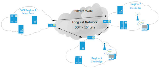
Figure 1.
Cloud Data Sharing Use Case over Heterogeneous Long Fat Networks (HLFNs).
In addition to transferring information between servers from different server farms, it also exchanges large amounts of stored data between cloud servers and endpoints. These end nodes can be connected through a wired or a short-range wireless connection. Given the short-range wireless connection and the endpoints’ data transfer profile (large amount of stored data), mobility during the transfer is not expected, nor are there a high number of intermediate nodes due to the network topology.
On the one hand, the AATP protocol provides a high-performance data transmission and quick recovery in case of a loss episode. However, on the other hand, its performance is affected over lossy wireless networks because the protocol does not recognize random channel losses. Its lower operation requires an adaptation to deal with the complexity of the Cloud Data Sharing Use Case over Heterogenous Long Fat Networks. In addition, given the possibility of having different AATP flows connected to the same end-device or server, the unfriendly behavior of the AATP is required to be modified to achieve intra-protocol fairness. To overcome these drawbacks, it is necessary to propose solutions for the paradigm of HLFNs.
For these reasons, a review of the State-of-the-Art of the most outstanding transport protocols designed for wireless networks is detailed. Specifically, it focuses on the operation of these protocols, the reference metrics, and their mechanisms to deal with the inconveniences of the radio media. Finally, different fairness indices are considered to define a mechanism for the fair distribution of the bandwidth among the distinct flows connected to an endpoint.
3. Related Work. Metrics Selection Process
The main cause of losses in wired networks is the congestion of one of the intermediate devices [17]. To correct this situation, the endpoint reduces its sending rate to reduce network saturation. However, when a loss occurs in a wireless network, it can be caused by a change in channel conditions (fading, interferences) [2]. In HLFNs [3], these drawbacks are more critical. In this section, distinct metrics are analyzed and are selected to be included in the protocol for the decision-making process. Moreover, in the case of wireless shared media, the fair distribution of the network resources, from the nodes’ point of view is more difficult to control [18] because of its channel characteristics.
3.1. Wireless Oriented Transport Protocols. Wireless Channel-Loss Metric
Relating the actions taken by a protocol to network statistics is an interesting approach for the decision-making process on network events. The Performance-oriented Congestion Control (PCC) [19], defined by Mo Dong et al., makes controlled decisions based on empirical evidence, pairing actions with directly observed performance results.
In order to evaluate the metrics and mechanisms for wireless loss-tolerant transmissions, diverse transport protocols solutions and their congestion controls have been studied. Cheng Peng Fu and S.C Liew proposed TCP Veno [20], based on TCP Reno and TCP Vegas [21,22]. This protocol calculates the Round-Trip Time (RTT) periodically, recording the minimum RTT of the communication, known as Base RTT or Best RTT, and the last RTT, known as Actual RTT. TCP Veno bases its loss episode decision on the comparison of these two RTT values, also taking into account the Congestion Window and the bottleneck of the connection.
A multipath feature is introduced in mVeno [23] by Pingping Dong et al. to improve the performance of the protocol by using the information from the subflows that belong to a TCP connection. The objective is to adaptively adjust the transmission rate of each subflow and acting over the congestion window, decreasing one-fifth of it, in the case of a packet loss event.
With reference to the TCP Reno mechanism, Taha Saedi and Hosam El-Ocla proposed the Congestion Control Enhancement for Random Loss (CERL) [24,25] and its revisited version, CERL+ [26], to improve the performance over wireless networks. CERL+ proposes a modification of TCP Reno at the sender-side by using a dynamic threshold of the RTT. With the average RTT, the protocol calculates the length of the bottleneck’s queue to evaluate the congestion status and distinguish a random loss. The main drawback pointed out by its authors is the requirement of precise time synchronization between the sender and receiver.
Saverio Mascolo et al. built TCP Westwood [27] and its evolution TCP Westwood+ [28]. This protocol differentiates the loss episodes by defining a coarse timeout for congestion loss and by setting the reception of three duplicated ACKs (DUPACKs) as the indicator of channel loss during the bandwidth estimation process. An upgraded slow-start for Westwood was proposed to improve its performance [29].
The Dynamic TCP (D-TCP) [30], proposed by Madhan Raj Kanagarathinam et al., extracts the end-to-end performance statistics (traffic intensity, link capacity, packet sending rate) of the connection to calculate the available bandwidth of the network. In case of abrupt changes or lossy conditions, D-TCP can adapt its operation by fixing a dynamic congestion window factor N. By adaptatively modifying the CWND, based on the factor N, the protocol avoids losing performance during a spurious packet loss event.
Venkat Arun and Hari Balakrishnan defined Copa [31], a practical delay-based protocol. Even if it is not focused on wireless environments, this protocol proposes a mechanism by fixing a target rate. This target rate provides a reference for high throughput and low delay. By relating the minRTT (the minimum RTT calculated in a long period of time) to the standing RTT (the smallest RTT over a recent-time window), the protocol adjusts its congestion window in the direction of the reference target rate. Moreover, Copa has a competitive mode to compete with buffer-filling protocols, based on the information extracted from the last 5 RTTs to check if the queue has been emptied.
Yasir Zaki et al. presented Verus [32], which is a protocol that focuses on the delay over high variable cellular channels. This protocol establishes a delay profile, which reflects the relationship between the congestion window and the delay variations, which is determined through the RTT, over short epochs. Verus uses this relationship to increment or decrement the congestion window based on short-term packet delay variations.
Neal Cardwell et al. presented TCP BBR [33], one of the most high-performance TCP protocols, which manages the maximum BW with the minimum RTT. Given the inefficiency of BBR in exploiting the Wi-Fi bandwidth, a modification is proposed by Carlos Augusto Grazia et al., which is called BBRp [34]. This inefficiency lies in the impossibility of performing frame aggregation because TCP BBR implements its own solution of the TCP pacing algorithm. Tuning the BBR pacing speed allows the congestion control to correctly aggregate packets at the wireless bottleneck with almost optimal TCP throughput.
To fulfill the needs of high-bandwidth requirements of last multimedia technologies (4K, VR/AR) over wireless connections, Li Tong et al. presented the protocol TCP-TACK [35]. This protocol bases its operation on two types of ACKs, the Instant ACK (IACK) and the Tamed ACK (TACK). The first one, IACK, is meant to get rapid feedback, which provides information about instant events (loss, state update.). The second one, TACK, is more focused on statistics (losses, available bandwidth, receipts, etc.). In this way, the number of ACKs sent to the network is reduced by over 90%, decreasing the overhead control and leading to an improvement of the goodput around 28%. Furthermore, TCP-TACK proposes an advanced way of calculating the minimum RTT using the smooth One-Way Delay (OWD) using relative values, reducing the information sent to the network without affecting the performance.
E. H. K. Wu and Mei-Zhen Chen designed Jitter TCP (JTCP) [36], which is based on the concept of the Jitter Ratio. Considering the sending time and receiving time of the packets, the Jitter ratio relates to the effect of the queued packets at the bottleneck the delay introduced between packets at the destination. The Jitter Ratio is compared to the Queue Decision maker (k/w), which is defined as the number of queued packets (k) considered as a congestion trace after all the packets of a congestion window (w) have been sent. If the Jitter Ratio is greater than the Queue Decision maker, this implies that the loss episode is due to congestion. If it is lower than Queue Decision maker, the loss episode is caused by the channel. JTCP defines one queued packet (k = 1) as a trace of congestion because TCP control flow increases its throughput by one packet per iteration. The operation with k > 1, more than one packet, is not analyzed or evaluated.
Jyh-Ming Chen et al. proposed an enhancement for the Stream Control Transmission Protocol called Jitter Stream Control Transmission Protocol (JSCTP) [37]. The JSCTP keeps the semantics and operation from the SCTP, adding a calculus of the aforementioned Jitter Ratio proposed in the JTCP for the loss episode decision. To filter the case Jr = 0, the Jitter Ratio is smoothed.
The TCP Jersey, presented by Kai Xu et al., [38], and its evolution, TCP New Jersey, estimate the total bandwidth of the connection and, with the information provided by the timestamps of the ACK received, decide if the loss episode is due to congestion or the channel. These protocols include the flag Explicit Congestion Notification (ECN), which uses the information provided by the intermediate routers on their queue status to make the final decision. Different protocols rely on these feedback mechanisms from the network devices, which are out of the scope of this paper because these functionalities are not usually enabled on the intermediate routers. V. B. Reddy and A. K. Sarje proposed TCP-Casablanca [39] for these types of mechanisms to decide the type of losses by considering the flag set by the intermediate routers. These routers have a biased queue management to identify the retransmitted packets.
New data-driven designed protocols are out of the scope of this work, as is the protocol algorithm Indigo [40] from Francis Y. Yan et al., which applies machine learning, given the requirements needed to train the protocol and the amount of data needed for this process. Indigo uses a machine-learned congestion control scheme from the data gathered from Pantheon [41], which is a community evaluation platform for academic research on congestion control from Stanford University. Indigo observes the network state each time an ACK is received, adjusting its congestion window every 10 ms while updating its internal state.
After analyzing the most outstanding transport protocols for wireless loss-tolerant transmissions, Table 1 depicts the wireless loss decision metrics used by each analyzed protocol. The analyzed protocols propose the combination of different metrics related to the Round-Trip Time (or Delay-based), Jitter, information from different flows and the queue, buffer, or congestion, and status of the network or the intermediate routers to find out the cause of a loss over a wired-wireless network.

Table 1.
Wireless loss decision elements from the wireless loss-tolerant transport protocols.
The metrics related to the information provided by the network nodes (ECN) are discarded from the metric decision due to the fact that this information from the network may not be accessible. Data-driven machine learning techniques are also discarded, given the requirements requested to train the protocol and the amount of data needed for this process.
In addition, delay-based solutions are not considered because of the buffer-fill profile of the AATP protocol. The use of the Round-Trip Time is also discarded, given the high delay of HLFNs, the ACK actions, and the synchronization requirement.
Finally, given the packet burst operation of the AATP, the time difference among the packets received provides information about the status of the bottleneck, which can be directly related to the jitter. The jitter provides information about the intermediate nodes packet queue. None of the Jitter Ratio-based protocols consider the possibility of adding more than one packet per iteration.
In this paper, in order to overcome the aforementioned drawbacks, the Enhanced-AATP proposes a Loss Threshold Decision maker (LTD) mechanism. The LTD is compared to the Jitter Ratio, considering the possibility of adding more than one packet per iteration. The Jitter Ratio increments its value as the saturation of the intermediate nodes increases, providing information about a possible congestion episode.
3.2. Fairness Indices. Intra Fairness Multi-Flow Metric
The concept of fairness is analyzed, and distinct indices are evaluated by the AATP enhancement to obtain a controlled fair share of the network’s resources by different flows connected to the same node.
The fairness concept refers to how fair the treatment is between the different nodes that are sharing a specific resource. In the environment of networks and the Internet [42], the concept refers to the fairness in the distribution of the throughput that can reach each of the flows that share a point-to-point connection. Modern protocols have required the introduction of a fairness system as in the case of BRR [43].
Usually, most of the networks are IP best-effort, in which there is no point-to-point control of the resources and in which losses can occur due to congestion or channel failure, directly affecting the quality of the connection. However, to achieve proper fairness, the different flows must be treated fairly, equally, and impartially. Another possible approach is to give preferential treatment to the flows that require more resources at the request of the system or the user [44].
Shi, H. established in [45] a way to measure the fairness of a system (or of the individuals in a system), where various types of indices are used to quantify this notion of equality and fair treatment. These indices quantify fairness based on certain metrics (throughput is one of the most used) that are evaluated by each of the flows. In this way, the initial assumption is made that there is a type of resource whose total is Cx, which has to be distributed among n individuals. In this way, the location X = {x1, x2, …, xn} is obtained, where xi is the amount of the resource provided to element i. Thus, must be satisfied, where Cx is the total amount of the resource that can be provided. In this way, a function f(X) must be defined to give a quantitative value of the system’s fairness. Said function f(X) should meet the following requirements:
- R1: f(X) should be continuous in .
- R2: f(X) should be independent of n.
- R3: The range of values of f(X) should be mappable to [0, 1].
- R4: f(X) should be scalable to multi-resource cases.
- R5: f(X) should be easy to implement.
- R6: f(X) should be sensitive enough to the variation of X.
To compare the different fairness indices, other significant aspects are defined to consider:
- Definition: The index must meet the definition of fairness.
- Measurable: Fairness must be measurable quantitatively.
- Unfairness: The method should make it possible to detect which individuals are not treated fairly.
- Priorities/Weights: The method must allow weight assignation to give priority to some individuals over others.
- Control: Fairness control and possible index requirements for information on system data are also considered.
- Function f(X) requirements: The definition of the function f(X) meets the six aforementioned requirements (continuous, independent, mappable, scalable, implementable, and sensitive).
The indices analyzed are Jain’s Fairness Index, Entropy Fairness, Max-Min Fairness, Proportional Fairness, Tian Lan’s Index, and Envy-Based Fairness, which are compared in Table 2.
Table 2.
Fairness indices comparison [45].
The index that meets the most requirements is Jain’s Fairness Index. The fairness calculation, according to Jain’s Fairness Index (JFI) is calculated from the J function:
where is the amount of the resource that is given to flow for each of the flows that make up the system. The values that the function can take are in the range [0, 1]. A value of J = 1 indicates that there is total fairness in the whole system, while a value of J = 0 indicates that the system is totally unfair. From this function, samples can be taken periodically to obtain a discrete function that depends on time and is able to analyze the trend of the system, obtaining the following equation:
Although this method helps to give a general idea of the fairness of the system, not giving weights to the flows does not help us to find at which points the fairness is not fulfilled [46]. For example, it has been found that a difference between J = 0.9 and J = 0.8 has a different effect on the behavior of the different flows compared to a difference between J = 0.6 and J = 0.5; although in both cases, the difference is 0.1 [42]. Furthermore, the JFI assumes that all flows are equally capable of consuming the resources for which they are competing, although in reality, this may not be the case.
In this paper, a modification of the JFI is proposed for a Weighted Fairness (WF) calculation in the Enhanced-AATP, which considers the possibility of prioritizing flows.
The modifications proposed in this section for the improvement of the AATP over heterogeneous networks directly affect the base operation of the protocol, which is reviewed in the following section.
4. AATP Review
In this section, the Aggressive and Adaptative Transport Protocol (AATP) [14] is reviewed to provide a recap of the protocol operation and its mechanisms before introducing the improvements.
A specific Cloud company set high-level data exchange requirements between their servers’ farms deployed in Storage Area Networks (SANs) from remote branches in different regions. The AATP protocol was designed to overcome the limitations of transport protocols over Long Fat Networks [3]. In order to achieve an optimal communication performance, the protocol was designed with the following characteristics:
- Connection-oriented: The objective is to avoid TCP’s synchronicity and its rigid overhead. For this reason, the AATP proposes an in-band control of the packets over IP. Compared to TCP and UDP, the use of the Selective ACK and its control of the gaps (lost packets) provides an asynchronized controlled data exchange and lost packets are requested.
- Efficient: The Bandwidth Estimation process calculates the maximum bandwidth capacity of the communication, reaching the upper limit of the link during data transfer (>95%).
- Adaptable: The protocol reacts to a loss episode, reducing its throughput. After detecting the end of the loss episode, the protocol increases its throughput directly to reach 80% of the calculated link capacity. After that, the protocol increases it gradually to avoid causing congestion.
- Friendly aggressive: The protocol is focused on the maximum use of the capacity of the link (>80%), and the residual bandwidth is left for the other protocols (<20%).
For the initial BW estimation, 10 bursts are sent following the technique of packet trains (groups of two to 20 packets). The Source sends the packets of each block (burst) consecutively. After that, the Destination sends a confirmation message on receipt of the last packet of the block.
For each burst, the reception times of the first and last packets are recorded, and the difference () is calculated. Once information on the size of the packets (b) in bits and the packets that have been received (N) is obtained, the bandwidth of the link () for that burst can be calculated
Once the Destination has received the ten bursts, ten values of the estimated bandwidth are obtained, using the arithmetic mean of these values as the definitive one .
At the beginning of the data transfer, the initial transmission speed (Sending Rate—SR) is set, fixing it at a percentage of the maximum bandwidth one . It depends on the desired aggressiveness.
The data are sent by bursts, which are separated by a period () determined by the RTT or the minimum temporal resolution that can be offered by the operating system (OS) and the hardware (HW) on which the process operates. This time will be calculated in milliseconds or microseconds.
Once we know the speed at which the packets are initially sent (in packets per second) and have determined the separation between bursts, the number of packets sent in each burst is
The receiver decreases or increases the SR value depending on whether or not any packets have been lost in the last burst, which is calculated by
where is the size of the packet in bytes. When losses are detected, the higher the use of the link, the greater the reduction in the SR.
The value of the , packet increment (packets), follows the philosophy of UDT [47] and uses a DAIMD (AIMD with decreasing increases) logarithmic function. This function is based on the usage of the estimated link capacity. On the one hand, when the SR value (converted to bps) is far from the estimated link capacity (meaning low efficiency), the increase of packets per each burst is high to achieve greater throughputs fast. On the other hand, as the link utilization keeps growing (meaning higher efficiency), and the increase of packets to be sent per each burst gets smaller. This strategy has been proved to be stable and efficient [48]. The value is determined by
causing a logarithmic growth of the SR. In relative terms of the link’s capacity usage, the growth of the SR always experiences the same behavior (in a zero-loss scenario) thanks to the logarithmic function. Psize—in bytes—and 8 are conversion factors to get the SR value in bps. When the use of the link is low, the increase in the speed of transmission is greater, and vice versa.
The value M is a magnitude modifier that reduces the orders of magnitude of the power function. It is necessary to reduce these orders of magnitude because if they were not reduced, the final SR value would be enormous and vastly surpass the estimated bandwidth. Thus, the M value aims to adapt the number of packets to be increased per burst depending on the estimated bandwidth utilization. It is a design value that can be fine-tuned, but it should be large enough to moderate the results of Equation (8) and get reasonable SR values. As an example, the logarithmic function of UDT is always reduced by nine orders of magnitude. We do not use the same value because the UDT formula calculates packets per second, while the AATP formula calculates packets per burst. In our case, after several iterations of simulations, we found that a value of 7 was big enough to achieve high increases in SR values in situations where the estimated link utilization was below the 80% of its estimated value. When the link’s utilization is equal to or greater than 80%, the order of magnitude to be reduced must decrease linearly as efficiency increases. This way, the M value helps to shape the SR logarithmic growth more aggressively at low-performance episodes and more steadily at high-performance ones. The calculation of M is based on the following formula
being more aggressive when efficiency is worse than 80% to achieve high-throughput levels without saturating the connection. Figure 2 shows the growth of the SR value (in Mbps) over a 1 Gbps link in an ideal situation without losses and an estimated bandwidth of 1 Gbps.
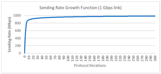
Figure 2.
Sending Rate Growth Function over 1 Gbps link in an ideal situation without losses. Sending Rate (Blue).
Although the objectives of the protocol are clear (efficient, adaptative, and friendly aggressive) and accomplished, the AATP presents two main drawbacks if the protocol is used over Heterogeneous Long Fat Networks:
- Lossy episodes are all assumed as a congestion episode, without differentiating channel losses from congestion losses in heterogeneous scenarios. The efficiency of the protocol decreases because the Sending Rate is reduced in a channel loss episode and the time to recover the high-performance throughput directly affects its capability.
- There is no fair flow prioritization to fairly share the node network resources efficiently without causing losses and instabilities because there is no control between both flows.
5. Enhanced-AATP
The Enhanced-AATP is an improvement of the AATP protocol, which proposes solutions to solve the aforementioned drawbacks of the protocol over Heterogeneous Long Fat Networks. As stated before, the protocol AATP is efficient and adaptable in networks with high bandwidth and high delays (LFNs), but when it is used in heterogeneous networks, it is not able to differentiate distinct types of losses. Moreover, because of its aggressiveness, the protocol is unfair with other AATP flows.
The objective of the Enhanced-AATP is to adapt the protocol to achieve high performance over HLFNs and fairly sharing the network resources with the other flows that coexist in the same node. In this section, the operation of the Enhanced-AATP, together with its two new functionalities, is presented:
- Loss differentiation mechanism. The protocol identifies if the loss episode is due to congestion or a channel failure through a Loss Threshold Decision maker (LTD), which bases its operation on a Jitter Ratio comparison.
- Prioritized fair share of node network resources. This mechanism manages the Enhanced-AATP flows exchanged information with one node to achieve the deserved speed for each of them regarding their prioritization.
These imply a modification of the data exchange process of the protocol and its mechanisms, introducing the Loss Threshold Decision maker functionality and the Weighted Fairness mechanism.
5.1. Data Exchange Process
The Enhanced-AATP data exchange process is detailed to show the data process and how the metrics are measured. Figure 3 shows the protocol operation and how the information is sent and processed.
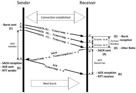
Figure 3.
Enhanced-AATP data exchange process.
Following the numbers (1) to (6) of Figure 3, the data exchange process of the Enhanced-AATP is explained:
- (1)
- After the connection is established and the Estimated Bandwidth is measured, the Sending Rate is decided (% of the Estimated Bandwidth). The Sender sends a burst to the Receiver, recording the timestamp of each packet sent.
- (2)
- The Receiver registers the time reception of each packet.
- (3)
- After receiving the last packet of the burst, the Jitter Ratio is calculated
- (4)
- At this point, the Receiver sends a SACK message confirming the reception of the burst and the Jitter Ratio.
- (5)
- The Sender registers the Jitter Ratio and the reception time to calculate its RTT. At the same time, he replies to the Receiver with an ACK message to confirm that it will adjust the to the new SR and (RTT).
- (6)
- The Selective ACK is acknowledged. The Receiver records the reception time to calculate its RTT. This information is taken for network statistics in case a transfer is initiated in the other way. The next burst is sent.
5.2. Loss Differentiation Mechanism—Loss Threshold Decision Maker (LTD)
After detailing the data exchange process, the operation of the loss differentiation mechanism is defined. The Enhanced-AATP introduces the Loss Threshold Decision maker as a way to distinguish the cause of the losses produced during the communication. At this point, given the HLFNs characteristics, it is necessary to obtain a reference metric that is not affected by the high delay of this type of networks and that is asynchronous to the endpoints. The metric used for the loss decision is the smoothed Jitter Ratio (), which is defined in (11).
Since the Jitter Ratio is the reference metric to check the origin of a loss episode, it is necessary to determine the threshold. As soon as a queue is formed in the bottleneck device due to a saturation episode, it is detected by the Destination node through the value of the Jr, thus preventing an overflow in the buffer and packet discard. The Jr value calculation is increased because the time between packet arrivals at the Destination is greater as a result of the formation of queues at the bottleneck. Following the network’s operation process, if the bottleneck device is fully saturated after a new burst is sent and it starts to drop packets; these additional packets will provoke an overflow in the intermediate device, causing a congestion loss episode.
In the case of the aforementioned JTCP and JSCTP, the Jr is fixed to one packet over the congestion window because the basis is TCP. In the case of the Enhanced-AATP, this design value is different because of the way the protocol operates as it can increase its Sending Rate by more than one packet per burst. The Loss Threshold Decision maker () is defined by the number of increased packets in the burst over the total number of packets of the burst.
The reason for this LTD proposal is because in each iteration without losses, a number of new packets () are included in the burst (). If a congestion loss occurs, it means that the buffer of the bottleneck is overflowing as a result of the new packets included in the last burst.
The defined is compared to the . This comparison will differentiate when a loss episode is because of a misfunction of the channel or the congestion in the network or when the rises as the intermediate router generates a packet queue caused by saturation. When the remains stable because there are no packet queues in the intermediate router (no saturation), the channel has most likely suffered a failure (fading, interference).
Depending on the situation detected, the Enhanced-AATP reacts differently to the loss episode. Four different states are defined, which are detailed in Table 3 and described below.
Table 3.
Enhanced-AATP operation states.
(S0) No loss episode and ≤ . The sending rate is increased, depending on the efficiency registered.
(S1) No loss episode and > . On receipt of this information, the sending rate is moderately increased (M = 9), as if the sending rate was reaching the limit.
(S2) Loss episode and ≤ , meaning a channel loss episode. The sending rate is kept at the same speed. As soon as the communication starts working again without losses, the lost packets are requested again.
(S3) Loss episode and > , meaning a congestion loss episode. The sending rate is reduced. As soon as the communication starts working again without losses, the sending rate is increased.
5.3. Fairness Mechanism
In order to procure a fair share of network resources from the destination, the fairness mechanism is presented. The adopted Fairness index is the Jain Fairness Index (JFI). The only requirement that is not fulfilled by the JFI is the weighted priorities of the flows. As a result of this reason, the JFI is modified to provide it to the Enhanced-AATP. The metrics to consider in the Weighted Fairness calculation are:
- Internal factors.
- ○
- Number of Flows ().
- ○
- Priority of each flow (). Its value can be any integer between 1 and 8 (both inclusive). This way, the priority value can be mapped to other QoS classifications (IP Precedence and 802.1p).
- External factors.
- ○
- Estimated Bandwidth () [bps].
- ○
- Network status (characteristics, statistics, and behavior).
- Real throughput of a flow () [bps]. Where is the packets sent per second [packets/second], is the packet size [Bytes] and 8 to convert bytes to bits.
- Allocated throughput for a flow () [bps]. This formula provides the allocated throughput assigned to the flow regarding its priority (), the sum of all priorities (), and the available bandwidth ().
- Efficiency () of a flow . It determines the percentage of the throughput achieved by the flow regarding the allocated speed.
With these defined metrics, the Weighted Fairness () can be calculated as follows, being the JFI the base:
If the value is 1, there is a fair share of the resources. Otherwise, if the value is 0, the system is not working properly. In contrast to the JFI, this way of calculating the fairness considers the real throughput of each flow, the priority provided to these flows, and their allocated throughput decided by the system, considering the estimated bandwidth.
The protocol is able to modify its operations and flow behavior because of the and its performance.
The main modification is the number of packets to be increased or reduced at the time of calculating the Sending Rate (no lossy episode; S0 and S1) to adapt the flow to the deserved speed. It is done with the Adapter ().
where is the allocated throughput of the flow, is the real throughput of the flow, and is the Transcendence factor. A logarithmic function is used to shape three different behaviors. Firstly, if the current throughput of the flow is below its maximum, packets per burst should be increased. This is achieved because, in this case, so . Secondly, if the current throughput of the flow is above its maximum, the number of packets per burst should decrease to achieve fairness. This is also possible because when , . Thirdly, if the throughput of the flow is equal to its maximum, it behaves fairly, so packets per burst should not be increased or decreased. This behavior is also satisfied because when , . A simple quotient could not be used, because the result would always be positive, so packets per burst would always increase. A subtraction would satisfy the three behaviors, but it would depend on the absolute values of throughput instead of relative values of utilization, which would result in excessive values of . For this reason, the use of a logarithmic function was chosen.
Despite that, the values obtained in the logarithmic function might be too small when compared to the values of , making the fairness mechanism insignificant when compared to the congestion control. Thus, the Transcendence factor A is needed to give relevant importance to the fairness mechanism, with a comparable influence on congestion control. The higher the value of , which should be related to the , the higher the value of . This implies a more aggressive increase in the Sending Rate or a decrease when is negative and , reducing the convergence time to balance the weighted distribution of resources. This fact can affect the stability of the system due to sudden changes.
The value of A is a design parameter that can be adjusted. The greater the value is, the greater the importance of the fairness mechanism over the congestion control. In our case, the factor is defined by
thus, relating it to the , the number of flows (N), and the estimated bandwidth (BW). The A factor is directly proportional to the estimated bandwidth because more packets can be sent per burst at a higher bandwidth. Moreover, it is inversely proportional to the number of flows because the packets to be increased or decreased per burst should be distributed among all flows. It is related to the too, in a way that when the system is behaving more fairly ( value close to 1), the fairness mechanism has less relevance, while in unfair scenarios ( value not close to 1), it has a greater impact.
and are design parameters that help to fine-tune the degree of aggressiveness of the Transcendence factor (A). and are standard values to relate the A factor directly to BW and inversely to N. In our case, after several iterations of simulations, and are the used values in our tests that provide a suitable balance between the and parameters as well as faster convergence in fairness.
Instability occurs when the designation of a Sending Rate is higher or lower than the ideal one, thus requiring a new iteration to achieve the ideal speed of each flow. The degree of instability is related to the suddenness of the change in the Sending Rate. If the value of A is not high, the convergence time is longer, since slight modifications are made on the SR. However, the probability of instability in the system is reduced since there are no sudden changes in the Sending Rate, causing a fine-tuning.
Once the Weighted Fairness mechanism is introduced, the congestion control needs to slightly modify Equations (7)–(9) as each flow aims to reach its allocated throughput () and not the total Bandwidth of the link (BW).
6. Enhanced-AATP Evaluation and Performance Simulations
In this section, the Enhanced-AATP protocol is simulated and evaluated by the Steelcentral Riverbed Modeler [15]. The new functionalities are tested through different experiments to validate its operation and performance.
The Riverbed Modeler testbed scenario is detailed in Figure 4, which simulates a Long Fat Network with different possible configurations. In most scenarios, the bottleneck has a bandwidth of 148.608 Mbps (OC-3 link), and the maximum bottleneck capacity tested in the simulations is 1 Gbps. The packet size is fixed at the MTU of the media technology, and the propagation delay is the speed of light in the backbone. The minimum base RTT of the WAN link is 20 ms, so the Bandwidth-Delay Product (BDP) is always greater than 12,500 bytes (105 bits)).
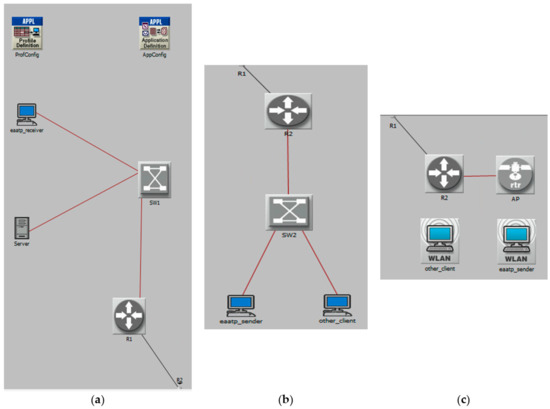
Figure 4.
Testbed scenario over a Steelcentral Riverbed Modeler. (a) Storage Area Network (SAN) side and Client edge with (b) wired endpoints or (c) short-range wireless endpoints.
Although the connection between both routers consists of a single link, distinct random generation seeds are defined in the simulator to introduce variability in the network. The environment is configured to simulate the characteristics and behavior of a Heterogeneous Long Fat backbone, depending on the requirements of the experiment (different speeds, random losses, delay depending on the distance).
The Testbed is composed of a Storage Area Network (SAN) region and a Client edge. In the SAN side, there are servers from the server farm connected through a wire to the gateway that gives access to the WAN (a), and in the Client edge, two nodes are deployed. One is an Enhanced-AATP node (eaatp_sender), and the other node (other_client) is introduced to provoke different scenarios (different types of cross-traffic, interference generation). The cross-traffic can be a TCP flow with a Variable Bit Rate (VBR) or a UDP flow with a Constant Bit Rate (CBR). These nodes from the Client side can be connected through a wire (b) or a short-range wireless (WiFi—802.11n) (c), while the speed and Ethernet technology can be varied depending on the experiment and the objective to be achieved.
The experiments and their objectives are listed below:
- Maximum performance in wireless. The objective is to verify the efficiency of the protocol over wireless. This experiment exhibits the maximum performance of the Enhanced-AATP protocol over different wireless speed connections without other flows or random losses. The scenario is Figure 4a connected to Figure 4c.
- Random loss episode detection. The objective of this experiment is to demonstrate the channel loss identification and the proper operation of the protocol in this specific case (Table 3—(S2) Channel loss). This experiment shows that the protocol identifies the different random loss episodes occurred and reacts by keeping its Throughput and Sending Rate. The scenario is Figure 4a connected to Figure 4c.
- Loss Threshold Decision maker (). The objective is to prove the correct differentiation of distinct types of losses. Moreover, the optimal value is evaluated. In this experiment, distinct cross-traffic (load) and different random losses are introduced. The operation of the protocol and the performance are presented, differentiating congestion losses and channel errors that occurred during the communication. The scenario is Figure 4a connected to Figure 4c.
- Enhanced-AATP performance comparison. The objective of this last experiment is to compare the Enhanced-AATP performance (throughput, one-way delay and losses) with the modern protocols analyzed. A specific scenario is deployed.
The outcomes shown are the mean results of different executions (around 1000 in total, 30 simulations run per test, except the value test, which implied 650 simulations), assuring a maximum error deviation of ±1.5% with a confidence interval of 99%.
6.1. Maximum Performance in Wireless Connections
The performance of the Enhanced-AATP over heterogeneous networks without cross-traffic nor random losses is studied in this set of tests, where the bottleneck is the wireless section at different link speeds. The scenario is Figure 4a connected to Figure 4c.
Figure 5 exhibits the Enhanced-AATP performance, showing the average (orange) and the median with second and third quartiles (blue) of the Throughput and Sending Rate over different link speed scenarios. The selected wireless link speeds are 6.5 Mbps (a), 30 Mbps (b), 120 Mbps (c), 300 Mbps (d), and 600 Mbps (e). The duration of the transfer is 60 s.

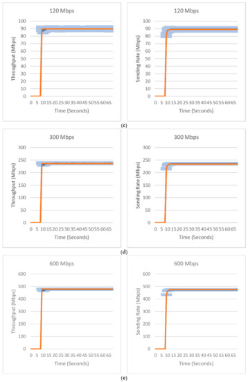
Figure 5.
Enhanced-AATP performance over different wireless networks without cross-traffic and random losses. Average Throughput and Sending Rate (orange), the median with quartiles (blue). (a) 6.5 Mbps link capacity, (b) 30 Mbps link capacity, (c) 120 Mbps link capacity, (d) 300 Mbps link capacity, and (e) 600 Mbps link capacity. No losses occurred.
From Figure 5, the summary in Mbps is extracted in Table 4 to compare them with the maximum capacity of the link in each bottleneck situation. Given the limitation of the CSMA/CA, as Apoorva Jindal and Konstantinos Psounis presented in [49], in any realistic topology with geometric constraints because of the physical layer, the CSMA-CA is never lower than 30% of the optimal used to access the media in wireless. In the case of Enhanced-AATP, the maximum bandwidth used in these links goes from 72% to 80%, keeping to the aforementioned limitation and working with higher efficiency over high-bandwidth links due to the design of the protocol for Long Fat Networks.
Table 4.
Enhanced-AATP performance over different wireless networks.
6.2. Random Loss Episode Detection
In order to check the Enhanced-AATP mechanism to detect random losses, distinct tests are run simulating loss episodes of different periods of time. In this case, the bottleneck is placed on the wired section (OC-3 (148.608 Mbps)) to avoid the effect of the CSMA/CA shown in the previous set of tests, without affecting the loss detection mechanism and its performance. The scenario is Figure 4a connected to Figure 4c.
In order to depict the Enhanced-AATP’s random loss identification and behavior using the LTD mechanism, its operation is shown together with other TCP protocol’s behavior without the LTD maker (TCP Cubic). The main goal of this comparison is to show how the Enhanced-AATP identifies the channel losses occurred (fadings with 100% of losses), while TCP introduces load to the network and also reacts to the fading, reducing its throughput as it was caused due to a congestion in the network. It also affects the transmission time.
Figure 6 illustrates the Throughput obtained by the Enhanced-AATP, average (orange), and the median with second and third quartiles (blue) and TCP Cubic (green), and the time required to send 1 GB in different channel loss situations. First, a case without losses is shown (a) to be the reference in time spent and Throughput performances. After that, the random loss episodes experiments are 10 random losses of 0.5 s (b), 10 random losses of 1 s (c), and 5 random losses of 2 s (d).
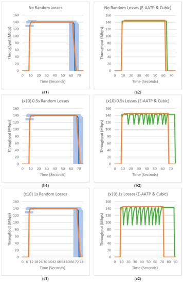
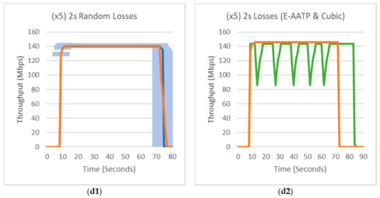
Figure 6.
Enhanced-AATP performance with random losses. Enhanced-AATP Throughput (orange), its median with quartiles (blue) and TCP Cubic Throughput (green). (a1) No random loss—Averaged Enhanced-AATP, (a2) No random loss—Enhanced-AATP and TCP Cubic, (b1) 10 random loss episodes of 0.5 s—Averaged Enhanced-AATP, (b2) 10 random loss episodes of 0.5 s—Enhanced-AATP and TCP-Cubic, (c1) 10 random loss episodes of 1 s—Averaged Enhanced-AATP, (c2) 10 random loss episodes of 1 s—Enhanced-AATP and TCP-Cubic, (d1) 5 random loss episodes of 2 s—Averaged Enhanced-AATP and (d2) 5 random loss episodes of 2 s—Enhanced-AATP and TCP-Cubic.
Packet queues are not formed because no bottleneck saturation occurs, so the Jr value is not increased. When a channel loss episode occurs (100% of losses), through the comparison, the protocol identifies it and keeps the Throughput achieved before the losses, as shown in the graphs above. Figure 6 shows the behavior of the Enhanced-AATP protocol in different random loss situations.
- Figure 6a is the reference performance for the protocol because no losses occur. The Enhanced-AATP spends 54 s with a mean throughput of 145.36 Mbps. TCP Cubic spends 57 s with a mean throughput of 140.96 Mbps.
- In Figure 6b, 10 episodes of 0.5 s of random losses are introduced, being a total channel loss time of 5 s. In Figure 6(b1), the protocol keeps the throughput (145.38 Mbps) and spends approximately 5 more seconds than the reference. In Figure 6(b2), the Enhanced-AATP operation is shown together with the TCP protocol (TCP-Cubic), which modifies its throughput (135.03 Mbps) due to the losses, spending 11 s more.
- In Figure 6c, 10 episodes of 1 s of random losses are introduced, being a total channel loss time of 10 s. In Figure 6(c1), the protocol keeps the throughput (145.38 Mbps) and spends approximately 10 more seconds than the reference. In Figure 6(b2), the Enhanced-AATP operation is shown together with the TCP protocol (TCP-Cubic), which modifies its throughput (129.29 Mbps) due to the losses, spending 24 s more.
- In Figure 6d, 5 episodes of 2 s of random losses are introduced, being a total channel loss time of 10 s. In Figure 6(d1), the protocol keeps the throughput (145.35 Mbps) and spends approximately 10 more seconds than the reference. Figure 6(d2) shows the Enhanced-AATP operation together with the TCP protocol (TCP Cubic), which modifies its throughput (131.38 Mbps) due to the losses, spending 19 s more.
From Figure 6, the success detection rate for 100% channel losses (fading) is 1 because, compared with the TCP behavior shown, the Enhanced-AATP protocol keeps its throughput during a channel loss episode. If the detection was not successful (<1), the Enhanced-AATP’s throughput would experience decreasing episodes. Moreover, the performance of the Enhanced-AATP (Mbps) and the average transmission period (seconds) for each random loss episode test are extracted in Table 5. In addition, TCP Cubic’s performance (Mbps) and transmission period (seconds) are shown. Moreover, the time noted between parentheses in both Transmission period fields indicates the extra time dedicated by the protocol in reference to the case without random losses.
Table 5.
Enhanced-AATP and TCP Cubic performance with different random loss episodes.
In the case of the Enhanced-AATP, the average transmission period is equal to the average transmission period without loss episodes plus the channel losses’ duration, demonstrating the high performance (>97%) operation of the protocol during distinct channel loss situations (Figure 6b–d). The Enhanced-AATP depicted together with TCP Cubic provides a view about how the fadings affect the performance of TCP protocols (in (Figure 6(c2), more than a 10 s difference is noted between the Enhanced-AATP and TCP Cubic). Thanks to this experiment, the proper operation of the Loss Threshold Decision maker mechanism to identify the random losses of the channel is demonstrated.
6.3. Loss Threshold Decision Maker (LTD)
In this experiment, the comparison is tested to demonstrate the capacity of the Enhanced-AATP to differentiate the type of loss episode occurred. Distinct and varied loss episodes occur during the simulations run with best-effort TCP/UDP cross-traffic load is introduced. The control over the cross-traffic is limited because of simulator restrictions to manage the generic TCP (traffic trying to reach the maximum possible throughput, but with a Variable Bit Rate (VBR) traffic behavior profile due to its congestion control) and UDP flows (with a Constant Bit Rate (CBR) traffic behavior profile). The scenario is Figure 4a connected to Figure 4c.
Figure 7 shows the performance of the Enhanced-AATP with random losses episodes and cross-traffic sending a file of 1 GB, showing the average percentage of the link used by the Enhanced-AATP (blue) and the average percentage of the link used by the cross-traffic (gray). The experiments simulated are: no random losses with TCP VBR cross-traffic (a), no random losses with 20% UDP CBR cross-traffic (b), 1-s random loss (×5) with a TCP VBR cross-traffic flow (c), 1-s random loss (×5) with a 20% UDP CBR cross-traffic flow (d), 2-s random loss (×5) with a TCP VBR cross-traffic flow (e), and 2-s random loss (×5) with a 20% UDP CBR cross-traffic flow (f).
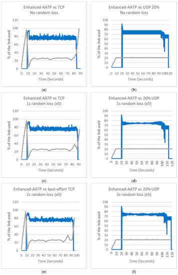
Figure 7.
Enhanced-AATP performance with TCP/UDP cross-traffic and random losses. Average percentage of the link used by the Enhanced-AATP (blue), Average percentage of the link used by the cross-traffic (gray). (a) No random loss episodes with TCP cross-traffic—11.65% of average losses, (b) No random loss episodes with 20% UDP cross-traffic—14.36% of average losses, (c) Five random loss episodes of 1 s with TCP cross-traffic—16.11% of average losses, (d) Five random loss episodes of 1 s with 20% UDP cross-traffic—18.48% of average losses, (e) Five random loss episodes of 2 s with TCP cross-traffic—20.14% of average losses, and (f) Five random loss episodes of 2 s with 20% UDP cross-traffic—22.29% of average losses.
Figure 7 depicts the result of the Enhanced-AATP in distinct cross-traffic loads and random losses situations. The aggressive behavior of the VBR and CBR flows in Riverbed act without considering the status of the network.
- Figure 7a show the result of the experiment when the Enhanced-AATP faces a TCP flow (trying to get the maximum bandwidth aggressively) without random losses. The TCP cross-traffic reaches around 24% of the residual bandwidth left by the Enhanced-AATP because of its aggressiveness, although TCP is trying to reach more. The improved protocol tries to take the maximum bandwidth possible, as the TCP flow tries to obtain the maximum bandwidth but in a less aggressive form, causing minor fluctuations of the Enhanced-AATP speed with a PLR of 11.65%. Considering the losses occurred because of the bandwidth conflict without random losses, in Figure 7c,e, the random losses are introduced (100%), and the PLR increases up to 16.11% (+4.46%, ≈5 s of 100% losses) in (c) and 20.14% (+8.49%, ≈10 s of 100% losses) in (e). The increment corresponds to the percentage of time while the random losses are occurring.
- Figure 7b shows the result of the experiment when the Enhanced-AATP faces a 20% UDP flow, which does not reduce its speed but directly affects the performance. In this case, the UDP does not modify its throughput, even when losses occur, generating moderate fluctuations of the Enhance-AATP throughput and more congestion losses, causing a PLR of 14.36%. Considering the losses occurred because of the bandwidth conflict without random losses, in Figure 7d,f, the random losses are introduced (100%) and the PLR increases up to 18.48% (+4.12%, ≈5 s of 100% losses) in (d) and 22.29% (+7.93%, ≈10 s of 100% losses) in (f). The increment corresponds to the percentage of time while the random losses are occurring.
From Figure 7, the success detection rate for 100% congestion losses is 1 because, during the coexistence between Enhanced-AATP with cross-traffic flows, the Enhanced-AATP tries to get the maximum bandwidth, reducing the throughput from the other flows. Due to this bandwidth’s conflict, a first level of convergence is reached (80%/20% distribution) and minor fluctuations occur due to the congestion produced by the two flows trying to obtain more bandwidth, which affects the network stability. In the case of a success detection rate lower than 1, the Enhanced-AATP’s throughput would be maintained, and more losses would occur due to a higher congestion of the network.
At this point, given the proper operation of the Enhanced-AATP protocol differentiating the type of losses, it is necessary to check if the Formula (14) is optimal to identify the type of loss occurred.
In Figure 8, the performance is evaluated by linking the transmission period (orange) and the lost packets (blue), modifying the original value from ×0.9 to ×1.1 in steps of 0.01. As shown in the graph, if the is compared with the 90% of the obtained value, the transmission period is increased while the total number of lost packets decreases. This means that some random losses are considered as congestion losses. On the other hand, if the is compared with the 110% of the obtained value, the transmission period is reduced. However, the lost packets are incremented, meaning that some congestion losses are treated as random losses, generating more saturation and more packets loss.
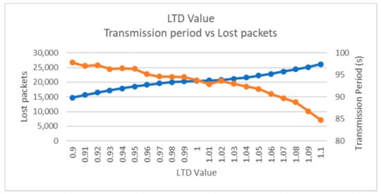
Figure 8.
LTD value evaluation. Transmission period (orange) and Lost packets (blue).
The objective is to find the optimal working point of the LTD for the consequent status of the network. Thanks to Figure 8, the optimal point in order to reduce the losses generated without increasing the transmission period is shown. The trade-off point between the transmission period and lost packets is the value obtained by relating directly the increased packets with the total burst. This result confirms the reasoning associated with the LTD design. After a congestion loss episode, the new packets included in the packet burst are the possible cause of the packet losses.
6.4. Fairness Mechanism
In this experiment, different priority levels are set to distinct Enhanced-AATP flows that share the destination endpoint. The scenario is Figure 4a connected to Figure 4b. The objective is to check the correct prioritized fair share of the network resources. The cases tested by priorities are: 1-1 (equal priority), 1-8 (maximum priority), and 2-4-6 (three flows).
Figure 9 presents the results of the different cases.
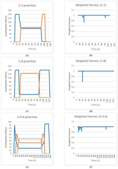
Figure 9.
Fairness mechanism with priorities. Case 1-1: Sending Rate of Flow 1 (blue) and Flow 2 (orange) (a) and its Weighted Fairness 1-1 (blue) (b). Case 1-8: Sending Rate of Flow 1 (blue) and Flow 2 (orange) (c) and its Weighted Fairness 1-8 (blue) (d). Case 2-4-6: Sending Rate of Flow 1 (blue), Flow 2 (orange) and Flow 3 (gray) (e) and its Weighted Fairness 2-4-6 (blue) (f).
- The first case, graphs Figure 9a,b, proposes two flows with the same priority (1-1). The flows share the bandwidth (Flow 1 (blue) and Flow 2 (orange), around 50% use each), and the fluctuates only during the introduction of the second flow and at the end of the transmission, keeping the value of 1, which means a fair share of the resources.
- The second case, graphs Figure 9c,d, aims to have two flows with a maximum difference priority (1-8). The flows share the bandwidth (Flow 1 (blue—11%) and Flow 2 (orange—89%)), and the is kept at 1, considering the prioritization established in its calculation.
- The last case, graphs Figure 9e,f, aim to launch three flows with different priorities (2-4-6). The flows share the bandwidth (Flow 1 (blue—16%), Flow 2 (orange—33%), and Flow 3 (gray—50%)), and its has different fluctuations at the beginning before the flows converge to its assigned speed, always converging to 1, thus generating the fair share of resources.
The fairness mechanism introduced regulates the flows without large fluctuations in the system thanks to the modification of the Sending Rate Formula (19)–(20). The weighted fairness measures successfully () the correct fair share of the resources considering the priorities of the flows.
6.5. Enhanced-AATP Performance Comparison
The objective of this last experiment is to compare the Enhanced-AATP with other modern transport protocols. Concretely, the settled protocols TCP Cubic, BBR, Copa, Indigo, and Verus.
Pantheon of Congestion Control [41] is an evaluation platform for academic research on congestion control, so therefore, it is considered a scientific reference for transport protocol performance test. Furthermore, Pantheon directly assisted the publication of four other new algorithms [31,35,50,51]. Moreover, this platform is the source of the compared protocols’ code.
It is decided to emulate the most representative LFN scenarios from the last tests provided by the Pantheon platform over the Riverbed Modeler following its test methodology.
The chosen LFN scenarios (Figure 10) to be emulated are:
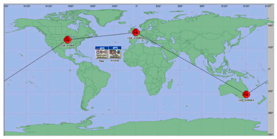
Figure 10.
CGE Iowa-CGE London-CGE Sidney Riverbed scenarios following the structure.
- L–I: GCE London to GCE Iowa (Bandwidth of 1 Gbps; latency of 45 ms)
- S–I: GCE Sidney to GCE Iowa (Bandwidth of 1 Gbps; latency of 85 ms)
- S–L: GCE Sidney to GCE London (Bandwidth of 1 Gbps; latency of 130 ms).
Once the test environment is defined and emulated, the tests are deployed following Pantheon’s methodology. This methodology consists of launching the same test five times over the three scenarios. Each test lasts for 30 s, running three flows using the same protocol with 10-s interval between two flows. The performance metrics results consider the three flows and average the results of the five runs. The performance metrics to be evaluated are the Average of the throughput achieved in percentage (29), the Delay Ratio (30), and the Packet Loss Ratio (PLR).
In the case of the delay, the Delay Ratio is used, which is the average one-delay achieved related with the minimum one-way delay in order to check the introduced delay in the network by each protocol.
For the Packet Loss Ratio (%), the lost packets sent are related to the total packets sent. This metric reflects the effects of the load produced by the three coexisting protocol flows that are trying to reach the maximum bandwidth.
The first metric for the performance comparison is the throughput (Figure 11). From this graph, it can be extracted that the Enhanced-AATP achieves a mean throughput of the 80% of the bandwidth, providing better performance than most of the protocols. Similar behavior can be checked with TCP-Cubic, but performance decreases as the delay increases. BBR reaches better results, but these results are over the maximum bandwidth, which means that the protocol might be destabilizing the network.
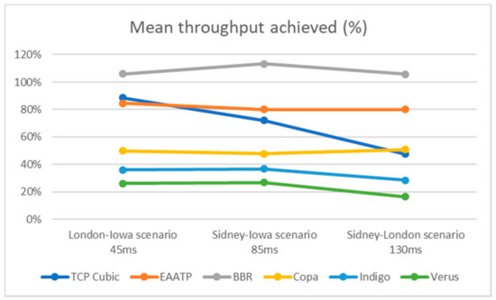
Figure 11.
Mean throughput achieved (%) comparison.
In order to check how the throughput performance affects the network, the following figure (Figure 12) shows the Delay Ratio (average delay achieved compared with the minimum delay). In the case of the Enhanced-AATP, the delay introduced by the protocol is around 25% (1.25), which means that the network is stable. It can be seen that BBR destabilizes the network because its one-way delay multiplies per 4 the latency of the network in the lower delay scenario. Similar behavior can be seen with TCP Cubic, which doubles the one-way delay of the network (2.00) in the lower delay scenario.
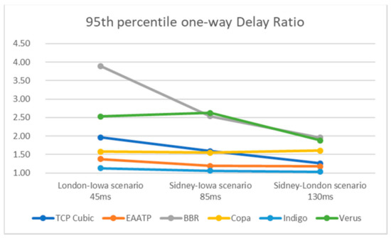
Figure 12.
95th percentile one-way Delay Ratio comparison.
The Packet Loss Ratio is checked in Figure 13 in order to confirm the effects of the protocols’ behavior regarding the throughput and the delay. The losses introduced by the Enhanced-AATP are low (0.02%), as it happens with the most of the protocols. It is confirmed that BBR achieves better throughput to the detriment of the introduced losses (from 3% to 7%).
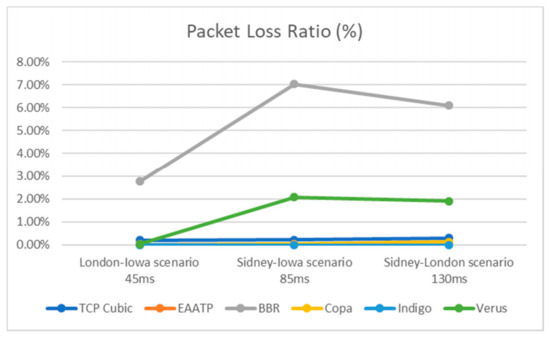
Figure 13.
Packet Loss Ratio (%) comparison.
Finally, with the information provided by the last three figures, the following graph (Figure 14) shows the protocols’ performance for each scenario, relating the 95th percentile one-way Delay Ratio and the Average Throughput achieved. Moreover, the Packet Loss Ratio is noted. This relativized view of the data enables us to contrast the protocols’ performance joining the three scenarios’ results. The objective is to provide a final performance comparison of the Enhanced-AATP with these protocols: TCP Cubic, BBR, Copa, Indigo, and Verus.
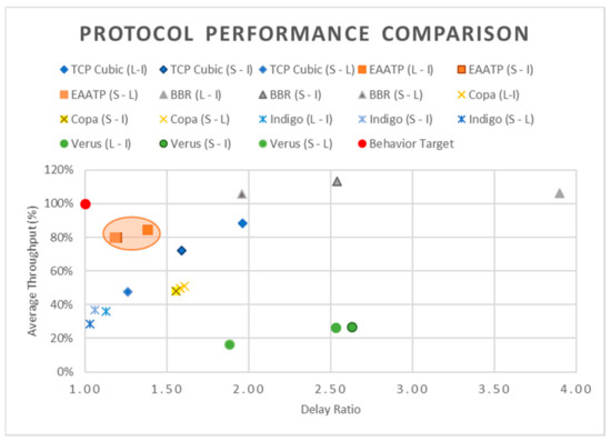
Figure 14.
Protocol Performance Comparison (Throughput–Delay Ratio) over the three scenarios. Packet Loss Ratio (PLR) is noted. TCP Cubic: 0.24%; Enhanced-AATP: 0.02%; BBR: 5.30%; Copa: 0.06%; Indigo: 0.00%; Verus: 1.33%; Behavior Target: 0.00%.
The goal is to achieve the maximum throughput without affecting the delay neither causing losses. The Behavior Target (red circle) is the ideal protocol that achieves maximum throughput levels (100%) without affecting the congestion of the network (minimum one-way delay) nor generating losses during the data transfer. For the best performance, the protocols have to tend to the aforementioned behavior. Among the studied protocols, as the orange circle highlights, the Enhanced-AATP protocol achieves a high average throughput (80%) without destabilizing the network by slightly increasing (25%) the latency neither causing significant losses (0.02%).
Comparing the Enhanced-AATP with low delay protocols such as Indigo, the Enhanced-AATP obtains a greater throughput (Average Throughput: Indigo (35%)—Enhanced-AATP (82%)) causing a slightly increase of the delay (Delay Ratio: Indigo (1.1)—Enhanced-AATP (1.4)) without provoking significant losses (PLR: Indigo (0.00%)—Enhanced-AATP (0.02%)).
Moreover, comparing the Enhanced-AATP with high bandwidth protocols as BBR, the Enhanced-AATP does not reach that levels of throughput (Average Throughput: BBR (110%)—Enhanced-AATP (82%)) but has a stable behavior without strongly increasing the latency (Delay Ratio: BBR (2.8)—Enhanced-AATP (1.4)) and causing losses (PLR: BBR (5.30%)—Enhanced-AATP (0.02%)).
It can be concluded that the Enhanced-AATP protocol achieves the goal. The protocol maintains its throughput close to the limit without destabilizing the network thanks to the Bandwidth Estimation process, the LTD mechanism, and its operation states, which modify the Sending Rate depending on the network situation (Table 3). In addition, the Weighted Fairness mechanism provides a fairly controlled share of the network resources among the flows without causing significant losses due to the dispute of the bandwidth.
7. Conclusions
In this paper, we propose the Enhanced-AATP transport protocol as an improvement of the Aggressive and Adaptative Transport Protocol (AATP), which aims to modify operations and add new functionalities to achieve improved performance over fairly shared heterogeneous Long Fat Networks. One of these functionalities ensures the differentiation of the type of loss episode (congestion or channel), which then proposes a corresponding operation to solve the different types of loss. Moreover, a prioritized fair share of the network resources when multiple AATP flows are connected to the same node is achieved thanks to the new Weighted Fairness mechanism.
After analyzing the different proposals of distinct transport protocols, their metrics and mechanisms for wireless networks, the smooth Jitter Ratio () is the reference metric chosen to distinguish the type of losses. The relates the effect of the queued packets at the bottleneck and the delay among packets at the destination, also considering past values of the Jitter Ratio. This metric is not affected by the high delay introduced in the LFNs.
Having selected the Jitter Ratio metric, the Loss Threshold Decision maker (LTD) is designed. It is defined as the added number of packets in the burst over the total packet sent in the burst. By comparing it with the smooth Jitter Ratio () of the received packets, the result of this comparison enables the protocol to discern between losses caused by network congestion or channel fault.
If the is greater or equal to , a congestion loss occurs; if the is lower than the , it is assumed that a channel failure caused the loss. As a result of this loss detection mechanism, the throughput is not reduced during a random loss episode, as it occurs during a congestion loss episode, thus reducing the loss recovery time and increasing the efficiency of the protocol.
The performance of the Enhanced-AATP and its operation over wireless connections is shown, as well as its capability to detect a random loss produced by the channel. Similarly, the capacity of the protocol to decide the type of loss occurred is exhibited over different scenarios. Finally, the optimal value of the is demonstrated. All the experiments are deployed over the SteelCentral Riverbed Modeler simulator.
As a result of studying different indicators for a controlled fair share of the network resources of a node, the Jain Fairness Index (JFI) is chosen due to its characteristics and compliance with the requirements demanded. After adapting the JFI to consider the prioritization of the flows, the Weighted Fairness (WF) index is included in the operation of the Enhanced-AATP protocol. If the WF is equal to 1, it means that there is a fair share of resources; if not, it means that some unfair treatment is happening to one or more flows. Therefore, the protocol operation is adjusted to include a modifier related to the result of the WF to manage the flows for a fair system. Different simulations are run with different priorities and flows to demonstrate its performance. The WF suffers fluctuations during the beginning or end of a new flow.
It can be concluded that the Enhanced-AATP can effectively differentiate the types of losses occurred during a communication, adapting its operation to the situation, and assuring a fair sharing of the resources of the node over HLFNs.
Finally, the Enhanced-AATP’s performance is compared with other transport protocols’ performance. It should be highlighted that the protocol reaches a higher throughput than low delay protocols, slightly increasing the delay but keeping a similar low level of losses. Moreover, compared with high bandwidth protocols, the Enhanced-AATP reaches lower throughput levels (>80%) but does not destabilize the network, nor does it highly increase the latency (+25%) or cause significant losses (0.02%) as may occur with other protocols. This high performance is the result of including the proposed Loss Threshold Decision maker (in order to identify the type of losses occurred) and the Weighted Fairness mechanisms (fairly share of the server network resources) in the improved AATP operation, which modifies its behavior and, concretely, its Sending Rate depending on the network situation.
Our future work aims to introduce a way to detect the loss and recovery of the channel by way of preventing unnecessary packet transfers in order to save energy, and a method to create a distributed fairness system, as opposed to one that is controlled by the node where different Enhanced-AATP flows coexist. Finally, an exhaustive analysis of the relationship of the and parameters of the Transcendence Factor (A) can be done to study its optimal performance and convergence.
Author Contributions
Conceptualization, A.B. and A.Z.; methodology, A.B. and A.M.; software, A.M.; validation, A.Z. and R.M.d.P.; formal analysis, A.B. and R.M.d.P.; investigation, A.B., R.M.d.P. and A.M.; resources, A.Z.; data curation, A.M.; writing—original draft preparation, A.B.; writing—review and editing, A.Z., R.M.d.P. and A.M.; visualization, A.M.; supervision, A.Z.; project administration, A.B. All authors have read and agreed to the published version of the manuscript.
Funding
This research received no external funding.
Acknowledgments
This article in journal has been possible with the support from the “Secretaria d’Universitats i Recerca del Departament d’Empresa i Coneixement de la Generalitat de Catalunya”, the European Union (EU) and the European Social Fund (ESF) [2020 FI_B 00448]. The authors would like to thank “La Salle-URL” (University Ramon Llull) for their encouragement and assistance. This work received support from the “Agència de Gestió d’Ajuts Universitaris i de Recerca (AGAUR)” of “Generalitat de Catalunya” (grant identification “2017 SGR 977”).
Conflicts of Interest
The authors declare no conflict of interest.
References
- Cisco. Cisco Annual Internet Report (2018–2023). Available online: https://www.cisco.com/c/en/us/solutions/collateral/service-provider/visual-networking-index-vni/white-paper-c11-741490.html (accessed on 25 January 2021).
- Naghshineh, M.; Schwartz, M.; Acampora, A.S. Issues in Wireless Access Broadband Networks. In The International Series in Engineering and Computer Science; Springer Science and Business Media: Berlin/Heidelberg, Germany, 1996; Volume 351, pp. 1–19. [Google Scholar]
- Jacobson, V.; Braden, R.; LBL; ISI. TCP Extensions for Long-Delay Paths, IETF. 1988. Available online: https://tools.ietf.org/html/rfc1072 (accessed on 20 April 2021).
- Cerf, V.; Kahn, R. A Protocol for Packet Network Intercommunication. IEEE Trans. Commun. 1974, 22, 637–648. [Google Scholar] [CrossRef]
- Fieger, A.; Zitterbart, M. Transport protocols over wireless links. In Proceedings of the Second IEEE Symposium on Computer and Communications, Alexandria, Egypt, 1–3 July 1997; pp. 456–460. [Google Scholar] [CrossRef]
- Xylomenos, G.; Polyzos, G.C. TCP and UDP performance over a wireless LAN. In Proceedings of the INFOCOM’99—Eighteenth Annual Joint Conference of the IEEE Computer and Communications Societies, New York, NY, USA, 21–25 March 1999; pp. 439–446. [Google Scholar] [CrossRef]
- Shenoy, S.U.; Kumari, M.S.; Shenoy, U.K.K.; Anusha, N. Performance analysis of different TCP variants in wireless ad hoc networks. In Proceedings of the 2017 International Conference on I-SMAC (IoT in Social, Mobile, Analytics and Cloud) (I-SMAC), Palladam, India, 11–12 February 2017; pp. 891–894. [Google Scholar] [CrossRef]
- Chaudhary, P.; Kumar, S. Comparative study of TCP variants for congestion control in wireless network. In Proceedings of the 2017 International Conference on Computing, Communication and Automation (ICCCA), Greater Noida, India, 5–6 May 2017; pp. 641–646. [Google Scholar] [CrossRef]
- Tian, Y.; Xu, K.; Ansari, N. TCP in wireless environments: Problems and solutions. IEEE Commun. Mag. 2005, 43, S27–S32. [Google Scholar] [CrossRef]
- Xylomenos, G.; Polyzos, G.C.; Mahonen, P.; Saaranen, M. TCP performance issues over wireless links. IEEE Commun. Mag. 2001, 39, 52–58. [Google Scholar] [CrossRef]
- Mammadov, A.; Abbasov, B. A review of protocols related to enhancement of TCP performance in wireless and WLAN networks. In Proceedings of the 2014 IEEE 8th International Conference on Application of Information and Communication Technologies (AICT), Astana, Kazakhstan, 15–17 October 2014; pp. 1–4. [Google Scholar] [CrossRef]
- El-Bazzal, Z.; Ahmad, A.M.; Houssini, M.; El Bitar, I.; Rahal, Z. Improving the performance of TCP over wireless networks. In Proceedings of the 2018 Sixth International Conference on Digital Information, Networking, and Wireless Communications (DINWC), Beirut, Lebannon, 25–27 April 2018; pp. 12–17. [Google Scholar] [CrossRef]
- Mishra, N.; Verma, L.P.; Kumar, M. Comparative Analysis of Transport Layer Congestion Control Algorithms. In Proceedings of the 2019 International Conference on Cutting-edge Technologies in Engineering (ICon-CuTE), Uttar Pradesh, India, 14–16 November 2019; pp. 46–49. [Google Scholar] [CrossRef]
- Briones, A.; Mallorquí, A.; Zaballos, A.; De Pozuelo, R.M. Adaptive and aggressive transport protocol to provide QoS in cloud data exchange over Long Fat Networks. Future Gener. Comput. Syst. 2021, 115, 34–44. [Google Scholar] [CrossRef]
- Riverbed Modeler. Available online: https://www.riverbed.com/gb/products/steelcentral/steelcentral-riverbed-modeler.html (accessed on 25 January 2021).
- Shchapov, V.; Masich, G.; Masich, A. Platform for Parallel Processing of Intense Experimental Data Flow on Remote Supercomputers. Procedia Comput. Sci. 2015, 66, 515–524. [Google Scholar] [CrossRef][Green Version]
- Jacobson, V. Congestion avoidance and control. ACM SIGCOMM Comput. Commun. Rev. 1988, 18, 314–329. [Google Scholar] [CrossRef]
- Shi, H.; Prasad, R.V.; Onur, E.; Niemegeers, I.G.M.M. Fairness in Wireless Networks: Issues, Measures and Challenges. IEEE Commun. Surv. Tutor. 2013, 16, 5–24. [Google Scholar] [CrossRef]
- Dong, M.; Li, Q.; Zarchy, D.; Godfrey, P.B.; Schapira, M. {PCC}: Re-architecting congestion control for consistent high performance. In Proceedings of the 12th {USENIX} Symposium on Networked Systems Design and Implementation ({NSDI} 15), Oakland, CA, USA, 4–6 May 2015; pp. 395–408. [Google Scholar]
- Fu, C.P.; Liew, S. TCP Veno: TCP enhancement for transmission over wireless access networks. IEEE J. Sel. Areas Commun. 2003, 21, 216–228. [Google Scholar] [CrossRef]
- Brakmo, L.; Peterson, L. TCP Vegas: End to end congestion avoidance on a global Internet. IEEE J. Sel. Areas Commun. 1995, 13, 1465–1480. [Google Scholar] [CrossRef]
- Takagaki, K.; Ohsaki, H.; Murata, M. Analysis of a window-based flow control mechanism based on TCP Vegas in heterogeneous network environment. In Proceedings of the IEEE International Conference on Communications. Conference Record (Cat. No.01CH37240), Helsinki, Finland, 11–14 June 2001; pp. 3224–3228. [Google Scholar] [CrossRef]
- Dong, P.; Wang, J.; Huang, J.; Wang, H.; Min, G. Performance Enhancement of Multipath TCP for Wireless Communications With Multiple Radio Interfaces. IEEE Trans. Commun. 2016, 64, 3456–3466. [Google Scholar] [CrossRef]
- El-Ocla, H. TCP CERL: Congestion control enhancement over wireless networks. Wirel. Netw. 2008, 16, 183–198. [Google Scholar] [CrossRef]
- Saedi, T.; El-Ocla, H. Performance analysis of TCP CERL in wireless networks with random loss. In Proceedings of the 2019 IEEE Canadian Conference of Electrical and Computer Engineering (CCECE), Edmonton, AB, Canada, 5–8 May 2019; pp. 1–4. [Google Scholar] [CrossRef]
- Saedi, T.; El-Ocla, H. TCP CERL+: Revisiting TCP congestion control in wireless networks with random loss. Wirel. Netw. 2020, 1–18. [Google Scholar] [CrossRef]
- Mascolo, S.; Casetti, C.; Gerla, M.; Sanadidi, M.Y.; Wang, R. TCP westwood. In Proceedings of the 7th Annual International Conference on Mobile Computing and Networking, New York, NY, USA, 19–23 July 2011; pp. 287–297. [Google Scholar] [CrossRef]
- Grieco, L.A.; Mascolo, S. Performance evaluation and comparison of Westwood+, New Reno, and Vegas TCP congestion control. ACM SIGCOMM Comput. Commun. Rev. 2004, 34, 25–38. [Google Scholar] [CrossRef]
- Joe, I.; Lee, J. An Enhanced TCP Protocol for Wired/Wireless Networks. In Proceedings of the 2009 Fifth International Joint Conference on INC, IMS and IDC, Seoul, Korea, 25–27 August 2009; pp. 531–533. [Google Scholar] [CrossRef]
- Kanagarathinam, M.R.; Singh, S.; Sandeep, I.; Roy, A.; Saxena, N. D-TCP: Dynamic TCP congestion control algorithm for next generation mobile networks. In Proceedings of the 2018 15th IEEE Annual Consumer Communications & Networking Conference (CCNC), Las Vegas, NV, USA, 12–15 January 2018; pp. 1–6. [Google Scholar] [CrossRef]
- Arun, V.; Balakrishnan, H. Copa: Practical Delay-Based Congestion Control for the Internet. In Proceedings of the ANRW’18: Applied Networking Research Workshop, New Montreal, QC, Canada, 9–11 April 2018; p. 19. [Google Scholar] [CrossRef]
- Zaki, Y.; Pötsch, T.; Chen, J.; Subramanian, L.; Görg, C. Adaptive Congestion Control for Unpredictable Cellular Networks. ACM SIGCOMM Comput. Commun. Rev. 2015, 45, 509–522. [Google Scholar] [CrossRef]
- Cardwell, N.; Cheng, Y.; Gunn, C.S.; Yeganeh, S.H.; Jacobson, V. BBR. Commun. ACM 2017, 60, 58–66. [Google Scholar] [CrossRef]
- Grazia, C.A.; Klapez, M.; Casoni, M. BBRp: Improving TCP BBR Performance Over WLAN. IEEE Access 2020, 8, 43344–43354. [Google Scholar] [CrossRef]
- Li, T.; Zheng, K.; Xu, K.; Jadhav, R.; Xiong, T.; Winstein, K.; Tan, K. TACK: Improving Wireless Transport Performance by Taming Acknowledgments. In Proceedings of the Annual Conference of the ACM Special Interest Group on Data Communication on the Applications, Technologies, Architectures, and Protocols for Computer Communication (SIGCOMM’20), Virtual Event, New York, NY, USA, 10–14 August 2020; pp. 15–30. [Google Scholar] [CrossRef]
- Wu, E.-K.; Chen, M.-Z. JTCP: Jitter-Based TCP for Heterogeneous Wireless Networks. IEEE J. Sel. Areas Commun. 2004, 22, 757–766. [Google Scholar] [CrossRef]
- Chen, J.-M.; Chu, C.-H.; Wu, E.H.-K.; Tsai, M.-F.; Wang, J.-R. Improving SCTP Performance by Jitter-Based Congestion Control over Wired-Wireless Networks. EURASIP J. Wirel. Commun. Netw. 2011, 2011, 103027. [Google Scholar] [CrossRef]
- Xu, K.; Tian, Y.; Ansari, N. TCP-Jersey for Wireless IP Communications. IEEE J. Sel. Areas Commun. 2004, 22, 747–756. [Google Scholar] [CrossRef]
- Reddy, V.B.; Sarje, A.K. Differentiation of Wireless and Congestion Losses in TCP. In Proceedings of the 2007 2nd International Conference on Communication Systems Software and Middleware, Bangalore, India, 7–12 January 2007; pp. 1–5. [Google Scholar] [CrossRef]
- Yan, F.Y.; Ma, J.; Hill, G.D.; Raghavan, D.; Wahby, R.S.; Levis, P.; Winstein, K. Pantheon: The training ground for internet congestion-control research. In Proceedings of the 2018 USENIX Conference on Usenix Annual Technical Conference (USENIX ATC’18), Berkeley, CA, USA, 11–13 July 2018; pp. 731–743. [Google Scholar] [CrossRef]
- Pantheon. Available online: https://pantheon.stanford.edu/ (accessed on 25 January 2021).
- Bhatti, S.; Bateman, M. Transport Protocol Throughput Fairness. J. Netw. 2009, 4, 881–894. [Google Scholar] [CrossRef]
- Kim, G.-H.; Song, Y.-J.; Cho, Y.-Z. Improvement of inter-protocol fairness for BBR congestion control using machine learning. In Proceedings of the 2020 International Conference on Artificial Intelligence in Information and Communication (ICAIIC), Fukuoka, Japan, 19–21 February 2020; pp. 501–504. [Google Scholar] [CrossRef]
- Wang, C. Achieving per-flow and weighted fairness for uplink and downlink in IEEE 802.11 WLANs. EURASIP J. Wirel. Commun. Netw. 2012, 2012, 239. [Google Scholar] [CrossRef]
- Shi, H. Fairness and Resource Allocation in Device-to-Device Wireless Regional Area Network. Ph.D. Thesis, TU Delft, Delft, The Netherlands, 2014. [Google Scholar] [CrossRef]
- Köppen, M.; Ohnishi, K.; Tsuru, M.; Ohnishi, K. Multi-Jain Fairness Index of Per-Entity Allocation Features for Fair and Efficient Allocation of Network Resources. In Proceedings of the 2013 5th International Conference on Intelligent Networking and Collaborative Systems, Xi’an, China, 9–11 September 2013; pp. 841–846. [Google Scholar] [CrossRef]
- Gu, Y.; Grossman, R.L. UDT: UDP-based data transfer for high-speed wide area networks. Comput. Netw. 2007, 51, 1777–1799. [Google Scholar] [CrossRef]
- Gu, Y.; Hong, X.; Grossman, R. An Analysis of AIMD Algorithm with Decreasing Increases. Available online: https://www.researchgate.net/publication/238691040_An_Analysis_of_AIMD_Algorithm_with_Decreasing_Increases (accessed on 25 January 2021).
- Jindal, A.; Psounis, K. On the Efficiency of CSMA-CA Scheduling in Wireless Multihop Networks. IEEE/ACM Trans. Netw. 2012, 21, 1392–1406. [Google Scholar] [CrossRef]
- Jay, N.; Rotman, N.; Godfrey, B.; Schapira, M.; Tamar, A. A Deep Reinforcement Learning Perspective on Internet Congestion Control. In Proceedings of the 36th International Conference on Machine Learning, Long Beach, CA, USA, 9–15 June 2019; pp. 3050–3059. Available online: http://proceedings.mlr.press/v97/jay19a.html (accessed on 20 April 2021).
- Dong, M.; Meng, T.; Zarchy, D.; Arslan, E.; Gilad, Y.; Godfrey, P.; Schapira, M. PCC vivace: Online-learning congestion control. In Proceedings of the 15th USENIX Conference on Networked Systems Design and Implementation (NSDI’18), Renton, WA, USA, 9–11 April 2018; pp. 343–356. [Google Scholar] [CrossRef]
Publisher’s Note: MDPI stays neutral with regard to jurisdictional claims in published maps and institutional affiliations. |
© 2021 by the authors. Licensee MDPI, Basel, Switzerland. This article is an open access article distributed under the terms and conditions of the Creative Commons Attribution (CC BY) license (https://creativecommons.org/licenses/by/4.0/).