Valuation of Wind Energy Turbines Using Volatility of Wind and Price

Abstract

The limitedness of the nonrenewable local energy resources in Israel, even in the background of the later gas fields’ findings, continues to force the state to devote various efforts towards ‘green’ energy development. These efforts include installations, both for the solar and for wind energy, thus improving the diversity of energy sources. While the standard discounted cash flow (DCF) method using the net present value (NPV) criterion is extensively adopted to evaluate investments, the standard DCF method is inappropriate for the rapidly changing investment climate and for the managerial flexibility in investment decisions. In recent years, the real options analysis (ROA) technique has been widely applied in many studies for the valuation of renewable energy investment projects. Taking into account the above background, we apply, in this study, the real options analysis approach for the valuation of wind energy turbines and apply it to the analysis of wind energy economic potential in Israel, which is the context of our work. We hypothesize that due to nature of wind energy production uncertainties, the ROA method is better than the alternative. The novelty of this paper includes the following: real world wind statistics of the Merom Golan site in Israel (velocity 3.73 m/s, with a standard deviation of 2.03 m/s), a realistic power generation estimation (power generation of 1205.84 kW with a standard deviation of about 0.5% in annual value which is worth about 1.3 M$ per annum), and an economic model to evaluate the profitability of such a project. We thus discuss the existing challenges of diversifying renewable energy sources in Israel by adding wind installations. Our motivation is to introduce a method which will allow investors and officials to take into account uncertainties when deciding in investing in such wind installations. The outcomes of the paper, which are obtained using the method of Weibull statistics and the Black–Scholes ROA technique, include the result that market price volatility adds to the uncertainties much more than any wind fluctuations, provided that the analysis is integrated over a long enough time.

1. Introduction

Even during prolonged global economic crisis, the worldwide wind power ascent continues. The world’s wind power capacity, according to the Global Wind Energy Council (GWEC) report, added 39.1 GW in 2010, growing by 24% during the year, 40.6 GW in 2011, growing by 20.5% per year, and 44.8 GW in 2012 (18.8% growth during the year: 78% growth in the last three years). Thus, the total installations at the end of 2012 provide up to 282.6 GW. A huge part of this power was produced in China—first place globally, with 75.3 GW, or 26.7% of the world product (about 30% of the world year’s additions), the and USA—60.0 GW, or 21.2% of the world product, while Germany, Spain, and India (3rd–5th places) produced 25.7% together [1].

Wind energy is now a significant participant in the world’s energy market. The 2012 global wind power market grew by more than 10% compared to 2011, representing investments of about 56 billion €. The main markets of wind energy are situated in Asia, North America, and Europe, each of which installs 13–15 GW of new capacity each year. About half a million people are now employed, corresponding to the European Wind Energy Association (EWEA) publication, by the wind industry around the world [2].

Considering the growing Israeli energy market, even nowadays, when plentiful sources of traditional nonrenewable energy such as the vast gas fields that were found in the Mediterranean Sea off the coast of Israel, Tamar (Tamar gas field [3]), and Leviathan (Leviathan gas field [4]), with the estimated quantity of 356 and 450 billion cubic meters, respectively, the possibility of their exhaustion still forces the state, as other numerous political entities, to devote significant efforts towards ‘green’ energy research and development. This is also important from the point of view of reducing carbon emission and global warming. These efforts are undertaken primarily for developing solar energy, but also recently for wind energy facilities. Yet, the wind power amount produced in Israel is rather small compared to the continuously growing global market; however, the recent steps undertaken by the state are destined to make the situation better.

Israel currently operates a wind farm in Asanyia mountain in the Golan Heights with an installed capacity of 6 MW (10 turbines reaching a height 50 m (blades included), each with a power capacity of 600 kW), this is the typical consumption of about five thousand families. The duty cycle of the wind farm reaches 97%, and electricity production is worth 1 million US$ a year. Indeed, the wind energy potential of Israel is rather restricted due to moderate or poor wind velocities in most areas and the restricted number of areas with high average wind speed. In many areas worthy of wind energy development, one is encountered by the opposition of green groups on landscape conservation grounds and the influence of the facility on local and migrating birds. Nevertheless, satisfying the Israel Ministry of Environmental Protection (IMEP) directions, the state of Israel continues efforts towards the development of additional farms with a 50 MW capacity [5].

As it is emphasized in a document issued by the Israeli Parliament (Knesset), a better estimate, based on the wind turbines’ technical development, gives a value of more than 500 MW for the Israeli potential wind energy potential capacity [6]. One of the prospective areas for the development of efficient wind technology, considering its climatic characteristics, is the region of Ariel city in Samaria [7], the current research, however, is devoted to another region [8].

While the generic discounted cash flow (DCF) approach using the net present value (NPV) criterion is generally adopted to evaluate investments, the DCF method is inappropriate for a rapidly changing investment situation (Dixit and Pindyck [9]; Herath and Park [10]; Lee and Shih [11]) and does not consider managerial flexibility in investment decisions (Hayes and Abernathy [12]; Hayes and Garvin [13]; Trigeorgis and Mason [14]; Trigeorgis [15]). In the current study, we consider a two-stage approach—one turbine at the first stage and a field of 50 at the second stage, along with the possibility to withdraw at the second stage. Hence, the scenario is a one in which managerial flexibility can be practiced.

Currently, the real option analysis method is widely applied in many studies for the valuation of renewable energy investment projects, for example, Lee and Shih [11] and Kumbaroğlu, Madlener, and Demirel [16]. See also Boomsma, Meade, and Fleten [17] and Menegaki [18]. We thus apply in this paper the real options analysis method for the evaluation of the economic value of wind energy turbines in a specific location. In particular, we analyze the value of the investment opportunities that add value to the investment due to managerial flexibility (in the case of energy market price drop, one may abandon the investment). It is worth mentioning that the option valuation method has become more sophisticated by using approaches such as the binomial lattice, the mean reverting jump-diffusion method, and stochastic volatility model. It is also used for other types of hazards such as technological risks (Deng [18]; Menegaki [19]; Siddiqui, Marnay, and Wiser [20]), which may include a change in the wind regime, in our case, or power output reduction of the turbine. See also Davis and Owens [21] and Baringo and Conejo [22].

The reasons for the current study are as follows, we are interested in estimating the profitability of a Merom Golan wind facility. For this:

(1)

We calculate the revenue from Merom Golan due to electric energy production.

(2)

We show that, taking into account the annual energy production, fluctuations are rather small; this is contrasted with rather large fluctuations when one considers the data over a daily basis.

(3)

This is then integrated into two economic models; one is the standard discounted cash flow and the other is the real options analysis.

(4)

We finally show that, because of energy price volatility and despite small technical fluctuations, the correct estimation of the investment is given by the real options analysis, which takes into account the ability of the investors to abort their investment after the first stage.

The main purpose of this paper is to study the effect of energy value fluctuations on the assessment of the profitability of wind turbine facilities using the real option analysis method. The economic output of a wind turbine installation is a function of its electric energy output [23,24,25] and the value of market energy. The electric energy output is a function of the turbine used and wind speed statistics. The turbine used can be chosen to have an optimal cut-in velocity (the wind speed level at which the turbine starts to generate electricity), and the cut-out velocity (the speed level at which the facility hits its alternator limit and stops producing more power output following increases in wind velocity) [26]. For a more technical discussion, we refer the reader to the results of our previous studies on wind power production, devoted to the technological appropriateness and environmental relevance issues [7,27]. See also [28,29]. While the total annual energy output of the turbine facility can be known to a high certainty, the market prices of energy may vary indeterminately, and thus should be considered as the most serious investment risk. To evaluate the financial risk correctly, we suggest employing the real option analysis method, which is the subject of the current study. In a wider sense, our manuscript contributes to the risk analysis of Grossman, which is the way a “decentralized economy allocates risk and investment resources when information is dispersed” [30] (p. 773).

In this paper, we shall describe the various sources of the uncertainties in determining the economic value of a wind installation. Both in terms of technical parameters, such as wind velocity change, and the effect on the power output of the turbine. Additionally, in terms of the market value of the power generated, which is dependent on the value of competing power generation methods. We then combine the uncertainties to produce the economic value of the installation using the real option analysis evaluation techniques. On comparing the different sources of uncertainty, we show that the uncertainty in the market value of electric power significantly dominates the technical uncertainties.

The structure of the paper is as follows: in the “Materials and Methods” section we describe the methods of this work, which are the Weibull statistics of wind and the Black–Scholes analysis of the real option technique. In the “Results” section we describe the Weibull fit for the site of installation, deriving the relevant parameters; we also introduce the economic model in terms of its parameters and emphasize the difference between the DCF and ROA methods for evaluation. Next, in the “Discussion” section, we estimate the power production and power uncertainty for different turbines and compare this with the economic uncertainty of energy prices, determining that the latter is much larger. Finally, in the “Conclusion” section, we summarize our conclusions underlining the dominance of market price fluctuations over technical fluctuations and the benefit of using the ROA method over the DCF method for a better economic evaluation of the wind energy facility expedience.

2. Materials and Methods

In this study we concentrated on the wind speed distribution in the Golan heights area, using the information available from the meteorological service of the Israel Ministry of Transport [31], gathered by the Merom Golan meteorological station, one of the 84 Israeli meteorological facilities, which is situated at the relevant area [32], for the year 2014. The file used includes 52,066 data points gathered during the specified period. This includes sample values of the wind speed, one observation for every 10 min or 144 values per day (except for some non-significant missing values) [33]. We describe the data analytically using the Weibull probability density function (PDF). This is commonly accepted as the most appropriate function describing the wind speed statistical frequencies at a given location in most world locations. These data are essential for the planning of the wind turbine optimal choice [7].

The Weibull PDF is determined, in addition to a random variable X, representing here the wind speed, by two parameters, which are location dependent. They are a shape parameter k (dimensionless) and a scale parameter λ (m/s for the wind speed), which, together, determine the following PDF form:

$$f\left(x;\lambda ,k\right)=\left\{\begin{array}{ll}\frac{k}{\lambda }{\left(\frac{x}{\lambda }\right)}^{k-1}{e}^{-{\left(\frac{x}{\lambda }\right)}^k},& x\ge 0\\ 0,& x=0\end{array}\right.$$

Both PDF parameters are important for choosing the best location for the appropriate wind turbine, which imply the wind farm’s economic value [34].

The wind velocity determines the electric power output. We will evaluate the power output based on wind statistics and turbine characteristics in the results section. As the electric power is sold to the users, the remaining question in evaluating the value of the installation is how much money the user will pay for their power consumption, in other words, “what is the market value of the power?”, which reflects on the economic value of the installation. In the following, we describe the methods used for such evaluation.

While the generic discounted cash flow (DCF) approach using the net present value (NPV) criterion is generally adopted to evaluate investments, the DCF method is inappropriate for a rapidly changing investment situation (Dixit and Pindyck [20]; Herath and Park [21]; Lee and Shih [11]) and does not consider managerial flexibility in investment decisions (Hayes and Abernathy [23]; Hayes and Garvin [24]; Trigeorgis and Mason [25]; Trigeorgis [26]). In the current study, we consider a two-stage approach—one turbine at the 1st stage and a field of 50 at the 2nd stage; along with the possibility to withdraw at the 2nd stage. Hence, the scenario is a one in which managerial flexibility can be practiced.

Currently, the real option analysis method is widely applied in many studies for the valuation of renewable energy investment projects, for example Lee and Shih [11] and Kumbaroğlu, Madlener, and Demirel [27]. See also Boomsma, Meade, and Fleten [28] and Menegaki [29]. We thus apply in this paper the real options analysis method for the evaluation of the economic value of wind energy turbines in a specific location. In particular, we analyze the value of the investment opportunities that add value to the investment due to managerial flexibility (in the case of energy market price drop, one may abandon the investment). It is worth mentioning that the option valuation method has become more sophisticated by using approaches such as the binomial lattice, the mean reverting jump-diffusion method, and stochastic volatility model. It is also used for other types of hazards such as technological risks (Deng [30], Menegaki [29], Siddiqui, Marnay, and Wiser [31]), which may include a change in the wind regime, in our case, or power output reduction of the turbine. See also Davis and Owens [32] and Baringo and Conejo [33].

However, we decided to adopt the basic Black–Scholes equation of a financial market [35] because we were focused on the underestimated value of the option to abort the investment in an environment where it is not possible to foresee the standard deviation using numerical tools.

In this study, we analyzed the possibility of installing additional turbines in the Asanyia mountain in the Golan Heights in order to extract profit from wind-generated power. We have partly based our study on the known results of wind turbine construction and use in Israel [36], while part of the numbers presented here are rather rough estimates. The decision to construct a field, which is a collection of many turbines, can be divided into two stages: in the 1st stage we build one unit. After building and operating this single unit for few years and gaining confidence in the technical and financial output, the 2nd stage, regarding the decision of building the entire turbine field, is made, based on electricity price at this stage as well as the future predicted energy evaluation.

We evaluate the uncertainty over future electricity market price as an economic value of an underlying asset of a real option using the Black–Scholes equation [35]:

$$C=S_0 N\left(d_1\right)-K e^{-rT}N\left(d_2\right)$$

where

$$\begin{array}{l}{d}_1=\frac{\ln (S_0/K) + \left(r + {\sigma }^2/2\right)T}{\sigma \sqrt{T}},\\ d_2=\frac{\ln (S_0/K) + \left(r - {\sigma }^2/2\right)T}{\sigma \sqrt{T}}=d_1-\sigma \sqrt{T}.\end{array}$$

We use the following notations: C is the call option value, S₀ is the market price of the underlying asset, K is the exercise price, r is the annual risk-free return, T is the duration of the period (the number of years) till exercising the real option (constructing the entire turbine field), and σ is the annualized standard deviation (StD) of the return of the underlying asset. N is the symbol of the Gaussian cumulative probability density function (CDF).

3. Results

3.1. Wind Energy Statistics

Several various methods exist for fitting the observed data of the given location [37] to the PDF. We used the method of the maximum likelihood estimators for PDF fitting [38]. The corresponding Weibull PDF for the wind speed distribution at the Merom Golan site, together with their distribution histogram, is shown below at Figure 1. (The authors are willing to share their data set in Excel format with those who wish to replicate the results of this research).

The figure demonstrates visually that low and moderate winds are widespread, with a tight condensation at the primary segment, which means that storms are just rare. It should be noticed that the distribution approximation by a Weibull PDF in this case is not perfect, although we could nevertheless obtain the wind principal statistical parameters approximately based on it.

Estimated annual parameters of the wind Weibull distribution were found to be k = 1.7228 and λ = 4.1206 m/s. In addition, we calculated (excess) kurtosis (a measure of the PDF sharpness) to be 2.1757, and skewness (a measure of the PDF asymmetry) as 0.0574, which were calculated to demonstrate the specific type of the Weibull PDF.

The main meaningful statistical parameter for the planning of the wind turbine installation, the speed mean, was obtained at 3.73 m/s, with standard deviation of 2.03 m/s, during the given period, with a positive right-skewed tail. This finding, in accordance with the Israeli Cooperative for Renewable Energy conclusions [39], indicates the possibility of wind energy exploitation in the investigated region.

3.2. Economical Model

All the used figures were elaborated in accordance with a proposed scenario as in

Table 1. Input data for the Black–Scholes option value calculation.

Data for the Black–Scholes Option Value
Cost of the first stage’s one turbine building	50
Annual turbine’s profit in the second stage	0.2
Present value of 50 turbines’ profit over 20 years = stock price now (S0)	114.7
Cost of the second stage for each turbine construction	1.2
Number of turbines in the second stage (entire field)	50
Cost of the second stage’s 50 turbines = exercise price of option (K)	60
Number of periods to exercise in years (T)	2
Compounded risk-free interest rate (r)	0.02
Standard deviation of prices of energy or electricity (annualized σ)	0.031

below, where the real figures can be introduced according to the data of each project (all prices are given in millions of US$):

We apply here the technique of real option valuation, as illustrated in Brealey et al. [40] (p. 584), where we have replaced:

(1)

The stock price with the current value of the field, S₀ = 114.7 million $US, which is the present value of 20 years of future operation with an annual profit of 0.2 million $US per turbine for a field of 50 turbines, discounted with 6% annual cost of capital;

(2)

The number of periods to exercise in years (T), with the number of years between the confirmation of the first stage (one unit) to the decision on the second stage (the field).

We have therefore calculated, at first, the call value, based on the annual StD estimation of 0.031, as 57.05 million $US. This StD estimation of 0.031 is based on the data of the Electric Power Monthly report of the U.S. Energy Information Administration (EIA), Table 5.3 “Average Retail Price of Electricity to Ultimate Customers” [41].

Our assumption of the first unit’s building cost is equal, as mentioned above, to 50 million $US, where such high expenses of the first turbine’s launching include, among others, research and development to adapt the turbine to the specific area under consideration and the cost of connecting it to the power grid, subtracted by the profit from operation.

We stress that the current work is based on assumed values, and, in this sense, it is an exercise in applying the real option technique. Future work will depend on a more realistic estimation of both the investment costs in infrastructure and current energy prices.

Hence, the results indicate that the investment in the first turbine stage is warranted, and the fact that there is the option to follow-on adds significant value to the investment. It follows that the net profit of the first stage is 57.05 − 50 = 7.05 million $US for the standard deviation value of 0.031, according to the following data of

Table 2. Intermediate and output data for the Black–Scholes option value.

Intermediate and Output Data for Two Assumptions on StD
StD	0.031	0.40
$\sigma \sqrt{T}$	0.0438	0.5657
d1	15.7146	1.4990
d2	15.6707	0.9333
Delta N(d1) Normal CDF	0.5123	0.9331
Value of the Call Option to Follow-On	57.05	59.48

(in a column for the case of StD = 0.031), which includes the intermediate values and the option to follow-on:

For comparison with a scenario lacking an option to abandon, the project value is estimated as the present discounted value of a difference between (i.e., the earnings from) the future cash flow raised from the second stage realization subtracted by the second stage building cost, which is subtracted additionally by the first stage building cost.

Applying to our numerical example, this yields just the negative benefit, meaning merely loss, of the (114.7 − 60)/1.06² − 50 = −1.3 million $US.

However, using StD of 0.031 yields a profit of 7.05 million $US, as was calculated above. This is so because one can make a choice to abandon the project while it is still underway. This is the economic meaning of the real option.

4. Discussion

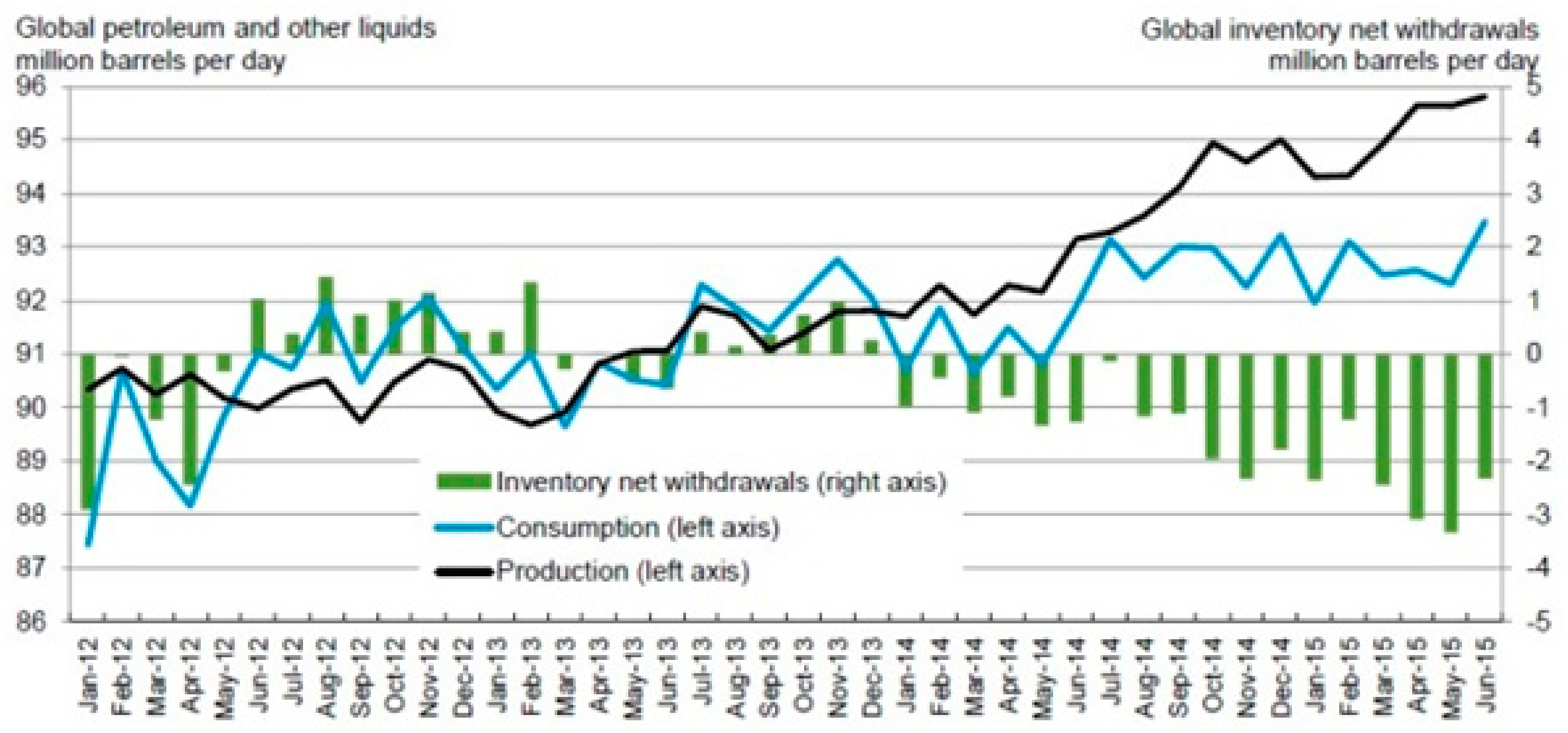
It is difficult to determine the direction and intensity of energy prices in the future. For example, the U.S. Energy Information Administration in its “Independent Statistics & Analysis” publication, “The Availability and Price of Petroleum and Petroleum Products Produced in Countries other than Iran” in its May–June 2015 update states the following:

“The uncertainty on both the supply and demand side of the market could result in large future price movements [underlined by the authors]. The possible lifting of sanctions on Iran could move additional supply on to the world market and reduce prices, while an unexpected supply disruption at a time of low surplus production capacity may push prices higher. Meanwhile, if a slowdown in global economic activity from current levels occurred, it would reduce demand and result in higher-than-expected inventory builds, moving prices lower” [42]. This can be seen from the graph from the same source in Figure 2, where the spread between production and consumption has been widening since July 2014.

In addition to the world energy price uncertainty, in Israel, there are at least four other sources for price uncertainty:

(a)

the possibility of military conflict;

(b)

the discovery of gas on Israel’s shore;

(c)

the adoption of gas by the industry; for example, Foenicia—a glass manufacturer that was recently close to bankruptcy due to lack of gas turned to become profitable [43]; and

(d)

the discovery of oil in the Golan Heights [44].

While it is still difficult with all these sources of uncertainty to determine the direction and intensity of the change of energy price, we must consider, thus, the possibility of high volatility in price. To this end, we will consider hereafter the possibility of high volatility taken to be StD = 40% per annum.

Calculating the call value based on the annual StD estimation of 0.4 yields 59.48 million $US (compared to 57.05 million $US based on StD of 0.031). It follows that the net profit of the first stage increased to 59.48 − 50 = 9.48 million $US (see Table 2, a column for the case of StD = 0.40). It would be worth noticing here that the main statistical parameters of the wind speed in the Merom Golan area, the mean and the StD, are observed with a tendency towards stability, without any significant divergence over the period of the last few years, 2009–2014, as it follows from the calculated data in

Table 3. Wind speed mean and StD at Merom Golan for the last period.

Year	2009	2010	2011	2012	2013	2014
Speed mean (m/s)	3.89	3.69	3.63	3.70	3.80	3.62
StD (m/s)	2.10	2.12	2.00	2.03	2.05	1.99
Number of Samples	2919	2920	2920	9774	2896	2898
StD/$\sqrt{n}$ (m/s)	0.039	0.039	0.037	0.021	0.038	0.037

:

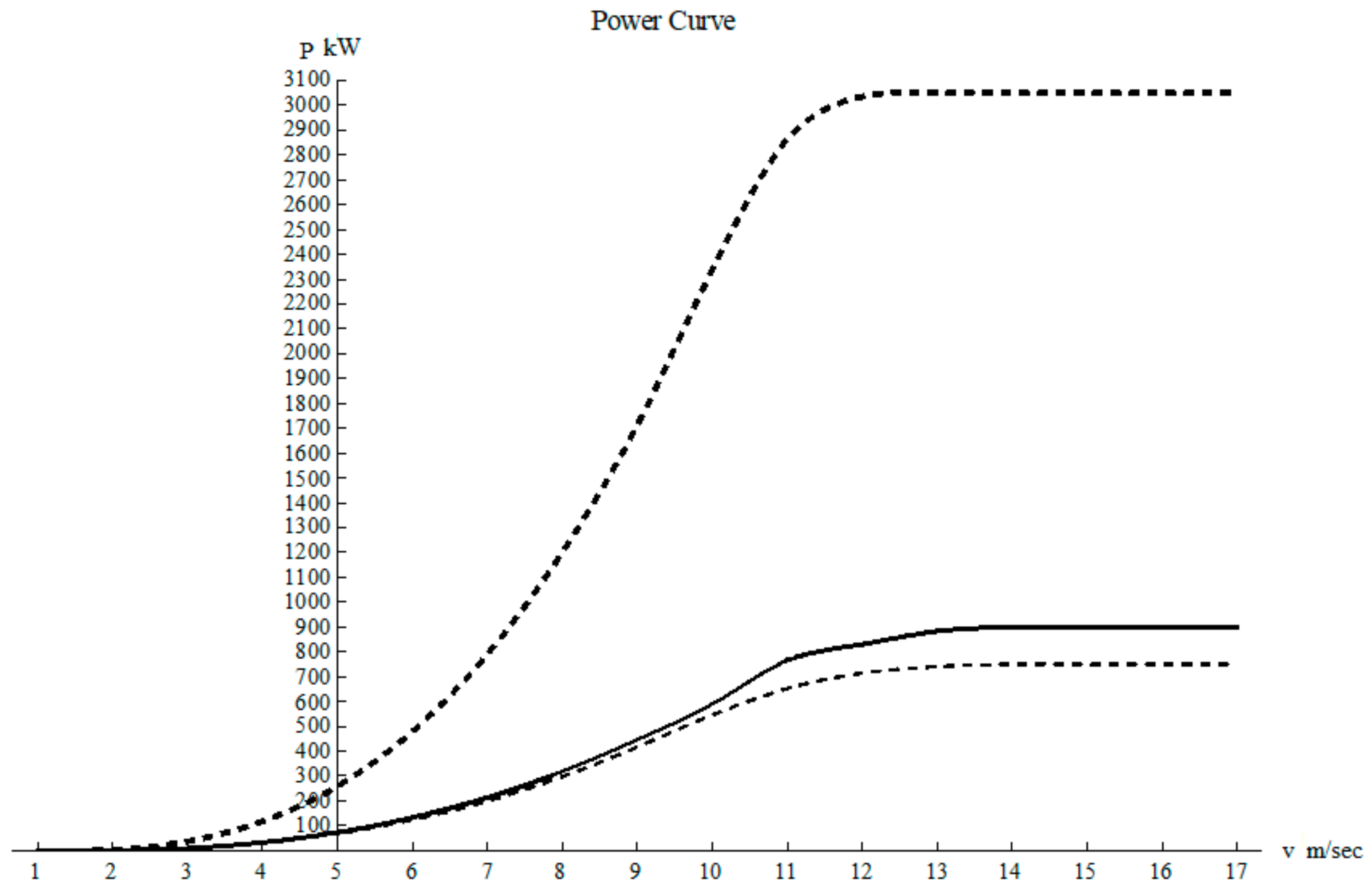
The expectation value of an annual average is the same as the expectation value for one sample, but the standard deviation of the annual average is equal to the standard deviation of one sample divided by the square root of the annual number of samples (see Appendix A for a mathematical justification). Thus, the standard deviation of the annual average of wind speed is between 0.6–1.1%, and can be further reduced by more sampling. A six year average based on 24,327 samples will be 3.72 m/s, with only 0.4% standard deviation. The power curves of available turbines are described in [45], from which three examples are analyzed in this paper and are depicted in Figure 3.

The wind speeds described in Table 3 are for a height of 10 m, for different heights, we apply the velocity to height connection [46]:

$$v\left(h\right)=v_{10 }{\left(\frac{h}{10}\right)}^a$$

in which $v\left(h\right)$ is the velocity at height h, $v_{10}$ is the velocity at a height of 10 m, and a is Hellmann’s exponent, which, for a neutral air above human inhabited areas, is about 0.34. Among the turbines analyzed, the largest is Enercon’s model E101/3000 turbine with a radius of 50.5 m. Hence, we will assume from now on that the hub of the turbine is 60 m.

Table 4. Wind turbine geometric parameters.

Turbine	Enercon’s E101/3000	AWE’s 54–900	EWT’s Directwind 52/750
Area (m2)	8012	2290	2083
Radius (m)	50.5	27	25.75

will summarize the area and radii of the turbines under study:

For this height, we obtain a six year speed average of 6.84 m/s. The eleven year average of the power and the standard deviation obtained for each turbine are depicted in

Table 5. Wind turbine power for eleven years of data acquisition.

Turbine	Enercon’s E101/3000	AWE’s 54–900	EWT’s Directwind 52/750
Average Power (kW)	1205.84	325.84	289.70
Power StD (kW)	1125.94	309.10	264.99
Power StD/$\sqrt{n}$ (kW)	6.36	1.75	1.50
%(StD/$\sqrt{n})$/Average	0.52	0.54	0.52
Annual Revenue (SH)	5,133,695	1,387,218	1,233,357
Annual Revenue ($)	1,327,909	358,825	319,027

, the total number of samples in this analysis was 31,292 based on the wind data from Merom Golan.

The standard deviation of average power for all turbines investigated is much lower than the standard deviations of energy price appearing in Table 2. Hence, a long-term project can ignore the risks connected with the standard deviation of wind speed. A formal proof for this decisive circumstance is given in Appendix B.

This circumstance determines the fact of non-relevancy of the speed variance over a prolonged period of time for the wind turbine economic value; this should be compared to the significance of the energy prices for the turbine economic value.

Table 5 also contains the annual economic value of the turbine based on the current price of energy for consumers in Israel, which is 0.486 SH for kW hour on 11 September, 2015, the exchange rate for the same date is 3.866 SH for one US$. We assume that the turbine owner will need to pay for transmission and distribution, hence the more conservative estimate of an annual profit of 0.2 million $US per turbine quoted in the previous section. In practice, the price is determined by governmental authorities who strike a balance between the interest of other producers, the cost of transmission and distribution, and the public interest in clean energy.

We previously concluded that the advantage of using ROA over DCF is most significant when the market prices are volatile, and less so when the energy prices are stable. However, the change in wind speed is a small fraction of the value of the wind installation volatility, and this alone cannot justify the use of the ROA method. However, the fluctuations of the market energy prices is reason enough.

5. Conclusions

Traditional calculation for an uncertain cash flow applies just to the expected values of the cash flow from the project without the possibility of abandoning the project. Given our empirical assumptions, this yields a loss of 1.3 million $US instead of profit, meaning the project becomes not worthwhile.

Nevertheless, applying the real option analysis, which reveals the value of the option to abandon the second stage running as well, we turn the project to just become profitable and worthwhile. The value of the real option increases depending on the volatility to be either 57.05 million $US or 59.50 million $US, depending on future volatility, and the profit is either 7.05 million $US or 9.48 million $US, respectively.

Finally, for civil engineering projects with volatility in input and mainly in output prices, it is important to consider the option to abandon the project from the beginning, as this option may turn the project to be profitable.

We underline that, for wind installations, the main volatility is due to energy market prices and less because of wind speed uncertainties, which average out on an annual time scale.

To conclude, we underline that our work contains the following innovative elements, which were not published before:

• Weibull statistics of the wind in Merom Golan based on data gathered for several years was obtained, thus deriving the relevant parameters needed for our work.
• Using the empiric wind data and power curves of commercial wind turbines to choose the best wind turbine for the Merom Golan site.
• Using the above data, we calculated the revenue from Merom Golan due to electric energy production.
• It was shown that, taking into account the annual energy production, fluctuations are rather small; this is contrasted with rather large fluctuations when one considers the data over a daily basis.
• This was integrated into two economic models; one is the standard discounted cash flow and the other is the real options analysis. We have shown that, because of energy price volatility and despite small technical fluctuations, the correct estimation of the investment is given by the real options analysis, which takes into account the ability of the investors to abort their investment after the first stage.

We thus make the following policy recommendation, which is particularly relevant in the current era of high energy price fluctuations (for example on 15 April 2020, the US WTI Crude was 19.87 US$, today (20 February 2021) it is 59.24 $. This is more than 40% difference, which is discussed in the current work). We recommend investors and policy makers to use real options analysis rather than standard discounted cash flow, and take advantage of the ability to abort an unprofitable endeavor.

Future directions in this research area include the analysis of real economic parameters that are not just rough estimates, and the use of more accurate analysis using approaches such as the binomial lattice, the mean reverting jump-diffusion method, and the stochastic volatility model.