Article

Few-Shot Learning with a Novel Voronoi Tessellation-Based Image Augmentation Method for Facial Palsy Detection

by
Olusola Oluwakemi Abayomi-Alli
1,
Robertas Damaševičius
1,*,
Rytis Maskeliūnas
2,3 and
Sanjay Misra
4,5
1
Department of Software Engineering, Kaunas University of Technology, 51368 Kaunas, Lithuania
2
Department of Applied Informatics, Vytautas Magnus University, 44404 Kaunas, Lithuania
3
Faculty of Applied Mathematics, Silesian University of Technology, 44-100 Gliwice, Poland
4
Department of Electrical and Information Engineering, Covenant University, Ota, Ogun State 112212, Nigeria
5
Department of Computer Engineering, Atilim University, 06830 Ankara, Turkey
*
Author to whom correspondence should be addressed.
Electronics 2021, 10(8), 978; https://doi.org/10.3390/electronics10080978
Submission received: 6 March 2021 / Revised: 13 April 2021 / Accepted: 16 April 2021 / Published: 19 April 2021
(This article belongs to the Section Bioelectronics)

Abstract

:
Face palsy has adverse effects on the appearance of a person and has negative social and functional consequences on the patient. Deep learning methods can improve face palsy detection rate, but their efficiency is limited by insufficient data, class imbalance, and high misclassification rate. To alleviate the lack of data and improve the performance of deep learning models for palsy face detection, data augmentation methods can be used. In this paper, we propose a novel Voronoi decomposition-based random region erasing (VDRRE) image augmentation method consisting of partitioning images into randomly defined Voronoi cells as an alternative to rectangular based random erasing method. The proposed method augments the image dataset with new images, which are used to train the deep neural network. We achieved an accuracy of 99.34% using two-shot learning with VDRRE augmentation on palsy faces from Youtube Face Palsy (YFP) dataset, while normal faces are taken from Caltech Face Database. Our model shows an improvement over state-of-the-art methods in the detection of facial palsy from a small dataset of face images.

1. Introduction

Facial palsy, commonly referred to as Bell’s palsy, is a major kind of facial nerve paralysis that leads to the loss of control of muscles in the affected facial areas [1]. Some of the symptoms include the deformity of the face and dysfunction of facial expressions on the affected side of the face. The impact of the disease in face palsy-affected patients could lead to serious disruption to their everyday living. The progress of the disease often leads to associated physical, psychological, and social disorders as the ability of the person to express his/her emotions and effectively communicate is hindered, leading to reduced quality of life, depression, and social stigmatization [2]. Currently, the detection of facial palsy depends solely on expert clinicians by performing a visual examination of facial symmetry and evaluation of facial expression dysfunction. The major challenge in the diagnosis of facial palsy is the lack of successful measures targeted towards the effective evaluation of facial nerve function, as it could play a crucial role in understanding the advancement of the disease [3].
In recent years, several computer vision-based methods for diagnosis and automated recognition of facial palsy have been proposed, while most methods utilized handcrafted features and classifiers [4]. A study in [5] introduced the electronic facial paralysis assessment tool, while the authors of [6] applied facial motion analysis to evaluate not just Bell’s palsy patients, but also synkinesis (involuntary contraction of muscles). Authors in [7] proposed multi-resolution local binary patterns (LBPs) to identify the local and global region patterns of facial palsy. The symmetry of facial movements was assessed using resistor-average distance (RAD) between the facial features. Support vector machine (SVM) was used for measuring evaluating facial palsy symptoms. A dataset of 197 videos was used, on which their proposed model achieved 94% accuracy. Authors in [8] presented an active shape model (ASM) for the detection of facial landmarks on patient’s faces. The faces were fragmented into eight regions and facial asymmetry was evaluated based on the separations between points of interest inside each locale and over comparing regions. SVM with radial basis function (RBF) kernel was used to predict the face palsy degrees using a database of images from 62 patients.
Authors in [9] proposed using the limited-orientation modified circular Gabor filters (LO-MCGFs) on face images of 75 facial palsy patients and 10 normal subjects. The proposed method was applied for noise removal and enhancing desired spatial frequencies. Besides, the authors integrated bounded filter support to identify the region of interest (ROI). The authors of [10] presented a smartphone-based diagnostics system, which applied an increasing face alignment for recognition of facial landmarks and calculation of face asymmetry index. The authors used linear discriminant analysis (LDA) and SVM classifiers on a face palsy dataset obtained from 23 face palsy subjects and 13 normal subjects. A similar study was presented by [11] that applied laser speckle contrast imaging to register facial blood flow images of FP patients. Facial blood image and RGB color image are used to extract 68 facial landmarks and reconstruct the 3D model of a face, which is used to train k-nearest neighbor (K-NN), SVM, and neural network (NN) classifiers, and accomplished an accuracy of 97.14% on a dataset of 8000 images. However, the drawback is their strong dependence on prior expert knowledge, which resulted in limitations in the accuracy of the classifier.
The increasing ability of deep learning-based methods to automatically learning discriminative features has helped to improve the overall performance of classifiers. Authors in [12] introduced a deep hierarchical network (DHN) using state-of-the-art YOLO-v3 [13] architecture for facial palsy detection. A further study by [14] used a deep convolutional neural network (CNN) for feature extraction and adopted a prediction model based on unilateral peripheral facial paralysis evaluation. A similar study by authors in [15] adopted a deep network to acquire palsy-specific features from face images, and a generative adversarial network (GAN) was used for creating a synthetic training dataset. A further study [16] used a multi-task CNN framework for concurrent facial detection and facial symmetry analysis. The authors in [17] applied a cascaded encoder strategy based on a dual-encoder structure to improve recognition of the facial semantic features for the prediction of grading facial paralysis. Finally, a study [18] suggested 3DPalsyNet, a 3D CNN architecture built upon the ResNet backbone, for the recognition of mouth motions during some dynamic tasks, which allows for performing facial palsy stage grading.
Research findings from discussed recent studies using the state-of-the-art-methods for automatic detection of a facial palsy show that facial asymmetry is the major factor in the detection of facial palsy [19], which underscores the importance of facial symmetry/asymmetry and facial beauty studies [15,20]. Another problem related to facial palsy detection is the lack of a large face image dataset required for training (or retraining) through transfer learning [21] modern complex deep network models such as VGG-16 [22] or ResNet [23]. For example, the dataset used in [24] has only 1049 clinical images, while the YouTube Facial Palsy (YFP) dataset [12] has videos from 21 subjects, which makes the training of deep networks while avoiding overfitting a difficult task.
The application of data augmentation methods has been successfully applied in face recognition systems to improve the performance of training models and overall learning results [25]. Data augmentation increases variation in the dataset in the case of small and insufficient data [26] and addresses the challenges related to the collection of more data such as patients’ privacy issues and so on. One of the most widely used approaches is the application of geometric and color transformation methods to create an augmented dataset of images [27]. Examples of the transformation method include affine transformations, blurring, brightness shift, channel shuffle, contrast shift, elastic transformations, image blending, reflection, rotation, and scaling [28]. The approaches based on data disruption are based on increasing the number of images in the dataset by generating images with reduced informational content. The examples include random cropping and random erasing [29]. These methods can improve the generalization ability of the network, thereby preventing it from overfitting. Changing the brightness, contrast, saturation, and noise in an image entails photometric distortion of images. Random scaling, cropping, flipping, and rotating are used in geometric distortion of images. Random erase, cutout, hide and seek, grid mask, and mixup image transforms are part of image occlusion. Random erase [29] is an augmentation technique that substitutes random values for regions of the image or the mean pixel value of the training set. It is usually applied with a varying percentage of the erased image and the erased field aspect ratio. It keeps the model from memorizing and overfitting the training data. Square regions are masked during training in cutout augmentation [30]. Only the first layer of the neural network hides cutout regions. This augmentation technique is similar to random erase, but in overlaid occlusion, with a constant value. In meshcut [31], a mesh mask transforms an image into a mosaic made with several image parts. In hide and seek [32], we break the picture into a patch grid and then conceal each patch with a certain probability. In cutmix [33], the image patches are cut and pasted among training set images, while ground truth labels are also mixed in accordance with the area of patches. The regions of the picture are hidden in a grid fashion in the gridmask augmentation [34]. This forces the classifier to learn component portions of what makes up an individual entity, similar to hide and seek. In YOLOv4, the mosaic augmentation was introduced [35]. It incorporates four training images into one. This makes it possible for the model to learn how to classify objects on a smaller than average scale. It also helps the model to locate various image types in various parts of the frame.
Another solution for small datasets is to apply the principles of one-shot learning [36] and a few shot-learning [37]. The idea capitalizes on transfer learning, while a network is retrained to solving new tasks containing only a few (or one, in an extreme case) samples with supervised information. Such an approach has been successfully applied in face recognition and identification systems before [38]. Few-shot learning methods can be classified into three types: metric-based learning, meta-learning, and fine tuning. Metric-learning approaches [39] address few-shot classification tasks by training an embedding function for the feature space. Meta-learning methods [40,41] tackle the few-shot learning problem by training neural networks to learn novel classes. Fine-tuning methods improve the performance of the neural network by updating its weights. In this paper, however, we use the data augmentation approach to few learning.
Based on the limitations of the existing methods for face palsy recognition and identified knowledge gaps, this paper presents the following contributions:
  • A new method for face palsy recognition based on the principles of data augmentation and few-shot (one-shot and two-shot) learning;
  • A novel image augmentation method, called Voronoi decomposition-based random region erasing (VDRRE), for generating new artificial images with randomly covered regions of irregular shape and augmenting the original dataset for more efficient neural network training;
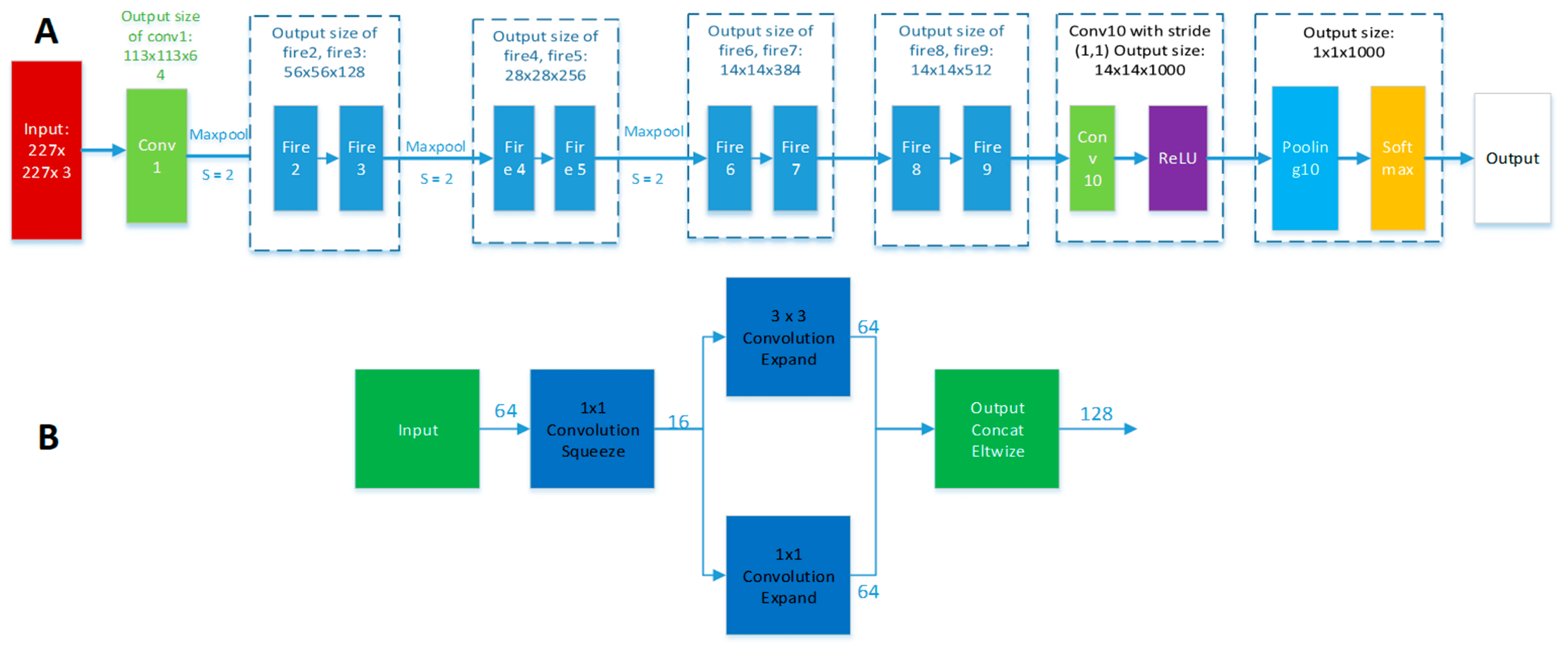
  • A hybrid face palsy detector that combines the pre-trained SqueezeNet network [42] as feature extractor and error-correcting output codes (ECOC)-based SVM (ECOC-SVM) as a classifier.
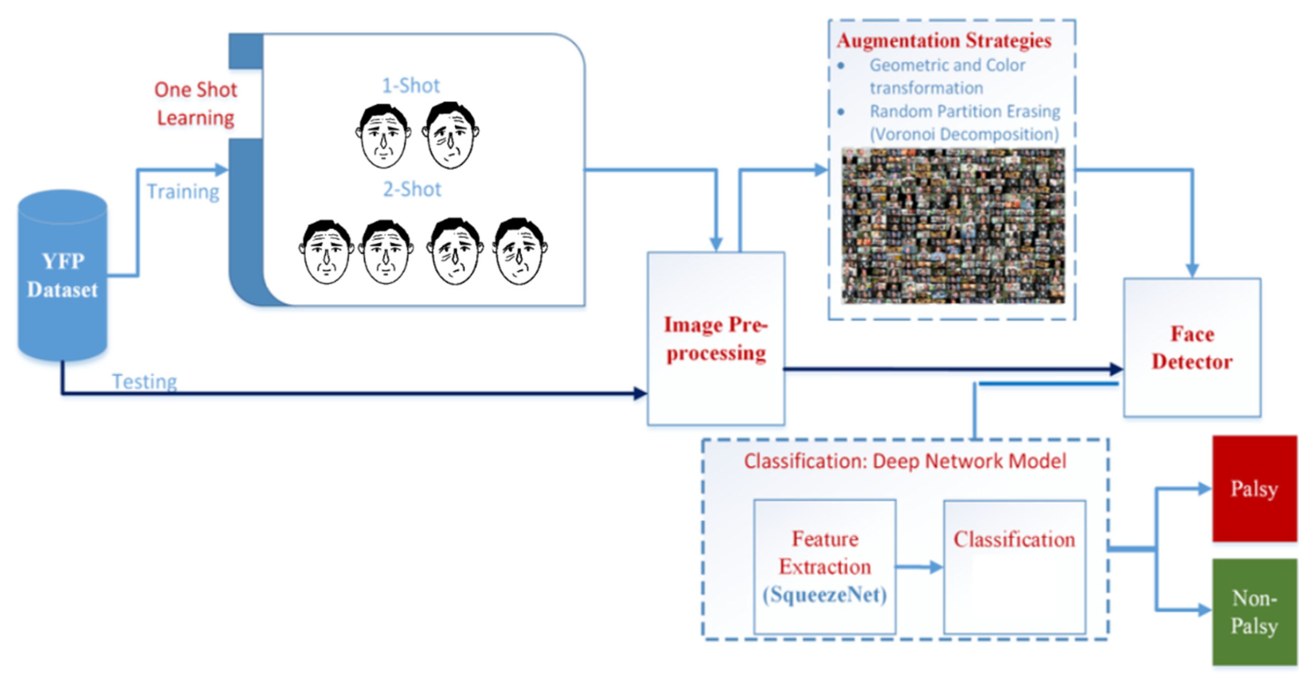
Other parts of this paper are outlined as follows. Section 2 describes the methodology and techniques used in this paper. The experimental results are discussed and a comparison with state-of-the-art-methods is presented in Section 3. Finally, Section 4 presents conclusions and future recommendations.

2. Methods

For the study, we focus on detecting face palsy from a very small number of training instances available for a deep network, thereby adopting the one-shot learning approach. The outline of the methodology is presented in Figure 1 and is divided into five stages, as highlighted below. A further explanation of all the processes involved is discussed in other subsections.
  • Data collection: The first stage is the original face image dataset consisting of 1555 data samples (1105 of palsy face dataset and 450 of normal face dataset).
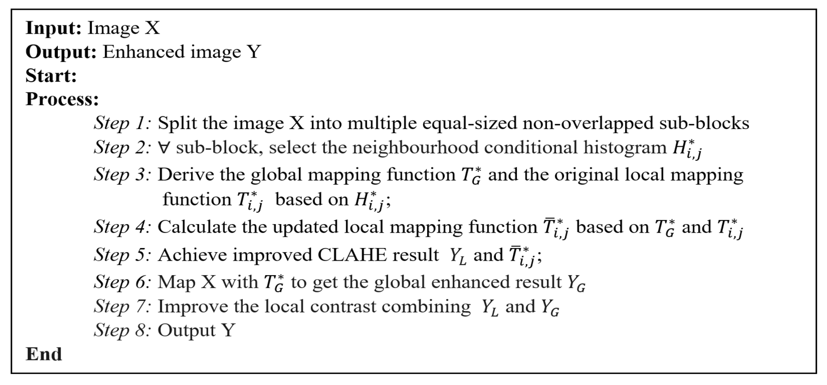
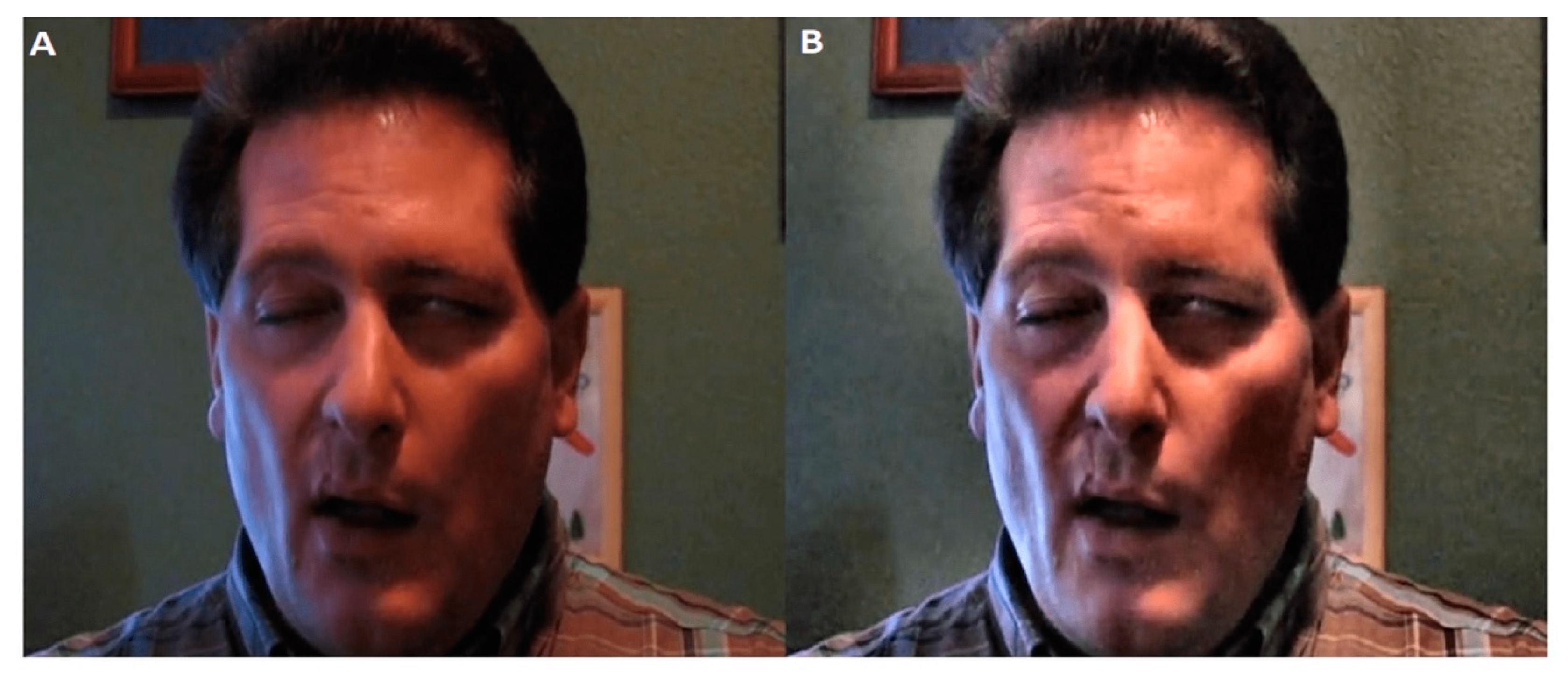
  • Data preprocessing: This stage includes the removal of noise and improvement of image contrast using contrast limited adaptive histogram equalization (CLAHE).
  • Few-shot learning: This stage tries to mimic human intelligence using only a few samples (one or two images, for each class) for supervised training.
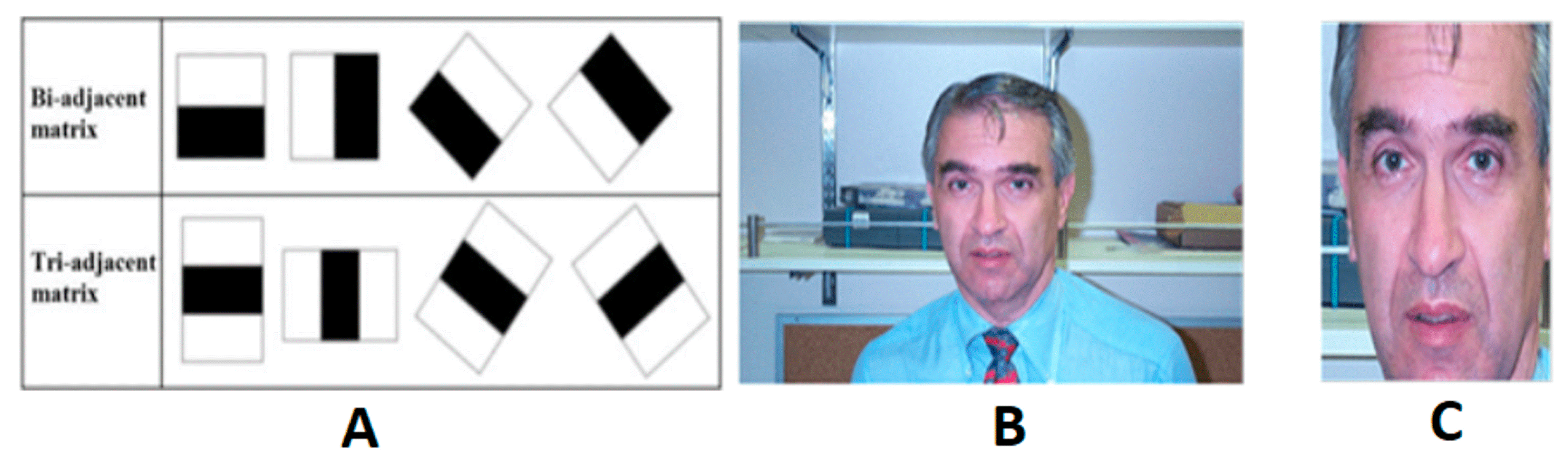
  • Face detector: We adopted the improved classical Viola–Jones face detection algorithm, which depends on the Haar-like rectangle feature expansion [43].
  • Augmentation strategy stage: we use the proposed Voronoi decomposition-based random region erasing (VDRRE) image augmentation method as well as adopted other data augmentation techniques to improve neural network training and generalization and solve class imbalance, thus addressing the problem of overfitting.
  • Classification: We adopted the SqueezeNet architecture, which has comparatively low computational demands, for feature extraction and ECOC-SVM as a classifier.

2.1. Dataset

The dataset used in our study is the YouTube Facial Palsy (YPF) dataset [12]. The YFP data consist of 32 videos of 21 patients gathered from YouTube and annotated by medical specialists. From the YFP dataset, we used 1105 palsy face images, which were already extracted from the YouTube videos by the authors of the dataset and presented as image sequences with a rate of 6 fps. All face images are frontal images with a unique shot under different lighting conditions, facial expressions, and cluttered backgrounds. The faces in these images have a resolution of 227 × 227 pixels.
The normal images were taken from Caltech Face [44] Database, which contains 450 face images of 27 unique people under different lighting/expressions/backgrounds. The size of these images has a resolution of 896 × 592 pixels, which were resized to 227 × 227 pixels to match the resolution of the faces in the YFP dataset. Therefore, the full dataset consists of 1555 facial images, which includes 1105 palsy images and 450 normal (non-palsy) images. An example of face palsy images is given in Figure 2.

2.2. Few-Shot Learning

Few-shot learning (FSL) is a learning from few or single training items [37]. The motivation for this model is based on the unique intelligence in humans with the ability to effectively generalize after only seeing a single example of a specific object. Thus, in this study, we have integrated the FSL approach to learning information about image features from a small number (one or two) of labeled image samples for each of the classes.
Few-shot learning concerns the practice of providing a learning model only with a very small amount of data for training, which is contrary to the common practice of using a very large amount of data. Formally, the few-shot approach trains a classifier h , which predicts label y i for input x i . Commonly, one considers the N -way- K -shot learning, in which the training dataset has K N samples from N classes each with K instances. Few-shot learning trains a classifier h given only a few input–output sample pairs, where output y i is the class (label) of the independent variable x i . An extreme case of few-shot learning is one-shot learning (OSL) [38], in which there is only one instance with class label available for the training of the classifier.
In few-shot classification, the goal is to reduce prediction error on unlabeled data. Let dataset d D contain pairs of features and labels { ( x i ,   y i ) } , where each label belongs to a known set of labels . Dataset d is divided into two parts: d = S ,   B , consisting of training S and testing B   samples. We accept a N-class K-shot problem, where the training set contains K labelled examples for each of the N classes. To implement it, we do the following:
  • Take a subset of labels, T ⊂   .
  • Take a training set S T D and a training set B T D . Both contain only data with labels from the subset from item 1: L ,   y L ,     ( x ,   y )   S T ,   B T .
  • The set of S T is fed to the input of the classifier model.
The final optimization uses many training sets B T to compute the loss function and update the model parameters through backpropagation, just like in the case of supervised learning.

2.3. Image Pre-Processing

For image pre-processing, we ensured that all the images were well aligned using the face detection method described in Section 2.4. We converted all colored face images into grayscale to eliminate unwanted color cast using contrast limited adaptive histogram equalization (CLAHE). CLAHE [45] was used to clip the histogram at a predefined value and limiting contrast amplification, and thus eliminating shadows, light variations, and removing noise. This study further applied an improved CLAHE method that replaces the clip-redistributed histogram with the so-called neighborhood conditional histogram [46]. Using this method, we have optimized the local contrast and enhanced the face images based on the edge information as presented by the algorithm in Figure 3.
The typical results of applying histogram equalization for the normalization of image contrast are shown in Figure 4.

2.4. Face Detection

We performed detection of the human faces in a specific image intending to identify and segment the human face from the background. Here, we adopted the improved Viola–Jones face detection method, which depends on the Haar-like rectangular feature expansion [43]. This detection algorithm integrated 2D convolution separation and image re-sampling techniques [47]. The classical Viola–Jones algorithm uses classifier boosting to merge shape and edge, template matching, and face feature models together. Initially, the Haar-like feature matrix is applied to scale facial features, and further feature evaluation is performed on the integral image. Instead of the orthogonal Haar-like rectangle features, the improved method uses a 45°-rotatable rectangle feature. The features were used for calculating the integral image value, and the pixel sum of all regions was obtained by image traversal. To effectively sample the face from the rest of the images, a cascade of weak classifiers was used. AdaBoost [48] was applied to develop stronger classifiers and to form a cascade classifier for removing non-face images and enhancing accuracy. This allows to eliminate of all redundant features and weak classifiers are cascaded to develop a powerful single classifier while window sliding over the entire image. An example of face detection using the 45°-rotated features is shown in Figure 5.

2.5. Data Augmentation

In this study, we considered image augmentation methods for generating artificial/synthetic data samples. The one-shot learning (OSL) samples for each class were augmented using the following image transform approaches: geometric transformation (rotation, cropping, reflection, translation, flipping), color transformation (histeq, enhanced histeq, adapthisteq, contrast adjustment, sharpening), and additionally noise was removed using blur filter, Gaussian filter, and edge-aware noise reduction.
For image augmentation, we have elaborated a random partition erasing image augmentation. The idea is based on random image cropping and patching proposed in [49] and random erasing proposed in [29], which used the rectangular blocks to occlude the image in random locations with noise (i.e., random pixel color values drawn from the uniform distribution). Here, we propose a novel image augmentation method, called Voronoi decomposition-based random region erasing (VDRRE). The method is based on a partition of a 2D plane into regions close to each of a given set of points. The coordinates of these points are generated using random numbers drawn from a uniform distribution as follows. First, we randomly select a number N of points in the image. Then, we create a partition, i.e., Voronoi tessellation [50], of an image into Voronoi regions close to each of a given set of objects as follows.
Assuming P = { p 1 ,   p 2 ,   ,   p n }   is a set of generators. For any region of X in the plane, d ( X , p n ) represents the distance from X to the generator point p n . For all possible locations of X in S , we set to the nearest generator p n P with a definite distance metric d . However, if it is close to two generators in P , then the distance becomes an edge; otherwise, if it is close to more than two generators, the location becomes a vertex. For any point p in the space, let d i s t ( p , X i )   denote the Euclidean distance from the point p to the primitive region X i . We can define the bisector of X i and X j by Equation (1) and the dominance region of X i over X j by Equation (2):
b ( X i , X j ) = { p | d i s t ( p , X i ) = d i s t ( p , X j ) } ,
D o m ( X i , X j ) = { p | d i s t ( p , X i ) d i s t ( p , X j ) } ,  
For a primitive X i , we can define the Voronoi region for X i as follows:
V ( X i ) =   j i D o m ( X i , X j ) ,
This set of points, V i ( S ) , is the Voronoi polygon associated with p i . Formally, V i ( S ) is described as follows:
V i ( S ) = { x   i n   R 2 |   d ( x ,   p i )     d ( x ,   q ) ;   a l l   q   i n   S } ,
This assignment results in an image decomposition, called Voronoi tessellation, that divides an image into several Voronoi cells bounded by image boundaries. Finally, a randomly selected Voronoi cell is filled with random pixel color values drawn from a uniform distribution to complete the occluding and produce a new image.
The method improves over the random erasing [29] method, as Voronoi tessellation generates more complex shapes of polygons beyond the simple rectangular shapes used. The method has only one hyperparameter to evaluate, i.e., the number of regions to erase as depicted in Figure 6 (the number of regions for partitioning is defined as six). Using this novel image augmentation method, we have created more images to enrich the training dataset based on different levels of occlusion, thus we were able to develop a more robust classification model while minimizing the possibility of overfitting.

2.6. Feature Extraction

Convolutional neural networks (CNNs) are commonly used to automatically extract discriminative features from images. Usually, pretrained neural networks such as AlexNet [51], VGG-16 [22], or ResNet [23] are used. A common approach is to remove fully connected layers from a pretrained network while retaining the remaining network, which has a series of convolution and pooling layers, as a fixed feature extractor [52]. Although, a recent study [53] has demonstrated that a shallow CNN constructed from just a few initial convolutional layers of a deep pretrained CNN can be very effective as well.
This study has applied a deep CNN to extract features from the YFP images. We adopted a lightweight pre-trained CNN, known as SqueezeNet [42], which has less than 1.5 million weights and performance close to AlexNet. The SqueezeNet architecture, depicted in Figure 7, was pre-trained on the ImageNet dataset [51], which has several millions of different images divided into 1000 classes.
We selected SqueezeNet over AlexNet and other alternatives (such as ResNet, VGG, Inception, and so on) because SqueezeNet has almost the same number of accumulated operations as AlexNet and could work with smaller file sizes of less 0.5 MB and with a smaller size of input images without any need for resizing, albeit the image size of 224 × 224 is still the ideal case. The main functional block of the SqueezeNet network is the fire unit, which is made of a squeeze layer (SL), expand layer (EL), and some pooling layers (PL). SL reduces the size of the feature map, while EL expands it again. To achieve a high level of abstraction, we increased the number of filters using the stride of two convolutional layers, and increased the depth and minimize the size of features. Our proposed solution can mitigate the problem of overfitting through transfer learning from a CNN pre-trained on an initially large generic dataset of images, rather than training it with random initial weights, as suggested in [54].

2.7. Classification

For classification, we adopted the multiclass, error-correcting output codes (ECOC)-based support vector machine (SVM) model (ECOC-SVM). The ECOC algorithm optimizes misclassification costs using class prior probabilities. This model creates K ( K 1 ) 2 binary SVM models using the 1-vs-1 coding design, where K is the count of unique class labels (for face palsy detection problem, the severity grade of palsy can be evaluated using five levels (grades) from I—mild to V—total paralysis [55]). The ECOC model can enhance overall performance when compared with other multiclass models [56]; however, if needed, it can be easily reduced to the binary classifier. We used SVM because it performs optimally in cases where there is a distinct margin of separation among classes. It has also been shown to perform well in highly dimensional data, particularly when the number of dimensions exceeds the sample size [57].

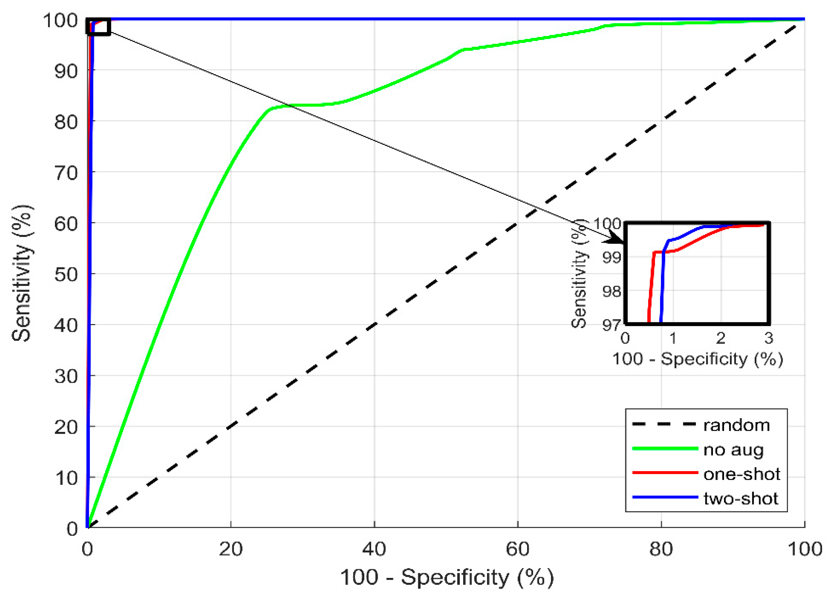
2.8. Performance Metrics

Considering class imbalance challenges with the dataset, evaluating just one metric such as accuracy might not be sufficient to investigate the overall performance of the model. We measure the performance of our model using four evaluation metrics: accuracy, precision, recall, and F1-score, which are expressed as follows:
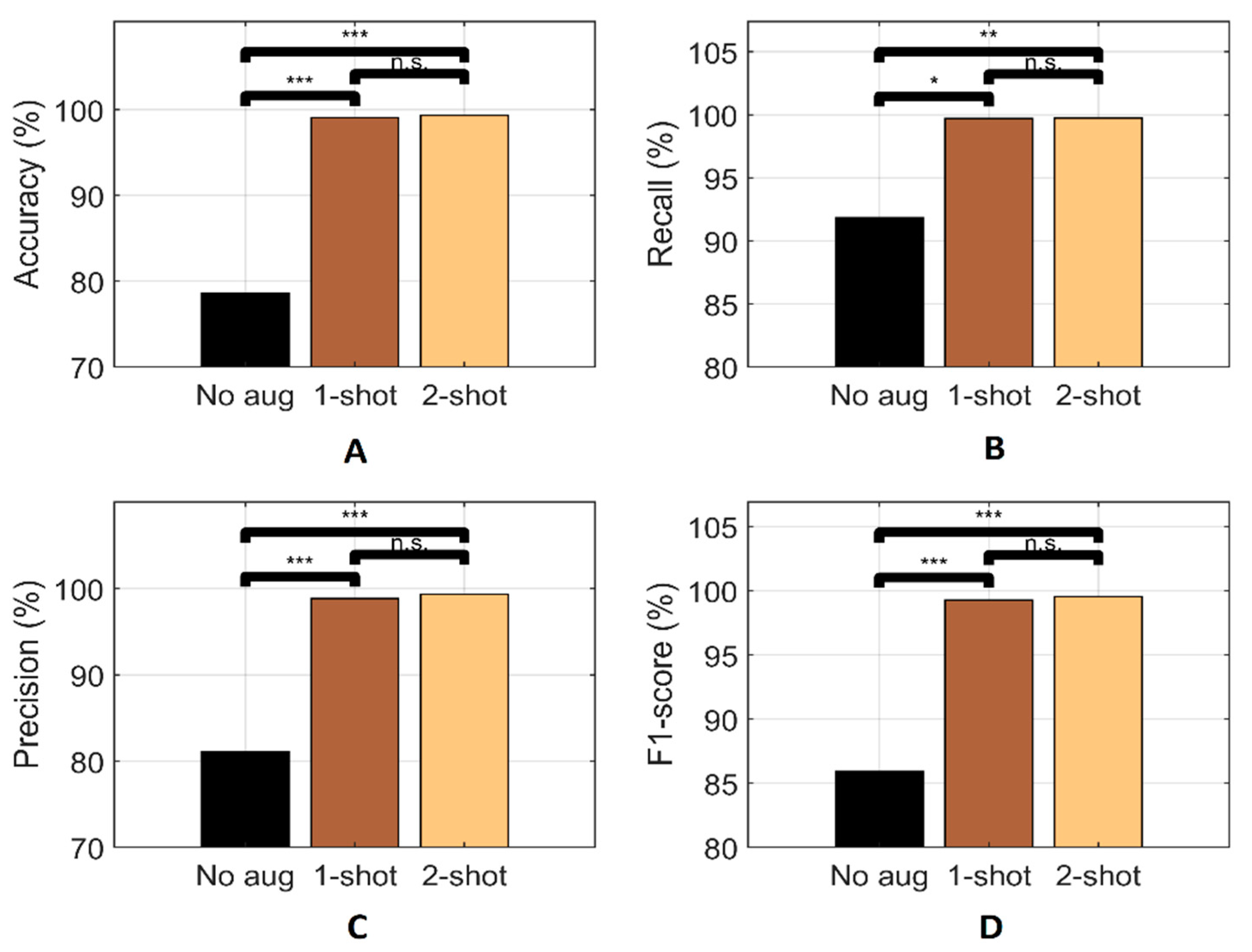
  • Accuracy is the measure of correctness of predicted classes:
    A c c u r a c y = 100 % ( T P + T N ) ( T P + T N + F P + F N ) ,
  • Precision is the proportion of predicted positive class that comes from the correctly real positive (palsy) class:
    P r e c i s i o n = 100 % T P ( T P + F P ) ,
  • Recall is the proportion of real positive class (palsy class) that are correctly predicted:
    R e c a l l = 100 % T P ( T P + F N ) ,  
  • F1-score is the weighted harmonic average of precision and recall:
    F 1 S c o r e = 2 P r e c i s i o n R e c a l l ( P r e c i s i o n + R e c a l l ) ,

2.9. Experimental Settings

The proposed method was implemented on MATLAB R2019a (Mathworks, USA) running on Windows 10 64 bits Intel Core i5 CPU and 8 GB RAM. First, the dataset images were processed using the improved CLAHE method to improve contrast and reduce noisiness. Then, the improved classical Viola–Jones face detection algorithm was applied to detect faces in the images. The accuracy of the feature detection stage was 100%, which was verified manually by checking each image. The high accuracy of face detection is explained as follows: each image in a dataset contains a single person with a frontal upright face in front of the camera, which makes the face detection task relatively easy. For further stages, we use the detected face segments in each segment to reduce the impact of the background on the training and classification results.
The experiments performed in this study are categorized into three scenarios; the first experiment was conducted using the original images from the YFP dataset, and the results were used as a baseline to compare against our proposed method. For the second experiment, we adopted the one-shot learning approach, and we randomly selected a single image for each class as a training sample. This one-shot sample data were augmented using the proposed VDRRE method to create 210 new samples for each class (a total of 420 images). The experiment was repeated 10 times, and the average of performance measures was calculated and used for evaluation. For the third experiment, we adopted the FSL approach. We randomly selected two images for each class as a training sample. These two-shot sample data were augmented using the proposed VDRRE image augmentation method to create 175 new samples for each class (a total of 700 images). The experiment was also repeated 10 times, and the average of performance measures was calculated and used for evaluation. The generated (one-shot and two-shot) images were used for training the SqueezeNet model, while images from the original dataset were used for testing. We ensured that there was no overlap between any of the datasets and testing was conducted on the original dataset only.
For training the SqueezeNet network, we used a learning rate of 0.00001, the stochastic gradient descent momentum (SGDM) optimizer, a fixed mini-batch of size 16, while the maximum set of epoch numbers was set to 50. For exponential decay rates, moment estimates, and epsilon parameters, we used the values of 0.9, 0.999, and 10–8 respectively. We used early stopping of training [58] to avoid overfitting. We stopped the training as soon as the validation loss began to rise, meaning that the generalization ability of the model started to decrease. The parameters of the trained model right before the validation loss starts to increase were saved and used for testing.
Finally, we used the activations from the final convolutional layer (which has 1000 weights) as features to train the ECOC-SVM classifier. Note that our methodology assumes that, in the general case, palsy images with palsy severity score can be used, thus we use the multiclass ECOC-SVM classifier. In this case, as we used the YFP dataset with binary labeled—‘normal’ and ‘palsy’—images, it is equivalent to a SVM classifier with a linear kernel.

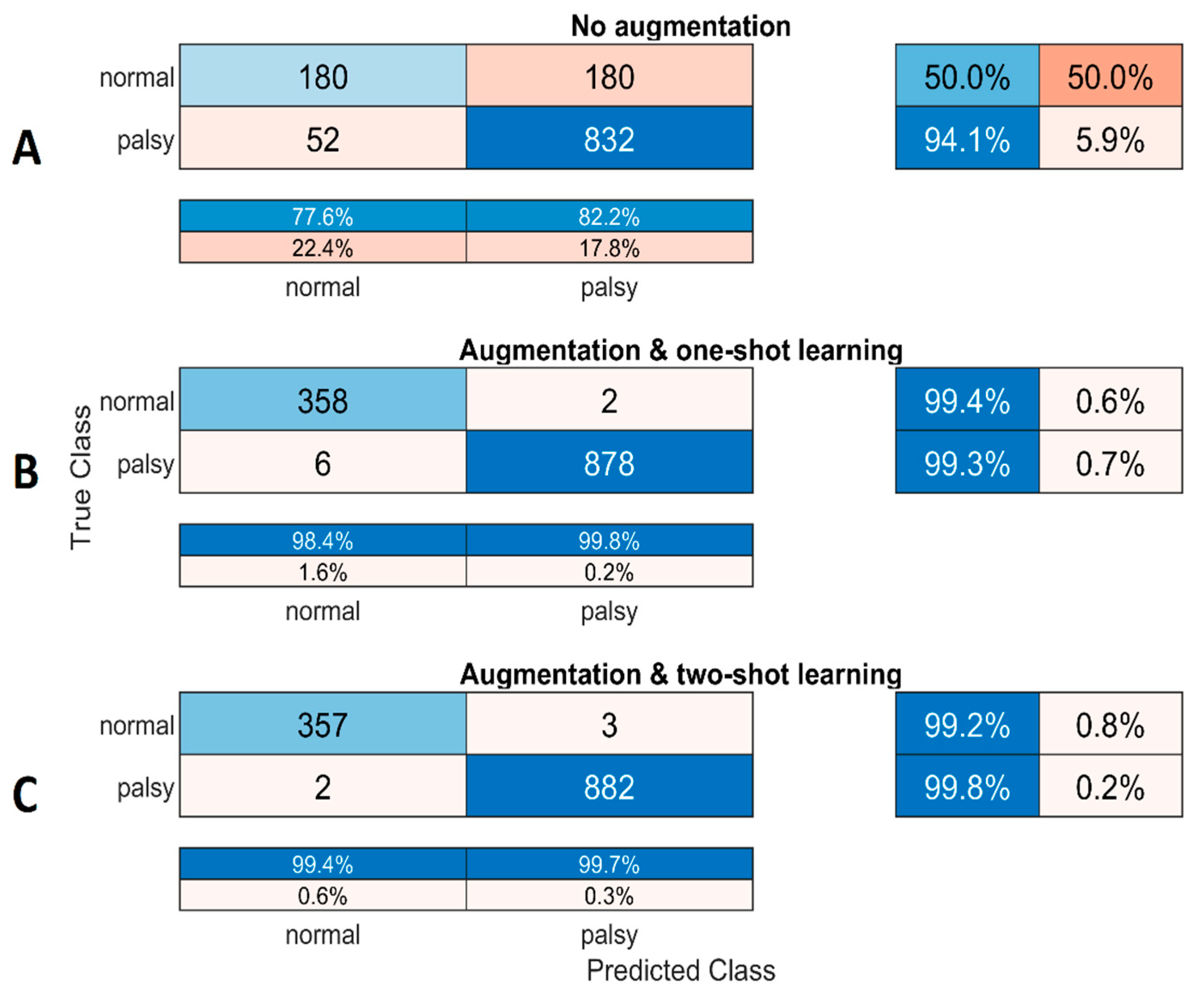
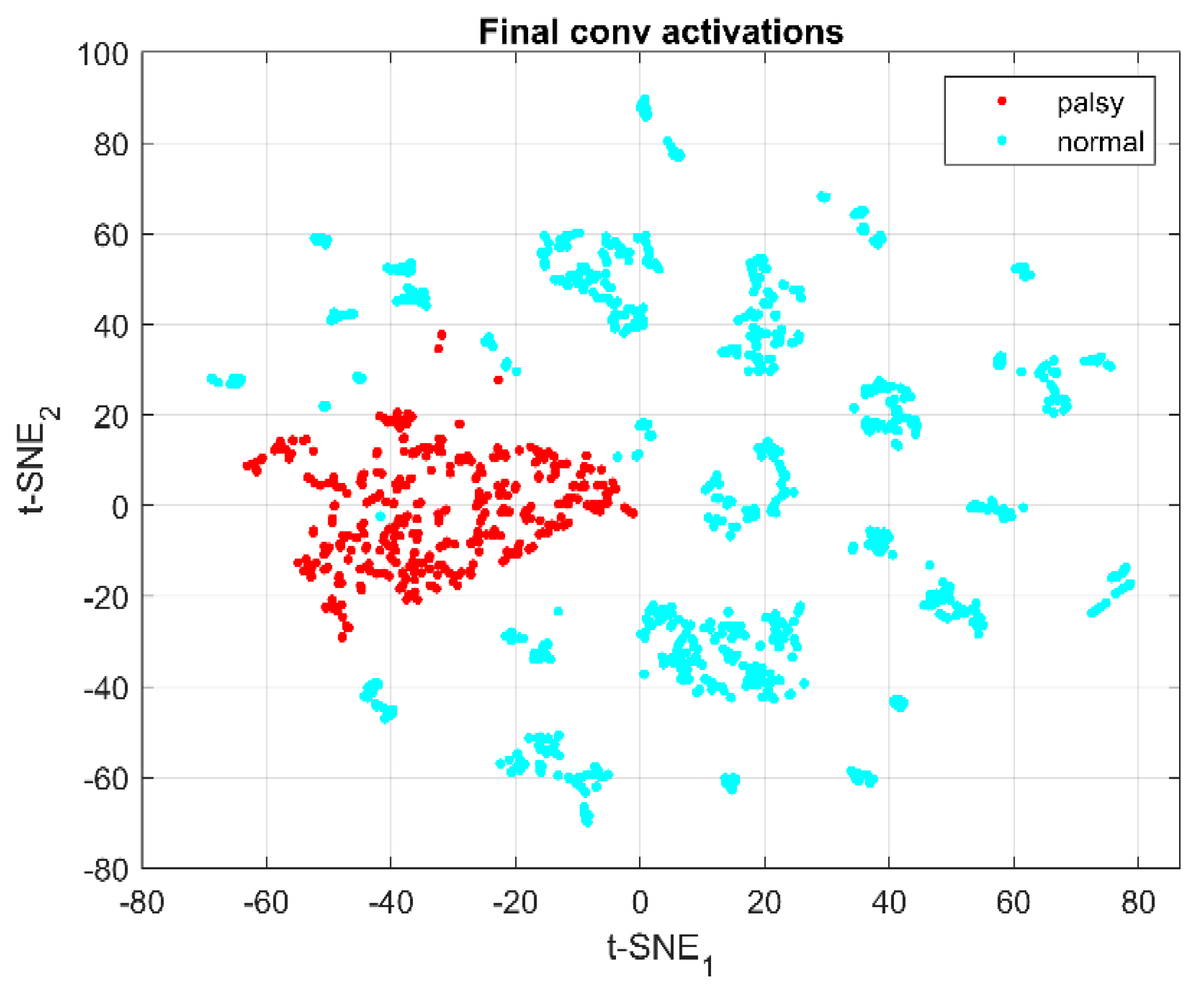
3. Experimental Results

As suggested by authors in [12] and for comparability, we split the dataset randomly into five subject-independent subsets, and performed five-fold cross-validation. Here, 80% of the dataset was used for training and 20% for testing. The experiments were repeated ten times each and we computed various performance (accuracy, recall, precision, and F1-score) metrics, which are reproduced in detail in Table 1, while the average values with 95% confidence limits are given in Table 2.
Figure 8 shows the confusion matrices for all three experiments. The confusion matrices show aggregated results from multiple cross-validation folds. Note that, for the one-shot and two-shot learning experiments with image augmentation, the rate of misclassification is low, which indicates good performance.
The best performance was obtained using two-shot learning with the proposed VDRRE method using the hybrid SqueezeNet/ECOC-SVM classifier, achieving 99.34% accuracy, 99.74% recall, 99.35% precision, and 99.54% F1-score. The results for the corresponding case with one-shot learning were only slightly worse, achieving 99.07% accuracy, 99.72% recall, 98.85% precision, and 99.28% F1-score. However, both one-shot and two-shot learning with VDRRE augmentation achieved much better results than the baseline (classification on original dataset images without any data augmentation), which achieved only 78.62% accuracy, 91.85% recall, 81.06% precision, and 85.59% F1-score.
To effectively visualize the ability of the SqueezeNet network to extract efficient features, we used the t-distributed stochastic neighbor embedding (t-SNE), which uses principal component analysis (PCA) for feature dimension reduction. t-SNE [59] is a nonlinear dimensionality decreasing method that allows for the visualization of high-dimensional data into a 2D map as shown in Figure 9. The results depicted in Figure 9 clearly show that the 2D embeddings of palsy face images make a cluster, which is well separated from the 2D embedding of normal face images.
To further compare models in three scenarios (original images without augmentation, one-shot learning with augmentation, and two-shot learning with augmentation), we used the receiver operating characteristic (ROC) curve, which is reproduced in Figure 10.
The ROC curves were used to calculate the area under curve (AUC) metric, which is equal to 0.7967 (95% CI = [0.7944, 0.7989]), 0.9958 (95% CI = [0.9957, 0.9959]), and 0.9956 (95% CI = [0.9955, 0.9957]), for original images with no augmentation as well as one-shot learning and two-shot learning scenarios, respectively. Here, the confidence intervals (CIs) were calculated by performing bootstrapping on the classifier performance matrix values while assuming their normal distribution. These results show that, in both the one-shot and two-shot scenario, the proposed VDRRE method allows to achieve significantly better performance over the “no augmentation” case.
For statistical analysis of the results, we used a two-sample t-test for equal means, which returns a decision on the null hypothesis that the data in both compared samples come from normal distributions with equal means, but unknown variances. The tests were performed at the 5% significance level. The results, presented in Figure 11, show that there is a significant (p < 0.001) difference between the one-shot learning scenario with VDRRE augmentation and the baseline (without any augmentation), as well as between the two-shot learning scenario with VDRRE augmentation and the baseline. However, the difference between the performance of the one-shot learning scenario and the two-shot learning scenario was not significant (i.e., equal means hypothesis is not rejected).

Comparison with Related Work and Discussion

To validate our results, we compared them with the experimental results of relevant studies using the same YFP dataset, as summarized in Table 3, which shows the results of current studies from [12,60]. The comparison shows that our results outperform the existing studies with a clear improvement in accuracy, precision, and recall. The improvement in the performance is due to the use of the proposed novel VDRRE image augmentation method, which allowed to increase the number of images available for neural network training.
Despite the good results achieved owing to the proposed image augmentation method, the following limitations of using a small dataset remain: (1) small datasets have smaller variability in representing the severity of the facial palsy disease; (2) the danger of overfitting (which results in a poor generalization of the deep network models) remains. However, from Figure 7, one can note that overfitting is not noticeable when image augmentation is applied as there is no large difference between training loss and validation loss. The validity of our results can be influenced by the binary setting of the experiment (i.e., normal vs. palsy), which does not discriminate between severity levels of facial palsy. This means that the variability within the ‘palsy’ class may be larger than between the ‘palsy’ and ‘normal’ classes. However, our methodology is generic and allows for using other facial palsy datasets with severity level class labels owing to the multiclass classifier ECOC-SVM used in the last stage of the workflow, which allows for seamless substitution of the datasets. In our future work, we will use the proposed methodology for the prediction of a palsy severity grade as well.

4. Conclusions

This paper introduced a classification workflow based on deep learning for facial palsy detection and classification. Our proposed methodology introduced a novel image augmentation method that extended the random erasing augmentation with irregular regions constructed using Voronoi tessellation. Then, we used an automatic deep feature extraction based on the SqueezeNet deep neural network, followed by the multi-class classifier at the final stage of the workflow. As a result, the proposed methodology can be applied for facial palsy assessment using various facial palsy datasets, including the multi-class ones, which have face images labeled with palsy severity grades.
To validate the efficiency of our model, we adopted the human intelligence-inspired model based on few-shot learning to train our system to recognize palsy face images from a few examples. We proposed the VDRRE image augmentation method for generating new training samples for one-shot and two-shot learning scenarios. We used our newly generated image datasets to train the proposed hybrid classifier and used the images from the original YFP and Caltech datasets to test. Our study showed the effectiveness of the proposed approach for facial palsy detection, achieving a statistically significant (p < 0.001) improvement over the performance of the baseline classification scenario as well as demonstrating a higher performance than the results of other authors achieved using the same YFP dataset.
The future recommendation is to explore other advanced data augmentation methods to generate synthetic datasets and develop a robust classifier with low computational complexity through combining transfer learning models for the early detection of face palsy with low severity grades. We also will explore the robustness of our method using different face palsy datasets and performing a cross-dataset validation of our proposed method.

Author Contributions

Conceptualization, R.D. and R.M.; methodology, R.D.; software, O.O.A.-A. and R.D.; validation, R.D., R.M., and S.M.; formal analysis, R.M. and S.M.; investigation, O.O.A.-A. and R.D.; writing—original draft preparation, O.O.A.-A., S.M., and R.D.; writing—review and editing, R.D. and R.M.; visualization, O.O.A.-A. and R.D.; supervision, R.D.; funding acquisition, R.D. All authors have read and agreed to the published version of the manuscript.

Funding

This research received no external funding.

Data Availability Statement

YFP dataset is available from https://sites.google.com/view/yfp-database (accessed on 12 April 2021). Caltech Face Database is available from http://www.vision.caltech.edu/archive.html (accessed on 12 April 2021).

Conflicts of Interest

There are no conflicts of interest.

References

  1. Gilden, D.H. Bell’s palsy. N. Engl. J. Med. 2004, 351, 1323–1331. [Google Scholar] [CrossRef] [Green Version]
  2. Nellis, J.C.; Ishii, M.; Byrne, P.J.; Boahene, K.; Dey, J.K.; Ishii, L.E. Association Among Facial Paralysis, Depression, and Quality of Life in Facial Plastic Surgery Patients. JAMA Facial Plast. Surg. 2017, 19, 190–196. [Google Scholar] [CrossRef] [Green Version]
  3. Lou, J.; Yu, H.; Wang, F. A review on automated facial nerve function assessment from visual face capture. IEEE Trans. Neural Syst. Rehabil. Eng. 2020, 28, 488–497. [Google Scholar] [CrossRef]
  4. Kihara, Y.; Duan, G.; Nishida, T.; Matsushiro, N.; Chen, Y.-W. A dynamic facial expression database for quantitative analysis of facial paralysis. In Proceedings of the 2011 6th International Conference on Computer Sciences and Convergence Information Technology (ICCIT), Seogwipo, Korea, 29 November–1 December 2011; pp. 949–952. [Google Scholar]
  5. Banks, C.A.; Bhama, P.K.; Park, J.; Hadlock, C.R.; Hadlock, T.A. Clinician-graded electronic facial paralysis assessment: The eFACE. Plast. Reconstr. Surg. 2015, 136, 223–230. [Google Scholar] [CrossRef]
  6. Linstrom, C.J. Objective facial motion analysis in patients with facial nerve dysfunction. Laryngoscope 2002, 112, 1129–1147. [Google Scholar] [CrossRef] [PubMed]
  7. He, S.; Soraghan, J.J.; O’Reilly, B.F.; Xing, D. Quantitative analysis of facial paralysis using local binary patterns in biomedical videos. IEEE Trans. Biomed. Eng. 2009, 56, 1864–1870. [Google Scholar] [CrossRef] [PubMed] [Green Version]
  8. Wang, T.; Dong, J.; Sun, X.; Zhang, S.; Wang, S. Automatic recognition of facial movement for paralyzed face. Bio-Med. Mater. Eng. 2014, 24, 2751–2760. [Google Scholar] [CrossRef] [Green Version]
  9. Ngo, T.H.; Seo, M.; Matsushiro, N.; Xiong, W.; Chen, Y.-W. Quantitative analysis of facial paralysis based on limited-orientation modified circular Gabor filters. In Proceedings of the 2016 23rd International Conference on Pattern Recognition (ICPR), Cancún, Mexico, 4–8 December 2016; pp. 349–354. [Google Scholar] [CrossRef]
  10. Kim, H.S.; Kim, S.Y.; Kim, Y.H.; Park, K.S. A smartphone-based automatic diagnosis system for facial nerve palsy. Sensors 2015, 15, 26756–26768. [Google Scholar] [CrossRef] [PubMed] [Green Version]
  11. Jiang, C.; Wu, J.; Zhong, W.; Wei, M.; Tong, J.; Yu, H.; Wang, L. Automatic facial paralysis assessment via computational image analysis. J. Healthc. Eng. 2020. [Google Scholar] [CrossRef]
  12. Hsu, G.J.; Kang, J.; Huang, W. Deep hierarchical network with line segment learning for quantitative analysis of facial palsy. IEEE Access 2019, 7, 4833–4842. [Google Scholar] [CrossRef]
  13. Redmon, J.; Farhadi, A. YOLOv3: An Incremental Improvement. arXiv 2018, arXiv:1804.02767. [Google Scholar]
  14. Guo, Z.; Dan, G.; Xiang, J. An unobtrusive computerized assessment framework for unilateral peripheral facial paralysis. IEEE J. Biomed. Health Inform. 2018, 22, 835–841. [Google Scholar] [CrossRef]
  15. Sajid, M.; Shafique, T.; Baig, M.J.A.; Riaz, I.; Amin, S.; Manzoor, S. Automatic grading of palsy using asymmetrical facial features: A study complemented by new solutions. Symmetry 2018, 10, 242. [Google Scholar] [CrossRef] [Green Version]
  16. Storey, G.; Jiang, R. Face symmetry analysis using a unified multi-task cnn for medical applications. In Proceedings of the SAI Intelligent Systems Conference, IntelliSys 2018: Intelligent Systems and Applications, London, UK, 5–6 September 2018; pp. 451–463. [Google Scholar] [CrossRef]
  17. Wang, T.; Zhang, S.; Liu, L.; Wu, G.; Dong, J. Automatic Facial Paralysis Evaluation Augmented by a Cascaded Encoder Network Structure. IEEE Access 2019, 7, 135621–135631. [Google Scholar] [CrossRef]
  18. Storey, G.; Jiang, R.; Keogh, S.; Bouridane, A.; Li, C. 3DPalsyNet: A facial palsy grading and motion recognition framework using fully 3D convolutional neural networks. IEEE Access 2019, 7, 121655–121664. [Google Scholar] [CrossRef]
  19. Kim, J.; Lee, H.R.; Jeong, J.H.; Lee, W.S. Features of facial asymmetry following incomplete recovery from facial paralysis. Yonsei Med. J. 2010, 51, 943–948. [Google Scholar] [CrossRef] [Green Version]
  20. Wei, W.; Ho, E.S.L.; McCay, K.D.; Damaševičius, R.; Maskeliūnas, R.; Esposito, A. Assessing facial symmetry and attractiveness using augmented reality. Pattern Anal. Appl. 2021. [Google Scholar] [CrossRef]
  21. Pan, S.J.; Yang, Q. A Survey on Transfer Learning. IEEE Trans. Knowl. Data Eng. 2010, 22, 1345–1359. [Google Scholar] [CrossRef]
  22. Simonyan, K.; Zisserman, A. Very deep convolutional networks for large-scale image recognition. arXiv 2014, arXiv:1409.1556. [Google Scholar]
  23. He, K.; Zhang, X.; Ren, S.; Sun, J. Deep Residual Learning for Image Recognition. In Proceedings of the 2016 IEEE Conference on Computer Vision and Pattern Recognition (CVPR), Las Vegas, NV, USA, 27–30 June 2016; pp. 770–778. [Google Scholar]
  24. Song, A.; Wu, Z.; Ding, X.; Hu, Q.; Di, X. Neurologist Standard Classification of Facial Nerve Paralysis with Deep Neural Networks. Future Internet 2018, 10, 111. [Google Scholar] [CrossRef] [Green Version]
  25. Wang, X.; Wang, K.; Lian, S. A survey on face data augmentation for the training of deep neural networks. Neural Comput. Appl. 2020, 32, 15503–15531. [Google Scholar] [CrossRef] [Green Version]
  26. Kitchin, R.; Lauriault, T.P. Small data in the era of big data. GeoJournal 2015, 80, 463–475. [Google Scholar] [CrossRef]
  27. Porcu, S.; Floris, A.; Atzori, L. Evaluation of Data Augmentation Techniques for Facial Expression Recognition Systems. Electronics 2020, 9, 1892. [Google Scholar] [CrossRef]
  28. Buslaev, A.; Iglovikov, V.I.; Khvedchenya, E.; Parinov, A.; Druzhinin, M.; Kalinin, A.A. Albumentations: Fast and Flexible Image Augmentations. Information 2020, 11, 125. [Google Scholar] [CrossRef] [Green Version]
  29. Zhong, Z.; Zheng, L.; Kang, G.; Li, S.; Yang, Y. Random Erasing Data Augmentation. In Proceedings of the AAAI Conference on Artificial Intelligence (AAAI-20), New York, NY, USA, 7–12 February 2020. [Google Scholar]
  30. DeVries, T.; Taylor, G.W. Improved Regularization of Convolutional Neural Networks with Cutout. arXiv 2017, arXiv:1708.04552. [Google Scholar]
  31. Jiang, W.; Zhang, K.; Wang, N.; Yu, M. MeshCut data augmentation for deep learning in computer vision. PLoS ONE 2020, 15, e0243613. [Google Scholar] [CrossRef] [PubMed]
  32. Singh, K.K.; Yu, H.; Sarmasi, A.; Pradeep, G.; Lee, Y.J. Hide-and-Seek: A Data Augmentation Technique for Weakly-Supervised Localization and Beyond. arXiv 2018, arXiv:1811.02545. [Google Scholar]
  33. Yun, S.; Han, D.; Oh, S.J.; Chun, S.; Choe, J.; Yoo, Y. CutMix: Regularization Strategy to Train Strong Classifiers with Localizable Features. arXiv 2019, arXiv:1905.04899. [Google Scholar]
  34. Chen, P.; Liu, S.; Zhao, H.; Jia, J. GridMask Data Augmentation. ArXiv 2020, arXiv:2001.04086. CoRR abs/2001.04086. [Google Scholar]
  35. Bochkovskiy, A.; Wang, C.Y.; Liao, H.Y.M. YOLOv4: Optimal Speed and Accuracy of Object Detection. arXiv 2020, arXiv:2004.10934. [Google Scholar]
  36. Fei-Fei, L.; Fergus, R.; Perona, P. One-shot learning of object categories. IEEE Trans. Pattern Anal. Mach. Intell. 2006, 28, 594–611. [Google Scholar] [CrossRef] [PubMed] [Green Version]
  37. Wang, Y.; Yao, Q.; Kwok, J.T.; Ni, L.M. Generalizing from a Few Examples: A Survey on Few-shot Learning. ACM Comput. Surv. 2020, 53, 63. [Google Scholar] [CrossRef]
  38. O’Mahony, N.; Campbell, S.; Carvalho, A.; Krpalkova, L.; Hernandez, G.V.; Harapanahalli, S.; Riordan, D.; Walsh, J. One-Shot Learning for Custom Identification Tasks: A Review. Procedia Manuf. 2019, 38, 186–193. [Google Scholar] [CrossRef]
  39. Jiang, W.; Huang, K.; Geng, J.; Deng, X. Multi-Scale Metric Learning for Few-Shot Learning. IEEE Trans. Circuits Syst. Video Technol. 2021, 31, 1091–1102. [Google Scholar] [CrossRef]
  40. Gu, K.; Zhang, Y.; Qiao, J. Ensemble Meta-Learning for Few-Shot Soot Density Recognition. IEEE Trans. Ind. Inform. 2020, 17, 2261–2270. [Google Scholar] [CrossRef]
  41. Li, Y.; Yang, J. Meta-learning baselines and database for few-shot classification in agriculture. Comput. Electron. Agric. 2021, 182, 106055. [Google Scholar] [CrossRef]
  42. Iandola, F.N.; Han, S.; Moskewicz, M.W.; Ashraf, K.; Dally, W.J.; Keutzer, K. SqueezeNet: AlexNet-level accuracy with 50× fewer parameters and <0.5 MB model size. arXiv 2016, arXiv:1602.07360. [Google Scholar]
  43. Viola, P.; Jones, M. Rapid object detection using a boosted cascade of simple features. In Proceedings of the 2001 IEEE Computer Society Conference on Computer Vision and Pattern Recognition, Kauai, HI, USA, 8–14 December 2001. [Google Scholar] [CrossRef]
  44. Caltech Face Database. 1999. Available online: http://www.vision.caltech.edu/archive.html (accessed on 3 March 2021).
  45. Zuiderveld, K. Contrast limited adaptive histogram equalization. Graph. Gems 1994, IV, 474–485. [Google Scholar]
  46. Liu, C.; Sui, X.; Kuang, X.; Liu, Y.; Gu, G.; Chen, Q. Adaptive Contrast Enhancement for Infrared Images Based on the Neighborhood Conditional Histogram. Remote Sens. 2019, 11, 1381. [Google Scholar] [CrossRef] [Green Version]
  47. Huang, J.; Shang, Y.; Chen, H. Improved Viola-Jones face detection algorithm based on HoloLens. Eurasip J. Image Video Process. 2019, 41. [Google Scholar] [CrossRef]
  48. Freund, Y.; Schapire, R.E. A decision theoretic generalization of online learning and an application to Boosting. J. Comput. Syst. Sci. 1997, 55, 119–139. [Google Scholar] [CrossRef] [Green Version]
  49. Takahashi, R.; Matsubara, T.; Uehara, K. RICAP: Random Image Cropping and Patching Data Augmentation for Deep CNNs. In Proceedings of the 10th Asian Conference on Machine Learning, Beijing, China, 14–16 November 2018; pp. 786–798. [Google Scholar]
  50. Du, Q.; Faber, V.; Gunzburger, M. Centroidal Voronoi tessellations: Applications and algorithms. Siam Rev. 1999, 41, 637–676. [Google Scholar] [CrossRef] [Green Version]
  51. Krizhevsky, A.; Sutskever, I.; Hinton, G.E. ImageNet Classification with Deep Convolutional Neural Networks. Adv. Neural Inf. Process. Syst. 2017, 25, 1097–1105. [Google Scholar] [CrossRef]
  52. Yamashita, R.; Nishio, M.; Do, R.K.G.; Togashi, K. Convolutional neural networks: An overview and application in radiology. Insights Imaging 2018, 9, 611–629. [Google Scholar] [CrossRef] [PubMed] [Green Version]
  53. Li, Y.; Nie, J.; Chao, X. Do we really need deep CNN for plant diseases identification? Comput. Electron. Agric. 2020, 178, 105803. [Google Scholar] [CrossRef]
  54. Alhichri, H.; Bazi, Y.; Alajlan, N.; Bin Jdira, B. Helping the Visually Impaired See via Image Multi-labeling Based on SqueezeNet CNN. Appl. Sci. 2019, 9, 4656. [Google Scholar] [CrossRef] [Green Version]
  55. House, J.W.; Brackmann, D.E. Facial nerve grading system. Otolaryngol. Head Neck Surg. 1985, 93, 146–147. [Google Scholar] [CrossRef] [PubMed]
  56. Fürnkranz, J. Round Robin Classification. J. Mach. Learn. Res. 2002, 2, 721–747. [Google Scholar]
  57. Nalepa, J.; Kawulok, M. Selecting training sets for support vector machines: A review. Artif. Intell. Rev. 2019, 52, 857–900. [Google Scholar] [CrossRef] [Green Version]
  58. Finnoff, W.; Hergert, F.; Zimmermann, H.G. Improving model selection by nonconvergent methods. Neural Netw. 1993, 6, 771–783. [Google Scholar] [CrossRef]
  59. Van Der Maaten, L.; Hinton, G. Visualizing data using t-SNE. J. Mach. Learn. Res. 2008, 9, 2579–2605. [Google Scholar]
  60. Liu, X.; Xia, Y.; Yu, H.; Dong, J.; Jian, M.; Pham, T.D. Region Based Parallel Hierarchy Convolutional Neural Network for Automatic Facial Nerve Paralysis Evaluation. IEEE Trans. Neural Syst. Rehabil. Eng. 2020, 28, 2325. [Google Scholar] [CrossRef] [PubMed]
Figure 1. Flow diagram of our proposed methodology. YFP, Youtube Face Palsy.
Electronics 10 00978 g001
Figure 2. Examples of face palsy images.
Electronics 10 00978 g002
Figure 3. Algorithm of image enhancement.
Electronics 10 00978 g003
Figure 4. Example of contrast enhancement: (A) original image with a face and (B) contrast-enhanced image.
Electronics 10 00978 g004
Figure 5. An example of face detection with rotated Haar-like rectangular features: (A) 45°-rotatable rectangle features, (B) original image with a face, and (C) face detection result.
Electronics 10 00978 g005
Figure 6. (A) An example image and its Voronoi decomposition and (B) example images generated using the proposed random region erasing method.
Electronics 10 00978 g006
Figure 7. SqueezeNet architecture. (A) Full view and (B) fire unit with squeeze and expand layers.
Electronics 10 00978 g007
Figure 8. Confusion matrix showing the performance of our model on (A) original dataset, (B) using augmentation and one-shot learning, and (C) using augmentation and two-shot learning.
Electronics 10 00978 g008
Figure 9. Data visualization using mapping into two dimensions using t-distributed stochastic neighbor embedding (t-SNE).
Electronics 10 00978 g009
Figure 10. Receiver operating characteristic (ROC) curve showing the area under curve (AUC) curve for the original data as well as one-shot and two-shot learning based on the proposed Voronoi decomposition-based random region erasing (VDRRE) method.
Electronics 10 00978 g010
Figure 11. Results of two-sample t-test for the original dataset as well as one-shot and two-shot scenarios: (A) accuracy; (B) recall; (C) precision, and (D) F1-score. Here *-p < 0.05, **-p < 0.01, ***-p < 0.001, n.s.—not significant.
Electronics 10 00978 g011
Table 1. Classification performance for baseline (without augmentation) as well as one shot and two shot learning scenarios.
MetricsStatisticswithout
Augmentation
with Augmentation
One-ShotTwo Shot
Accuracy (%)Mean78.6299.0799.34
Min63.5997.3598.87
Max91.1699.799.80
STD7.890.720.34
Precision (%)Mean81.0698.8599.35
Min72.6195.4598.66
Max90.3199.7799.66
STD6.291.400.33
Recall (%)Mean91.8599.7199.74
Min78.2899.0999.43
Max99.32100100
STD7.570.360.25
F1-Score (%)Mean85.9199.2899.54
Min75.3497.6799.21
Max94.0399.7799.83
STD5.280.660.23
Table 2. Performance of the hybrid classifier for palsy recognition with respect to the use of the proposed image augmentation method. Best results are shown in bold. VDRRE, Voronoi decomposition-based random region erasing.
MethodsAverage Performance with 95% Confidence Limits
Accuracy (%)Recall (%)Precision (%)F1-Score (%)
Without augmentation78.62 ± 5.6591.85 ± 5.4181.06 ± 4.5085.59 ± 3.78
With random erase
augmentation
92.91 ± 1.1296.14 ± 0.8393.96 ± 1.8795.04 ± 1.42
With VDRRE augmentation (one-shot learning)99.07 ± 0.6099.72 ± 0.2898.85 ± 1.1599.28 ± 0.55
With VDRRE augmentation (two-shot learning)99.35 ± 0.2499.74 ± 0.1799.35 ± 0.2499.54 ± 0.16
Table 3. Comparison of results with related work. Best values are shown in bold. CNN, deep convolutional neural network; LSTM, long short-term memory; GAN, generative adversarial network.
MethodologyPerformance MetricsReferences
ClassifierData AugmentationAccuracy (%)Precision (%)Recall (%)
Deep Hierarchical NetworkNA91.2--[12]
Parallel Hierarchy CNN + LSTMGAN, translation and
rotation transformation
94.8195.694.8[59]
Our proposed modelGeometric and color
transformation
99.0798.8599.72Our paper
VDRRE (proposed)99.3499.4399.35
No augmentation89.2595.4389.13
Publisher’s Note: MDPI stays neutral with regard to jurisdictional claims in published maps and institutional affiliations.

