Modelling Reliability Characteristics of Technical Equipment of Local Area Computer Networks

Abstract

Technical systems in the modern global world are rapidly evolving and improving. In most cases, these are large-scale multi-level systems and one of the problems that arises in the design process of such systems is to determine their reliability. Accordingly, in the paper, a mathematical model based on the Weibull distribution has been developed for determining a computer network reliability. In order to simplify calculating the reliability characteristics, the system is considered to be a hierarchical one, ramified to level 2, with bypass through the level. The developed model allows us to define the following parameters: the probability distribution of the count of working output elements, the availability function of the system, the duration of the system’s stay in each of its working states, and the duration of the system’s stay in the prescribed availability condition. The accuracy of the developed model is high. It can be used to determine the reliability parameters of the large, hierarchical, ramified systems. The research results of modelling a local area computer network are presented. In particular, we obtained the following best option for connecting workstations: 4 of them are connected to the main hub, and the rest (16) are connected to the second level hub, with a time to failure of 4818 h.

1. Introduction

Under the conditions of the market economy, upgrading of quality and economic efficiency of operation of a product, a device, or a system is of particular significance. One of the main indices of quality is reliability [1,2,3,4] that, in turn, directly influences economic efficiency [5,6]. A lot of methods, models, and approaches for determination of the reliability parameters of technical systems have already been described in the literature. These approaches are based on the Monte Carlo method [7,8], Markov nets [9], logistic regression [10], stochastic Petri nets [11], and Bayesian networks [12,13], on the use of artificial neural networks [14]. Specialists know that the complexity of systems is much faster and quicker than the development of mathematical methods for investigating their reliability. The existing traditional methods of reliability calculation for devices and simple parallel-sequential systems [15,16,17,18,19,20] cannot satisfy requirements of reliability investigation for complicated and large systems [21], such as tree-like hierarchical ramified systems [22,23,24]. Today, a significant part of technical systems are multilevel, hierarchical, and branched systems, namely: computer networks [22], systems of “smart” city [25,26,27], “smart” house [28,29], smart-grid systems supporting IoT with the use of modern Blockchain technology [30,31], etc. Accordingly, the models developed in this article are intended just for analysis and investigation of complicated hierarchical systems [32,33,34]. Unlike the existing models, these models possess high accuracy and need small expenses of the resources of personal computers. Therefore, the development of models using the Weibull distribution to determine the reliability characteristics of hierarchical systems is currently an urgent task.

Various authors use the Weibull distribution to determine the reliability parameters, in particular, in the article [35], it was applied to the simple step-stress accelerated life tests for one-shot devices. The reliability of mechanical equipment was evaluated in Reference [36]. The reliability parameters of power and hierarchical systems were investigated in Reference [33], and the reliability and statistical parameters in microelectronics were explored in References [37,38,39]. The Weibull distribution was also employed to define the reliability of software [3], the reliability of microprograms [40], the reliability indicators in testing tasks [41], etc.

Thus, the purpose of this work is to develop models for determining the reliability parameters of hierarchical systems based on the Weibull distribution. To achieve this goal, it is necessary:

• to develop models for determining reliability parameters based on the Weibull distribution, intended for the study of hierarchical technical systems;
• to apply the developed models for determining the reliability parameters based on the Weibull distribution to the analysis of the local computer network.

This paper is structured as follows. Section 1 (introduction) considers the problem relevancy and a brief review of the related works (the research context). Section 2 describes the research object: local computer network and the model for its representation in the form of a hierarchical ramified system. The main reliability parameters of the elements of the investigated system are shown in Section 3, while Section 4 demonstrates the peculiarities of the minimization of the structure of a hierarchical ramified system. Section 5, Section 6 and Section 7 contains the models defining the main probability reliability characteristics of the local computer network with the use of the Weibull distribution. The results of calculating the investigated computer network are given in Section 8. The remaining Section 9 and Section 10 present conclusions and perspectives for further research of the authors in this area.

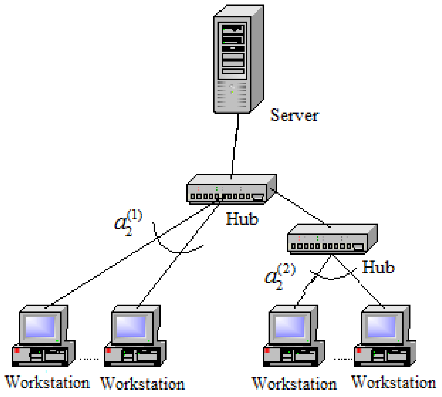
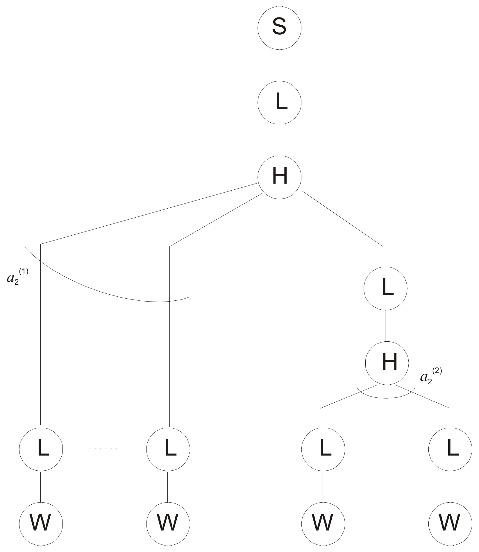
2. Representation of a Technical Equipment of a Local Area Computer Network in the Form of a Hierarchical Ramified System

The reliability issues are very important at the development stage and application of systems of different kinds in the industry. The calculation of reliability characteristics is rather difficult due to a great number of factors and general statistical nature of reliability.

As an example, we consider a technical equipment of a computer network [42,43,44,45] of the Ethernet 10 Base-T standard, which includes a server, two hubs, and workstations (Figure 1). We can update the network configuration with Ethernet 100 Base-T or Ethernet 1000 Base-T. However, in this case, we analyze the existing network.

A municipal firm has placed 20 workstations, namely seven workstations are connected to the server by the 8-port hub (the 1st hub), and the other 13 workstations are directly connected to the 16-port hub (the 2nd hub). Only the 8-port hub is directly connected to the server, and both hubs are connected with each other. Therefore, the 8-port hub can be considered to be basic. The place, where 13 workstations are placed, is remote from the server at a distance, which does not make it possible to connect them to the basic hub due to a limitation of the Ethernet 10 Base-T standard on the length of a communication line (no more than 100 m) between directly connected nodes for twisted pair cabling. This explains the use of the second hub. The place, where there are workstations connected to the basic hub, is limited in the area. No more than 7 workstations may be put over there. As we can see in standard IEEE 802.3 [46], if a twisted pair is used for the connection, the maximum length of the segment is 100 m (the same in all cases, for Ethernet 10 Base-T, Ethernet 100 Base-T, and Ethernet 1000 Base-T).

In Figure 1, $a_2^{\left(1\right)},a_2^{\left(2\right)}$ denote counts of workstations directly connected to the first (basic) hub and to the second hub, correspondingly. The following inequalities are fulfilled.

$$a_2^{\left(1\right)}\le 7,a_2^{\left(2\right)}\le 16,a_2^{\left(1\right)}<a_2^{\left(2\right)}.$$

(1)

The technical equipment of this local area computer network can be represented in the form of a hierarchical ramified system shown in Figure 2.

The server, hubs, workstations, and communication lines are the main blocks of the system in terms of reliability. If the server or the basic hub fails, all the systems can be considered inoperable. If the second hub fails, all the workstations, connected to it, can be considered inoperative.

3. Reliability Characteristics of Elements of the System

The investigator’s task is to fit a distribution of the probability of a failure-free operation that maintains a model’s adequacy for processes of the device’s lifetime. The server and workstations include electronic units, which can be considered ageless, as well as mechanical units, that yield exhaustion. In case of aging or exhaustion of elements, their lifetimes are described by the Weibull distribution [47,48,49,50]. The lifetimes of electronic units of the server and the lifetimes of workstations are described by the exponential distribution and the lifetimes of mechanical units can be described by the Weibull distribution.

In the process of constructing a mathematical model, we use the notation depicted in

Table 1. Nomenclature of the variables and parameters used in the model.

Name	Description	Units
$a_2^{\left(1\right)}$	The number of workstations directly connected to the first hub	-
$a_2^{\left(2\right)}$	The number of workstations directly connected to the second hub
$t$	A moment of time when calculation is conducted	hours
$p_s$	The probability of failure-free operation of a server
${\lambda }_0$	Failure intensity, a parameter of the exponential distribution for the probability of failure-free operation of electronic parts of a server	$\frac{1}{hours}$.
${\lambda }_1$	Failure intensity, a scale parameter of the Weibull distribution for the probability of failure-free operation of mechanical parts of a server	$\frac{1}{hours}$.
${\beta }_1$	An aging coefficient (parameter of the Weibull distribution for the probability of failure-free operation of mechanical parts of a server)	-
$p_L$	The probability of failure-free operation of a communication line as an ageless element	-
${\lambda }_2$	Failure intensity, a parameter of the exponential distribution for probability of failure-free operation of a communication line	$\frac{1}{hours}$.
$p_H$	The probability of failure-free operation of a hub
${\lambda }_3$	Failure intensity, a parameter of the exponential distribution for probability of failure-free operation of a hub	$\frac{1}{hours}$.
$p_W$	The probability of failure-free operation of a workstation
${\lambda }_4$	Failure intensity, a parameter of the exponential distribution for probability of failure-free operation of electronic parts of a workstation	$\frac{1}{hours}$.
${\lambda }_5$	Failure intensity, a scale parameter of the Weibull distribution for probability of failure-free operation of mechanical parts of a workstation	$\frac{1}{hours}$.
${\beta }_5$	An aging coefficient (parameter of the Weibull distribution for probability of failure-free operation of mechanical parts of a workstation)	-
$x_2$	The number of working output elements (2nd level)	-
$x_2^{\left(1\right)}$	The number of working output elements in the first branch (2nd level)	-
$x_2^{\left(2\right)}$	The number of working output elements in the second branch (2nd level)	-
$p_0$	The probability of failure-free operation of the elements at the 0-level (the first hub, server, and communication line)	-
$p_1$	The probability of failure-free operation of the elements at the first level (the second hub and communication line)	-
$p_2$	The probability of failure-free operation of the workstations, 2nd level	-
$S_2\left(z\right)$	The generating function
$P_2\left(x_2\right)$	A probability distribution of the count of the working output elements of the system	-
$P_2\left(x_2,t\right)$	The dependence of probability regarding the count of working output elements of the system upon time	-
$k$	The number of working output elements (availability condition - no less than $k$ output elements operate)	-
$K_{G2}\left(k,t\right)$	The availability function of the system
$T_2\left(x_2\right)$	The duration of the system’s stay in the state of $x_2$ operating output elements	hours
$T_{G2}\left(k\right)$	The duration of the system’s stay in the prescribed availability condition $k$	hours
$Q_2\left(k,t\right)$	The failure probability in the prescribed availability condition $k$	-
$a_2\left(k,t\right)$	Failure frequency in the prescribed availability condition $k$	$\frac{1}{hours}$
${\lambda }_2\left(k,t\right)$	Failure rate in the prescribed availability condition $k$	$\frac{1}{hours}$

.

Therefore, the probability of failure-free operation of a server is given by:

$$p_s\left(t\right)=e^{-{\lambda }_{0}t}{e}^{-{\lambda }_1{t}^{{\beta }_1}},$$

(2)

where ${\lambda }_0$ is a parameter of the exponential distribution for the probability of failure-free operation of electronic parts of a server, ${\lambda }_1$, ${\beta }_1$ are parameters of the Weibull distribution for the probability of failure-free operation of mechanical parts of a server, ${\lambda }_1$ is a scale parameter, and ${\beta }_1$ is an aging coefficient.

The probability of failure-free operation of a communication line as an ageless element is described by the exponential distribution.

$$p_L\left(t\right)=e^{-{\lambda }_{2}t},$$

(3)

where ${\lambda }_2$ is a parameter of the exponential distribution for the probability of failure-free operation of a communication line.

Hubs are electronic devices that can be considered ageless. The probability of failure-free operation of a hub is described by the exponential distribution.

$$p_H\left(t\right)=e^{-{\lambda }_{3}t},$$

(4)

where ${\lambda }_3$ is a parameter of the exponential distribution for the probability of failure-free operation of a hub.

The probability of failure-free operation of a workstation can be written in the form:

$$p_W\left(t\right)=e^{-{\lambda }_{4}t}{e}^{-{\lambda }_5{t}^{{\beta }_5}},$$

(5)

where ${\lambda }_4$ is a parameter of the exponential distribution for the probability of a failure-free operation of electronic parts of a workstation. ${\lambda }_5$, ${\beta }_5$ are parameters of the Weibull distribution for the probability of a failure-free operation of mechanical parts of a workstation, ${\lambda }_5$ is a scale parameter, and ${\beta }_5$ is an aging coefficient.

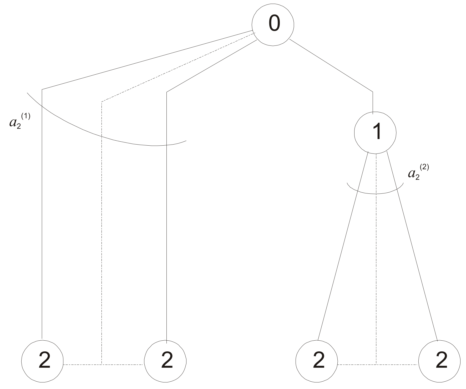
4. Contraction of Structure of the Hierarchical Ramified System

For simplification of calculations, it is necessary to reduce (contract) a hierarchical ramified system at the beginning. For this purpose, we merge elements, that do not ramify, into one element. The system will be simplified to a form shown in Figure 3, where elements are designated by integers that are numbers of levels where these elements are located.

In this system, the probabilities of failure-free operation of the elements are calculated as follows:

$$p_0=p_S{p}_L{p}_H, p_1=p_L{p}_H, p_2=p_L{p}_W,$$

(6)

where $p_0$ is for a hub of the 0-level (basic hub, the first hub), $p_1$ is for a hub of the 1-level (the second hub), $p_2$ are for workstations, level 2. Here, we use the same notations $p_S, p_L, p_H, p_W$ as in Equations (2)–(5).

The obtained hierarchical structure is based on the functional purpose of individual elements. Accordingly, the reliability properties of the elements of one level are the same. Therefore, in the presented example, the elements are distributed by levels exactly like that (all the workstations are at one level-number 2 in the Figure 3, and the hubs-at the other two levels, number 0 and 1). Considering the reliability properties of the elements of the hierarchical structure of the network this way, it is more convenient to develop a mathematical model, perform calculations, and automate the calculation process.

5. Construction of the Generation Function and Determination of Probabilistic Reliability Characteristics of the System on the Basis of This Function

According to the binomial theorem, the generating function is written in the form of the following sum of products.

$$\begin{array}{c}{S}_2\left(z\right)=p_0{\displaystyle \sum _{x_1^{\left(2\right)}=0}^1}{p}_1^{x_1^{\left(2\right)}}{(p_{2}z+q_2)}^{a_2^{\left(2\right)}{x}_1^{\left(2\right)}}{q}_1^{1-x_1^{\left(2\right)}} {\displaystyle \sum _{x_2^{\left(1\right)}=0}^{a_2^{\left(1\right)}}}{C}_{a_2^{\left(1\right)}}^{x_2^{\left(1\right)}}{p}_2^{x_2^{\left(1\right)}}{q}_2^{a_2^{\left(1\right)}-x_2^{\left(1\right)}}{z}^{x_2^{\left(1\right)}}+q_0\\ ={\displaystyle \sum _{x_1^{\left(2\right)}=0}^1}{\displaystyle \sum _{x_2^{\left(2\right)}=0}^{a_2^{\left(2\right)}{x}_1^{\left(2\right)}}}{\displaystyle \sum _{x_2^{\left(1\right)}=0}^{a_2^{\left(1\right)}}}{C}_{a_2^{\left(2\right)}{x}_1^{\left(2\right)}}^{x_2^{\left(2\right)}}{C}_{a_2^{\left(1\right)}}^{x_2^{\left(1\right)}}{p}_1^{x_1^{\left(2\right)}}{q}_1^{1-x_1^{\left(2\right)}}{p}_2^{x_2^{\left(1\right)}+x_2^{\left(2\right)}}{q}_2^{a_2^{\left(2\right)}{x}_1^{\left(2\right)}+a_2^{\left(1\right)}-x_2^{\left(1\right)}-x_2^{\left(2\right)}}{z}^{x_2^{\left(1\right)}+x_2^{\left(2\right)}}+q_0\end{array}$$

(7)

where $x_1^{\left(2\right)}$ is a count of working elements of level 1, $x_2^{\left(1\right)}$ is a count of the working elements of level 2 that belong to the first branch, and $x_2^{\left(2\right)}$ is a count of the working elements of level 2 that belong to the second branch.

On the basis of the generating function (7), we put down an expression for a probability distribution $P_2\left(x_2\right)$ of the count of the working output elements of the system. In addition, we take into account that the general count $x_2$ of working output elements of the system equals a sum of working elements in two branches. Hence, $x_2^{\left(2\right)}=x_2-x_2^{\left(1\right)}$.

We also take into the account that count $x_1^{\left(2\right)}$ of working elements of level 1 cannot be less than $\frac{x_2^{\left(2\right)}}{a_2^{\left(2\right)}}$, the count $x_2^{\left(1\right)}$ of working elements of level 2 that belong to the first branch cannot be more than both $a_2^{\left(1\right)}$ and $x_2$, and cannot be less than $x_2-a_2^{\left(2\right)}$ provided that $x_2>a_2^{\left(2\right)}$.

$$P_2\left(x_2\right)=p_0{\displaystyle \sum }_{x_2^{\left(1\right)}=\max \{0,x_2-a_2^{\left(2\right)}\}}^{\min \left\{x_{2,}{a}_2^{\left(1\right)}\right\}}{\displaystyle \sum }_{x_1^{\left(2\right)}=ceil\left(\frac{x_2-x_2^{\left(1\right)}}{a_2^{\left(2\right)}}\right)}^1{C}_{a_2^{\left(2\right)}{x}_1^{\left(2\right)}}^{x_2-x_2^{\left(1\right)}}{C}_{a_2^{\left(1\right)}}^{x_2^{\left(1\right)}}{p}_1^{x_1^{\left(2\right)}}{q}_1^{1-x_1^{\left(2\right)})}{p}_2^{x_2}{q}_2^{a_2^{\left(2\right)}{x}_1^{\left(2\right)}+a_2^{\left(1\right)}-.x_2}$$

(8)

Under the conditions $0<x_2\le a_2^{\left(1\right)}+a_2^{\left(2\right)}$, $a_2^{\left(1\right)}<a_2^{\left(2\right)}$, we obtain:

At $x_2=0$ the right side of Equation (8) should increase by $q_0$.

We pass to dependence of probability of the count of working output elements of the system upon time. Substituting Equations (3)–(5) into (6), we obtain:

$$p_0=e^{-\left({\lambda }_0+{\lambda }_2+{\lambda }_3\right)t-{\lambda }_1{t}^{{\beta }_1}}, p_1=e^{-\left({\lambda }_2+{\lambda }_3\right)t}, p_2=e^{-\left({\lambda }_2+{\lambda }_4\right)t-{\lambda }_5{t}^{{\beta }_5}}.$$

(9)

Substituting Equation (9) into Equation (8), we obtain under the conditions $0<x_2\le a_2^{\left(1\right)}+a_2^{\left(2\right)}$, $a_2^{\left(1\right)}<a_2^{\left(2\right)}$:

$$\begin{array}{l}{P}_2\left(x_2,t\right)=e^{-\left({\mathsf{\lambda }}_0+{\mathsf{\lambda }}_2+{\mathsf{\lambda }}_3\right)t-{\mathsf{\lambda }}_1{t}^{{\mathsf{\beta }}_1}}{{\displaystyle \sum }}_{x_2^{\left(1\right)}=\max \{0,x_2-a_2^{\left(2\right)}\}}^{\min \left\{x_{2,}{a}_2^{\left(1\right)}\right\}}{{\displaystyle \sum }}_{x_1^{\left(2\right)}=ceil\left(\frac{x_2-x_2^{\left(1\right)}}{a_2^{\left(2\right)}}\right)}^1{C}_{a_2^{\left(2\right)}{x}_1^{\left(2\right)}}^{x_2-x_2^{\left(1\right)}}\times C_{a_2^{\left(1\right)}}^{x_2^{\left(1\right)}}{e}^{-\left({\lambda }_2+{\lambda }_3\right)x_1^{\left(2\right)}t}\\ {\left(1-e^{-\left({\lambda }_2+{\lambda }_3\right)t}\right)}^{1-x_1^{\left(2\right)}}\times e^{-x_2\left(\left({\lambda }_2+{\lambda }_4\right)t+{\lambda }_5{t}^{{\beta }_5}\right)}{\left(1-e^{-\left({\lambda }_2+{\lambda }_4\right)t-{\lambda }_5{t}^{{\beta }_5}}\right)}^{a_2^{\left(2\right)}{x}_1^{\left(2\right)}+a_2^{\left(1\right)}-x_2}\end{array}$$

(10)

At $x_2=0$, the right side of Equation (10) should increase by $1-e^{-\left({\lambda }_0+{\lambda }_2+{\lambda }_3\right)t-{\lambda }_1{t}^{{\beta }_1}}$. The probability that there are no less than $k$ working output elements when $0<k\le \left(a_2^{\left(1\right)}+a_2^{\left(2\right)}\right)$ is the availability function of the system. Under the condition $a_2^{\left(1\right)}<a_2^{\left(2\right)}$, this function is written in the following way.

$$\begin{array}{c}{K}_{G2}\left(k,t\right)={{\displaystyle \sum }}_{x_2=k}^{a_2^{\left(1\right)}+a_2^{\left(2\right)}}{P}_2\left(x_2,t\right)={{\displaystyle \sum }}_{x_2=k}^{a_2^{\left(1\right)}+a_2^{\left(2\right)}}{e}^{-\left({\lambda }_0+{\lambda }_2+{\lambda }_3\right)t-{\lambda }_1{t}^{{\beta }_1}}\times \\ {{\displaystyle \sum }}_{x_2^{\left(1\right)}=\max \{0,x_2-a_2^{\left(2\right)}\}}^{\min \left\{x_{2,}{a}_2^{\left(1\right)}\right\}}{{\displaystyle \sum }}_{x_1^{\left(2\right)}=ceil\left(\frac{x_2-x_2^{\left(1\right)}}{a_2^{\left(2\right)}}\right)}^1{C}_{a_2^{\left(2\right)}{x}_1^{\left(2\right)}}^{x_2-x_2^{\left(1\right)}}{C}_{a_2^{\left(1\right)}}^{x_2^{\left(1\right)}}{e}^{-\left({\lambda }_2+{\lambda }_3\right)x_1^{\left(2\right)}t}\times \\ {\left(1-e^{-\left({\lambda }_2+{\lambda }_3\right)t}\right)}^{1-x_1^{\left(2\right)}}{e}^{-x_2\left(\left({\lambda }_2+{\lambda }_4\right)t+{\lambda }_5{t}^{{\beta }_5}\right)}{\left(1-e^{-\left({\lambda }_2+{\lambda }_4\right)t-{\lambda }_5{t}^{{\beta }_5}}\right)}^{a_2^{\left(2\right)}{x}_1^{\left(2\right)}+a_2^{\left(1\right)}-x_2}.\end{array}$$

(11)

It should be noted that, if new structural elements/levels are added to the system (e.g., WiFi routers, BT devices, LTE, etc.), then the structure of the mathematical model will be analogous, but it will contain more parameters and variables. Calculations will be more complicated and time-consuming.

6. Calculations of Time Reliability Characteristics of the System

We pass to two main time reliability characteristics of the system: the average duration of the system’s stay in each of its states and the average duration of the system’s stay in the prescribed availability condition.

The duration of the system’s stay in the state of $x_2$ operating output elements is obtained by integrating the expression for the probability distribution of the count of output working elements with respect to $t$ from 0 to $\infty$.

Under the conditions $0<\le a_2^{\left(1\right)}+a_2^{\left(2\right)}$, $a_2^{\left(1\right)}<a_2^{\left(2\right)},$ we obtain:

$$T_2\left(x_2\right)={{\displaystyle \int }}_0^{\infty }{P}_2\left(x_2,t\right)dt,$$

(12)

where $P_2\left(x_2,t\right)$ is calculated by Equation (10).

The duration of the system’s stay in the prescribed availability condition $k$, which means that no less than $k$ output elements operate, equals a sum of durations of the system’s stay in states over the count of output elements from $k$ to $a_2^{\left(1\right)}+a_2^{\left(2\right)}$. Under the conditions $0<k\le a_2^{\left(1\right)}+a_2^{\left(2\right)}$, we obtain:

$$T_{G2}\left(k\right)={{\displaystyle \sum }}_{x_2=k}^{a_2^{\left(1\right)}+a_2^{\left(2\right)}}{T}_2\left(x_2\right),$$

(13)

where $T_2\left(x_2\right)$ is calculated by Equation (12).

7. Calculations of Conventional Reliability Characteristics for Unrestorable Ramified Systems

Under the prescribed availability condition, on the basis of the expression for the availability function of the system, it is possible to estimate the system’s reliability by means of three conventional characteristics specified by standards for unrestorable systems: the failure probability, the failure frequency, and the failure rate.

The failure probability in the prescribed availability condition k, where $0<k\le a_2^{\left(1\right)}+a_2^{\left(2\right)},a_2^{\left(1\right)}<a_2^{\left(2\right)}$, is written in the following way:

$$\begin{array}{c}{Q}_2\left(k,t\right)=1-K_{G2}\left(k,t\right)=1-{{\displaystyle \sum }}_{x_2=k}^{a_2^{\left(1\right)}+a_2^{\left(2\right)}}{e}^{-\left({\lambda }_0+{\lambda }_2+{\lambda }_3\right)t-{\lambda }_1{t}^{{\beta }_1}}\times \\ {{\displaystyle \sum }}_{x_2^{\left(1\right)}=\max \{0,x_2-a_2^{\left(2\right)}\}}^{\min \left\{x_{2,}{a}_2^{\left(1\right)}\right\}}{{\displaystyle \sum }}_{x_1^{\left(2\right)}=ceil\left(\frac{x_2-x_2^{\left(1\right)}}{a_2^{\left(2\right)}}\right)}^1{C}_{a_2^{\left(2\right)}{x}_1^{\left(2\right)}}^{x_2-x_2^{\left(1\right)}}{C}_{a_2^{\left(1\right)}}^{x_2^{\left(1\right)}}{e}^{-\left({\lambda }_2+{\lambda }_3\right)x_1^{\left(2\right)}t}\times \\ {\left(1-e^{-\left({\lambda }_2+{\lambda }_3\right)t}\right)}^{1-x_1^{\left(2\right)}}{e}^{-x_2\left(\left({\lambda }_2+{\lambda }_4\right)t+{\lambda }_5{t}^{{\beta }_5}\right)}{\left(1-e^{-\left({\lambda }_2+{\lambda }_4\right)t-{\lambda }_5{t}^{{\beta }_5}}\right)}^{a_2^{\left(2\right)}{x}_1^{\left(2\right)}+a_2^{\left(1\right)}-x_2}.\end{array}$$

(14)

For calculation of the failure frequency in the prescribed availability condition $k$, where $0<k\le a_2^{\left(1\right)}+a_2^{\left(2\right)}$, $a_2^{\left(1\right)}<a_2^{\left(2\right)}$, we obtain:

$$a_2\left(k,t\right)=-\frac{d{K}_{G2}\left(k,t\right)}{dt},$$

(15)

where $K_{G2}\left(k,t\right)$ is calculated by Equation (11).

The main characteristic for reliability evaluation of unrestorable systems, according to standards, is the failure rate [51,52]. Under the prescribed availability condition $k$ and under the conditions $0<k\le a_2^{\left(1\right)}+a_2^{\left(2\right)}$, $a_2^{\left(1\right)}<a_2^{\left(2\right)},$ we obtain:

$${\lambda }_2\left(k,t\right)=\frac{a_2\left(k,t\right)}{K_{G2}\left(k,t\right)},$$

(16)

where $a_2\left(k,t\right)$ and $K_{G2}\left(k,t\right)$ are calculated by Equations (15) and (11), respectively.

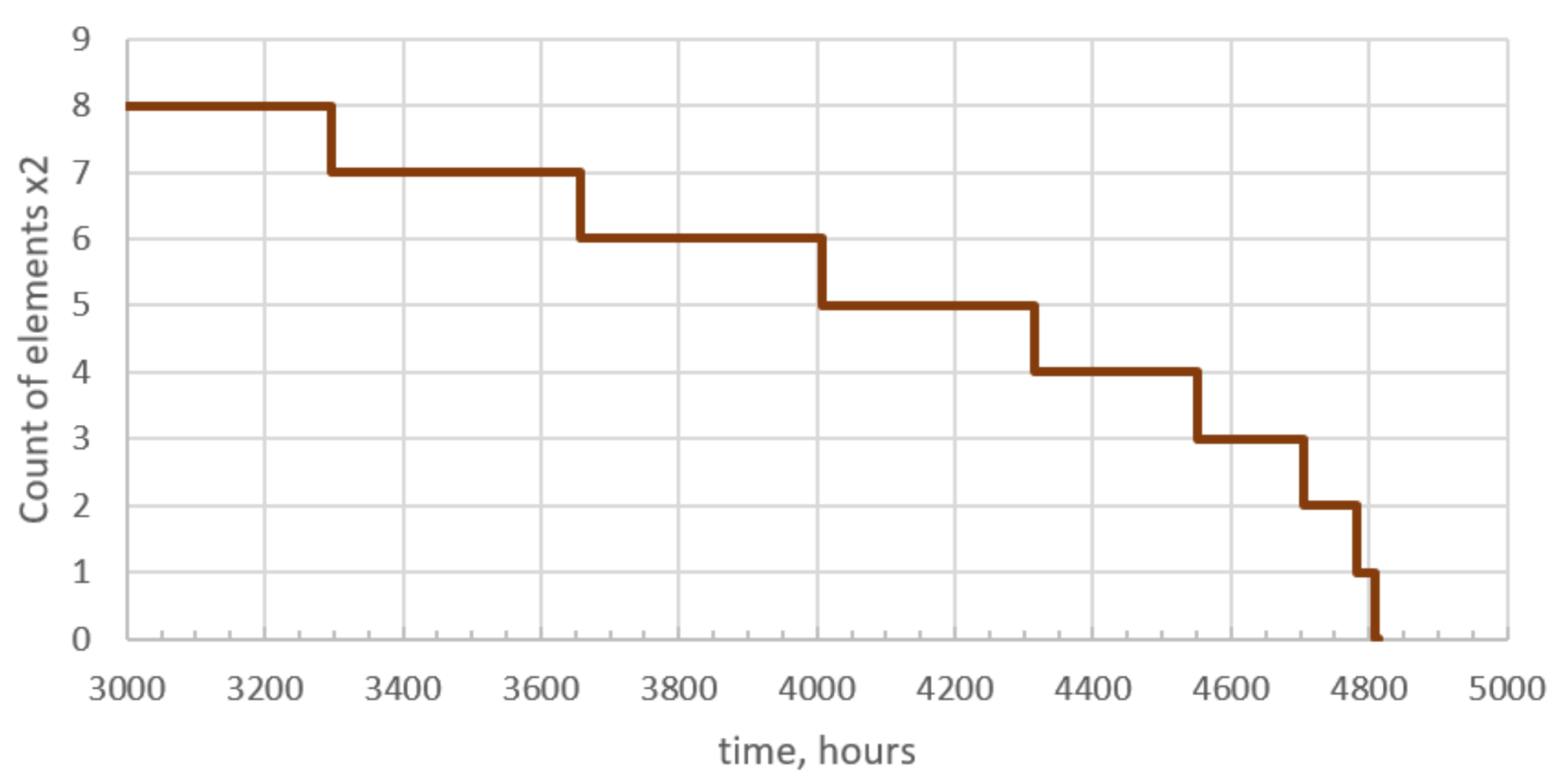
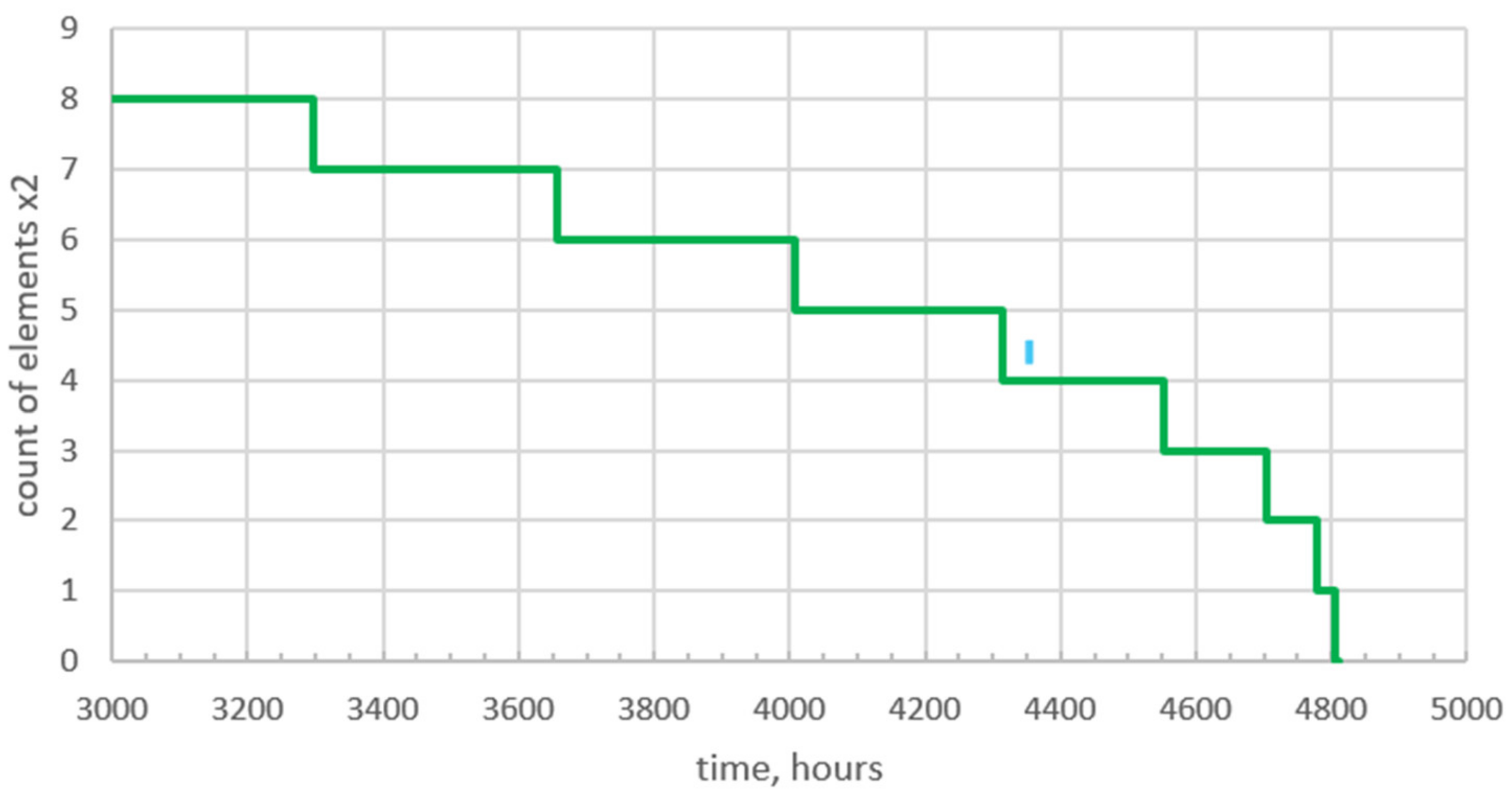
8. An Example of Calculations

The input data for calculating the reliability characteristics of the system shown in Figure 1 are the parameters of the server, the hubs, the workstations, and communication line, namely: ${\lambda }_0$, ${\lambda }_1$, ${\beta }_1$, ${\lambda }_2$, ${\lambda }_3$, ${\lambda }_4$, ${\lambda }_5$, ${\beta }_5$, $a_2^{\left(1\right)},a_2^{\left(2\right)}$, $x_2$ (they are described in detail in Table 1) and $t$ is a moment of time when calculation is conducted.

For the server, when the average operating time to failure is 172,199 h [53], we obtain:

$${\lambda }_0=5,807\ast {10}^{-6}\frac{1}{hours}.$$

(17)

For mechanical parts of the server (e.g., cooler with the average operating time to failure at about 100,000 h [54]), an aging coefficient should be chosen between 1.1 and 1.3. At ${\beta }_1=1,2$ for the given average operating time to failure, we obtain:

$${\lambda }_1=9,2927\ast {10}^{-7}\frac{1}{hours}.$$

(18)

Analogously for the workstations, proceeding from the average operating time to failure at 8766 h, we obtain:

$${\lambda }_4=1.14\ast {10}^{-4}\frac{1}{hours}, {\lambda }_5=2,80651\ast {10}^{-5}\frac{1}{hours}, {\beta }_5=1,2.$$

(19)

For the communication lines, granting stationary service conditions, it is necessary to assign:

$${\lambda }_2=6,12105\ast {10}^{-8}\frac{1}{hours}.$$

(20)

Proceeding from the average operating time to failure of the hub at 492,096 h (we consider 16-Port Fast Ethernet unmanaged switch DES-1016D [55]) and taking into account that the 8-port hub has almost the same operating time to failure (for example, D-Link DGS 1008D 8-port switch [56]), we obtain:

$${\lambda }_3=2,03\ast {10}^{-6}\frac{1}{hours}.$$

(21)

As a result of calculations, it is possible to obtain the following main output data [48,49]: the probability distribution of a count of operating output elements, the availability function, the duration of the system’s stay in each of its working states, the duration of the system’s stay in the prescribed availability condition, the failure frequency in the prescribed availability condition, and the failure rate in the prescribed availability condition.

The results of calculations of the availability function, the failure frequency, and the failure rate of the system in the prescribed availability condition and under the condition $0\le t\le 5000$ h are shown in Figure 4, Figure 5 and Figure 6.

For validation of the results, we take into consideration conditions (1) and the conditions below.

$$a_2^{\left(1\right)}+a_2^{\left(2\right)}=20.$$

(22)

The choice of the ramification coefficients $a_2^{\left(1\right)}$, $a_2^{\left(2\right)},$ which ensure the highest reliability of the system under the conditions (1) and (22).

The decision about an optimal variant of placement of 20 workstations under the conditions (1) and (22) should be made on the basis of the following reliability characteristics of the system: the availability function, the failure frequency in the prescribed availability condition, the failure rate in the prescribed availability condition, and the duration of the system’s stay in the prescribed availability condition. As a result of the calculations, it appears that, under the condition $0\le t\le 5000$ h, the availability function, the failure frequency, and the failure rate in the prescribed availability condition do not depend on the variant of placement that responds to the conditions (1) and (22).

The average duration of the system’s stay in the state of $x_2$ working output elements of the system under the condition $8\le x_2\le 20$ does not depend on the variant of placement responding to the conditions (1) and (22).

All the 20 output elements of the system will operate on the average for 242.28 h from the beginning of the system’s operation. Afterward, one of the elements will fail and 19 output elements will operate on an average of 475.27 h. After failure of the second output element, 18 output elements will operate, on average, for 708.79 h.

In Figure 7, Figure 8, Figure 9 and Figure 10, the fragments of histograms of the system’s operation in the course of time under different variants of placement that satisfy the conditions (1) and (22) are presented. From the initial moment of time (t = 0) and up to t = 3000 h—the value is constant, that is why it is not shown in Figure 7, Figure 8, Figure 9 and Figure 10 (for better visualization). These figures demonstrate that, under the condition $1\le x_2\le 7,$ a maximum value of a moment of time, until which no less than $x_2$ output elements operate, is reached when $a_2^{\left(1\right)}=4$, $a_2^{\left(2\right)}=16$. Thus, the optimal variant of placement of output elements of the system is connecting four workstations to the basic hub and 16 workstations to the second hub.

The analysis of the obtained results shows that, on average, they will remain in the system:

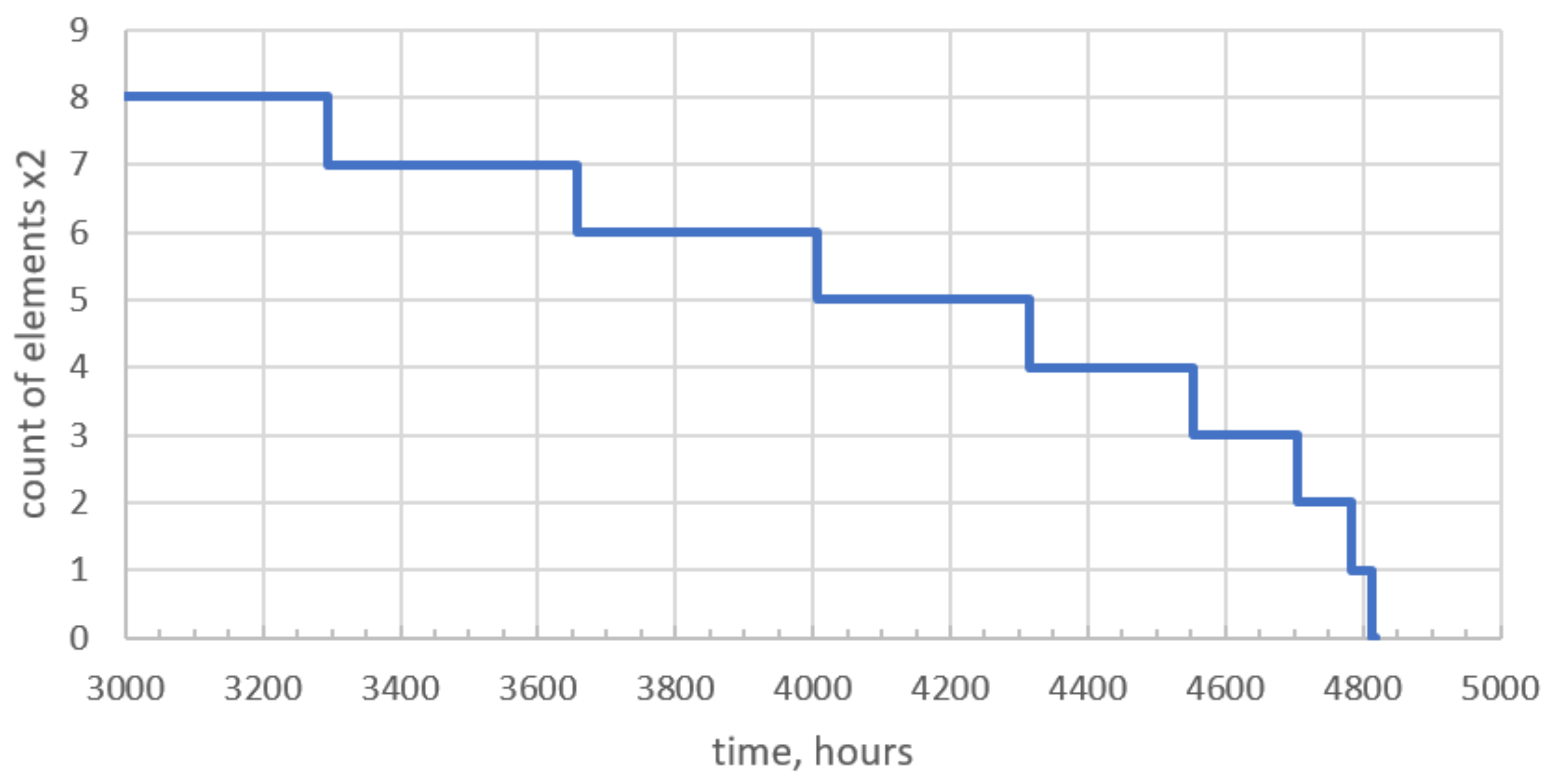
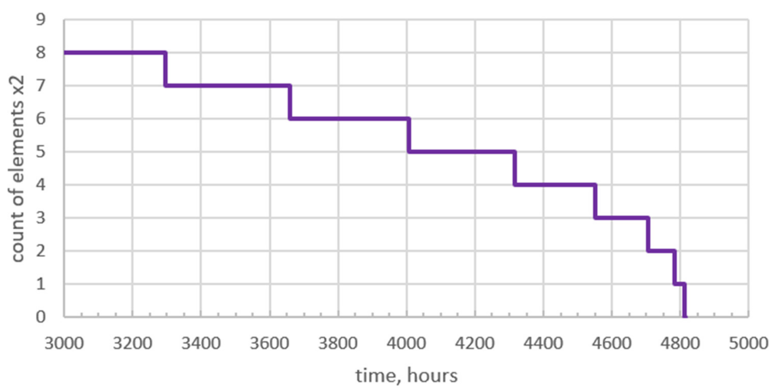
• $x_2$ = 6 operating output elements at t = 3658 h (if $a_2^{\left(1\right)}=4$, $a_2^{\left(2\right)}=16$), t = 3658 h ($a_2^{\left(1\right)}=5$, $a_2^{\left(2\right)}=15$), t = 3658 h ($a_2^{\left(1\right)}=6$, $a_2^{\left(2\right)}=14$), t = 3658 h ($a_2^{\left(1\right)}=7$, $a_2^{\left(2\right)}=13$);
• $x_2$ = 5 operating output elements at t = 4315 h ($a_2^{\left(1\right)}=4$, $a_2^{\left(2\right)}=16$), t = 4315 h ($a_2^{\left(1\right)}=5$, $a_2^{\left(2\right)}=15$), t = 4315 h ($a_2^{\left(1\right)}=6$, $a_2^{\left(2\right)}=14$), t = 4315 h ($a_2^{\left(1\right)}=7$, $a_2^{\left(2\right)}=13$);
• $x_{2 }$ = 4 operating output elements at t = 4552 h ($a_2^{\left(1\right)}=4$, $a_2^{\left(2\right)}=16$), t = 4552 h ($a_2^{\left(1\right)}=5$, $a_2^{\left(2\right)}=15$), t = 4552 h ($a_2^{\left(1\right)}=6$, $a_2^{\left(2\right)}=14$), t = 4552 h ($a_2^{\left(1\right)}=7$, $a_2^{\left(2\right)}=13$);
• $x_2$ = 3 operating output elements at t = 4705 h ($a_2^{\left(1\right)}=4$, $a_2^{\left(2\right)}=16$), t = 4705 h ($a_2^{\left(1\right)}=5$, $a_2^{\left(2\right)}=15$), t = 4705 h ($a_2^{\left(1\right)}=6$, $a_2^{\left(2\right)}=14$), t = 4704 h ($a_2^{\left(1\right)}=7$, $a_2^{\left(2\right)}=13$);
• $x_2$ = 2 operating output elements at t = 4783 h ($a_2^{\left(1\right)}=4$, $a_2^{\left(2\right)}=16$), t = 4783 h ($a_2^{\left(1\right)}=5$, $a_2^{\left(2\right)}=15$), t = 4782 h ($a_2^{\left(1\right)}=6$, $a_2^{\left(2\right)}=14$), t = 4780 h ($a_2^{\left(1\right)}=7$, $a_2^{\left(2\right)}=13$);
• $x_2$ = 1 operating output element at t = 4812 h ($a_2^{\left(1\right)}=4$, $a_2^{\left(2\right)}=16$), t = 4811 h ($a_2^{\left(1\right)}=5$, $a_2^{\left(2\right)}=15$), t = 4809 h ($a_2^{\left(1\right)}=6$, $a_2^{\left(2\right)}=14$), t = 4806 h ($a_2^{\left(1\right)}=7$, $a_2^{\left(2\right)}=13$);
• $x_2$ = 0 operating output elements at t = 4818 h ($a_2^{\left(1\right)}=4$, $a_2^{\left(2\right)}=16$), t = 4816 h ($a_2^{\left(1\right)}=5$, $a_2^{\left(2\right)}=15$), t = 4814 h ($a_2^{\left(1\right)}=6$, $a_2^{\left(2\right)}=14$), t = 4811 h ($a_2^{\left(1\right)}=7$, $a_2^{\left(2\right)}=13$).

Thus, no later than in 4818 h, on average, the system will fail at $a_2^{\left(1\right)}=4$, $a_2^{\left(2\right)}=16$.

9. Conclusions

A technical equipment of a local area computer network, whose main blocks are a server, hubs, workstations, and communication lines, is considered as a hierarchical ramified system with aging elements. In order to simplify the calculations of reliability characteristics, this system is represented in contracted form as a hierarchical system with the bypath through one level, ramified to level 2.

Models in the form of expressions are constructed for calculations of the following:

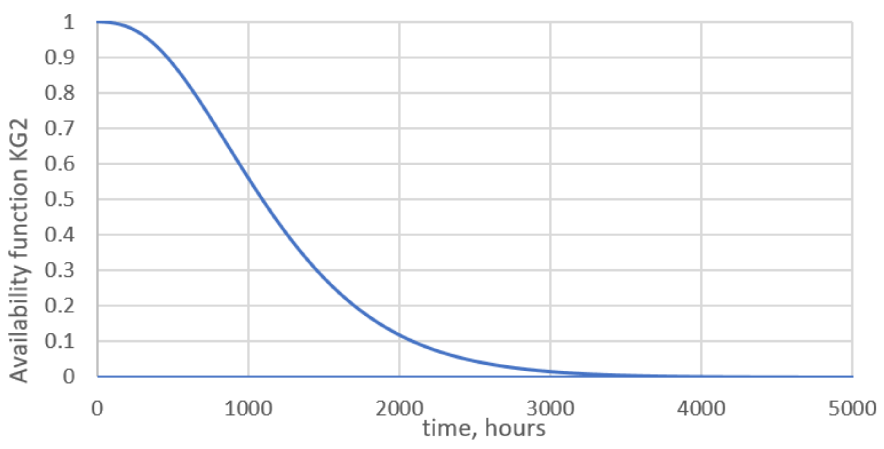
• probabilistic reliability characteristics of the system (the probability distribution of a count of operating output elements, the availability function);
• time reliability characteristics of the system (the duration of the system’s stay in each of its working states, the duration of the system’s stay in the prescribed availability condition);
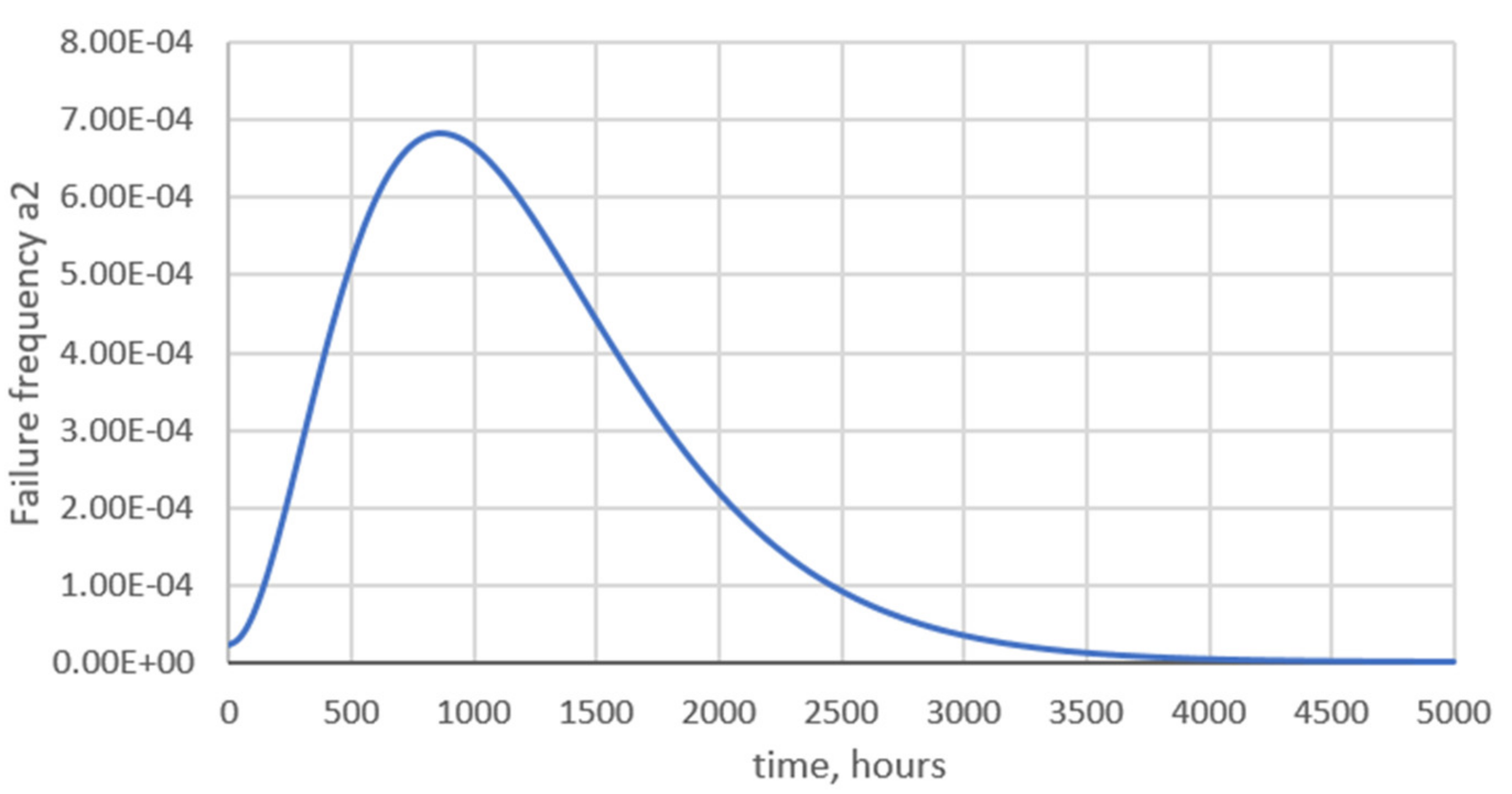
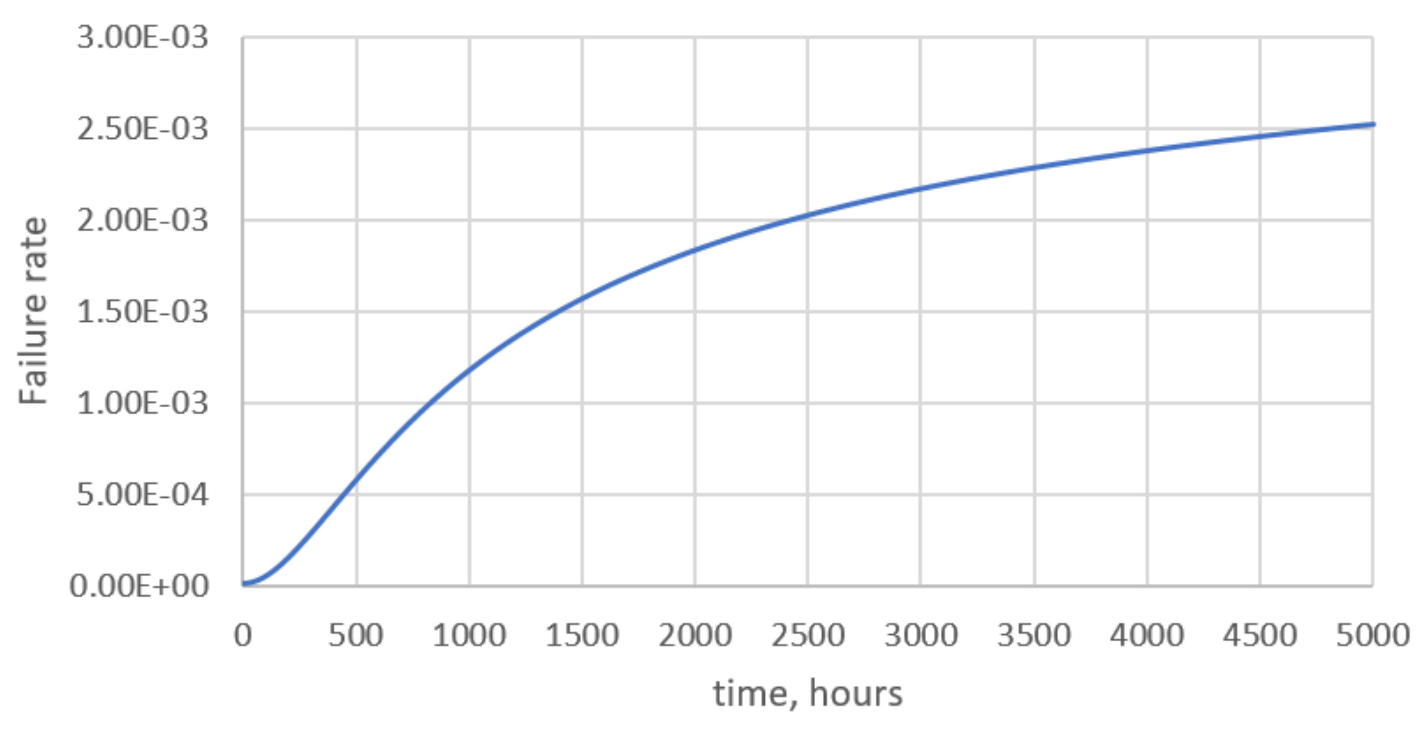
• conventional reliability characteristics specified by standards for unrestorable systems (the failure probability in the prescribed availability condition, the failure frequency in the prescribed availability condition, and the failure rate in the prescribed availability condition).

The results of calculations of reliability characteristics are presented for the case of a technical equipment of a local area computer network.

Without the use of reliability characteristics, it is impossible to settle a number of problems of systems’ design and operation, such as a selection of structure and rational redundancy, an organization of inspection monitoring, and preventive maintenance. It is necessary to work out the methods of reliability prognostication with regard to systems’ specific features, such as the possibility of structure rearrangement, and preservation of serviceability in case of partial failures at the expense of structural redundancy.

The analytical models, determining reliability parameters with high accuracy, have been developed for modern hierarchical systems widely used in technology. These models are based on the use of the Weibull distribution. The accuracy of the developed analytical models is determined by the errors of the input data. In addition, the proposed models, due to the regularity of such hierarchical systems, can help automate the process of their synthesis and can be used to explore the parameters of large systems. The study presented in the article can be generalized for hierarchical systems with more levels and elements at each level.

Thus, the model for determining the reliability parameters of hierarchical, multilevel, branched systems has been developed and is presented in this paper. The proposed model uses a system of analytical expressions, which allows us to determine the reliability parameters of the studied object with high accuracy and can be used for large, multi-level, hierarchical, ramified systems.

10. Prospects for Future Research

The future research of this theme will be focused on the following. First, we will work on the development of the generalized algorithm for automatic forming of the optimal/quasi-optimal placement based on the input data. Second, we plan to introduce several parameters into the model, which allow us to take into account different types of cabling (not only twisted pair, but an optical fiber and coaxial cable) as well as different reliability indicators of hubs and workstation connections.

References

1. Stapelberg, R.F. Handbook of Reliability, Availability, Maintainability and Safety in Engineering Design; Springer: London, UK, 2009. [Google Scholar]
2. Zhurakhivskyi, A.V.; Kinash, B.M.; Pastukh, O.R. Nadiinist Elektrychnykh System i Merezh: Navch. Posib; Vydavnytstvo Lvivckoi Politekhniky: Lviv, Ukraine, 2012. (in Ukrainian) [Google Scholar]
3. Song, K.Y.; Chang, I.H.; Pham, H. A Software Reliability Model with a Weibull Fault Detection Rate Function Subject to Operating Environments. Appl. Sci. 2017, 7, 983. [Google Scholar] [CrossRef] [Green Version]
4. Bobalo, Y.; Seniv, M.; Yakovyna, V.; Symets, I. Method of Reliability Block Diagram Visualization and Automated Construction of Technical System Operability Condition. Adv. Intell. Syst. Comput. III 2019, 871, 599–610. [Google Scholar]
5. Arnott, R.; Greenwald, B.; Stiglitz, J.E. Information and economic efficiency. Inf. Econ. Policy 1994, 6, 77–82. [Google Scholar] [CrossRef] [Green Version]
6. Kryvinska, N.; Bickel, L. Scenario-Based Analysis of IT Enterprises Servitization as a Part of Digital Transformation of Modern Economy. Appl. Sci. 2020, 10, 1076. [Google Scholar] [CrossRef] [Green Version]
7. Cheng, Q.; Zhao, H.; Zhao, Y. Machining accuracy reliability analysis of multi-axis machine tool based on Monte Carlo simulation. J. Intell. Manuf. 2015, 29, 191–209. [Google Scholar] [CrossRef]
8. Cheng, Q.; Wang, S.; Yan, C. Sequential Monte Carlo Simulation for Robust Optimal Design of Cooling Water System with Quantified Uncertainty and Reliability. Energy 2017, 118, 489–501. [Google Scholar] [CrossRef]
9. Han, Y.; Wen, Y.; Guo, C.; Huang, H. Incorporating Cyber Layer Failures in Composite Power System Reliability Evaluations. Energies 2015, 8, 9064–9086. [Google Scholar] [CrossRef] [Green Version]
10. Chen, B.J.; Chen, X.F.; Li, B. Reliability Estimation for Cutting Tool Based on Logistic Regression Model. J. Mech. Eng. 2011, 47, 158–164. [Google Scholar] [CrossRef]
11. Mitchell, R.; Chen, I. Modeling and Analysis of Attacks and Counter Defense Mechanisms for Cyber Physical Systems. IEEE Trans. Reliab. 2016, 65, 350–358. [Google Scholar] [CrossRef]
12. Sankaran, M.; Ruoxue, Z.; Natasha, S. Bayesian networks for system reliability reassessment. Struct. Saf. 2013, 23, 231–251. [Google Scholar]
13. Li, Y.F.; Huang, H.Z.; Mi, J.; Peng, W.; Han, X. Reliability analysis of multi-state systems with common cause failures based on Bayesian network and fuzzy probability. Ann. Oper. Res. 2019, 1–15. [Google Scholar] [CrossRef]
14. Chinnam, R.B.; Mohan, P. Online Reliability Estimation of Physical Systems Using Neural Networks and Wavelets. Int. J. Smart Eng. Syst. Des. 2002, 4, 253–264. [Google Scholar] [CrossRef]
15. Walls, L.; Alkali, B. Advances in Mathematical Modeling for Reliability; IOS Press: Amsterdam, The Netherland, 2008. [Google Scholar]
16. Huang, L. Lifetime Reliability for Load-Sharing Redundant Systems with Arbitrary failure Distributions. Reliab. IEEE Trans. On. 2010, 59, 319–330. [Google Scholar] [CrossRef] [Green Version]
17. Hardy, G.; Lucet, C.; Limnios, N. K-Terminal Network Reliability Measures with Binary Decision Diagrams. IEEE Trans. Reliab. 2007, 56, 506–515. [Google Scholar] [CrossRef]
18. Lefebvre, M. Basic Probability Theory with Applications; Springer: New York, NY, USA, 2009; p. 103. [Google Scholar]
19. Thomas, L.C. A survey of maintenance and replacement models for maintainability and reliability of multi-item systems. Reliab. Eng. 1986, 16, 297–309. [Google Scholar] [CrossRef]
20. Stefanovych, T.; Shcherbovskykh, S.; Droździel, P. The reliability model for failure cause analysis of pressure vessel protective fittings with taking into account load-sharing effect between valves. Diagnostyka 2015, 16, 17–24. [Google Scholar]
21. Catelani, M.; Ciani, L.; Venzi, M. Component Reliability Importance assessment on complex systems using Credible Improvement Potential. Microelectron. Reliab. 2016, 64, 113–119. [Google Scholar] [CrossRef]
22. Bagad, V.S.; Dhotre, I.A. Computer Networks; Technical Publications: Pune, India, 2009; 512p. [Google Scholar]
23. Behnke, S.; Rojas, R. Neural Abstraction Pyramid: A hierarchical image understanding architecture. In Proceedings of the International Joint Conference on Neural Networks, Anchorage, AK, USA, 4–9 May 1998; Volume 2, pp. 820–825. [Google Scholar]
24. Behnke, S. Related Work. In Hierarchical Neural Networks for Image Interpretation; Lecture Notes in Computer Science; Springer: Berlin/Heidelberg, Germany, 2003; Volume 2766, pp. 35–63. [Google Scholar]
25. Risteska Stojkoska, B.L.; Trivodaliev, K.V. A review of Internet of Things for smart home: Challenges and solutions. J. Clean. Prod. 2017, 140, 1454–1464. [Google Scholar] [CrossRef]
26. Hammi, B.; Khatoun, R.; Zeadally, S.; Fayad, A.; Khoukhi, L. Internet of Things (IoT) Technologies for Smart Cities. IET Res. J. 2017, 7, 1–13. [Google Scholar]
27. Boreiko, O.Y.; Teslyuk, V.M.; Zelinskyy, A.; Berezsky, O. Development of models and means of the server part of the system for passenger traffic registration of public transport in the “smart” city. East. Eur. J. Enterp. Technol. 2017, 1, 40–47. [Google Scholar] [CrossRef] [Green Version]
28. Teich, T.; Roessler, F.; Kretz, D.; Frank, S. Design of a Prototype Neural Network for Smart Homes and Energy Efficiency. Procedia Eng. 2014, 69, 603–609. [Google Scholar] [CrossRef] [Green Version]
29. Lytvyn, V.; Vysotska, V.; Mykhailyshyn, V.; Peleshchak, I.; Peleshchak, R.; Kohut, I. Intelligent system of a smart house. In Proceedings of the 3rd International Conference on Advanced Information and Communications Technologies, AICT, Lviv, Ukraine, 2–6 July 2019; pp. 282–287. [Google Scholar]
30. Bera, B.; Saha, S.; Das, A.K.; Vasilakos, A.V. Designing Blockchain-Based Access Control Protocol in IoT-Enabled Smart-Grid System. IEEE Internet Things J. 2021, 8, 5744–5761. [Google Scholar] [CrossRef]
31. Xu, X.; Sun, G.; Luo, L.; Cao, H.; Yu, H.; Vasilakos, A.V. Latency performance modeling and analysis for hyperledger fabric blockchain network. Inf. Process. Manag. 2021, 58, 102436. [Google Scholar] [CrossRef]
32. Andreotti, A.; Caiazzo, B.; Petrillo, A.; Santini, S.; Vaccaro, A. Hierarchical Two-Layer Distributed Control Architecture for Voltage Regulation in Multiple Microgrids in the Presence of Time-Varying Delays. Energies 2020, 13, 6507. [Google Scholar] [CrossRef]
33. Sydor, A.R.; Teslyuk, V.M.; Denysyuk, P.Y. Recurrent expressions for reliability indicators of compound electropower systems. Tech. Electrodyn. 2014, 4, 47–49. [Google Scholar]
34. Kwon, S. CLSTM: Deep Feature-Based Speech Emotion Recognition Using the Hierarchical ConvLSTM Network. Mathematics 2020, 8, 2133. [Google Scholar]
35. Ling, M.H.; Hu, X.W. Optimal design of simple step-stress accelerated life tests for one-shot devices under Weibull distributions. Reliab. Eng. Syst. Safety 2020, 193, 106630. [Google Scholar] [CrossRef]
36. Neumann, S.; Woll, L.; Feldermann, A. Modular System Modeling for Quantitative Reliability Evaluation of Technical Systems. Model. Identif. Control 2016, 37, 19–29. [Google Scholar] [CrossRef] [Green Version]
37. Bahrebar, S.; Zhou, D.; Rastayesh, S.; Wang, H.; Blaabjerg, F. Reliability assessment of power conditioner considering maintenance in a PEM fuel cell system. Microelectron. Reliab. 2018, 88, 1177–1182. [Google Scholar] [CrossRef]
38. Bender, E.; Bernstein, J.B.; Bensoussan, A. Reliability prediction of FinFET FPGAs by MTOL. Microelectron. Reliab. 2020, 114, 113809. [Google Scholar] [CrossRef]
39. Feng, X.; Raghavan, N.; Mei, S.; Dong, S.; Pey, K.L.; Wong, H. Statistical nature of hard breakdown recovery in high-κ dielectric stacks studied using ramped voltage stress. Microelectron. Reliab. 2018, 88, 164–168. [Google Scholar] [CrossRef]
40. Abd EL-Baset, A.A.; Ghazal, M.G.M. Exponentiated additive Weibull distribution. Reliab. Eng. Syst. Safety 2020, 193, 106663. [Google Scholar]
41. Zhu, T. Reliability estimation for two-parameter Weibull distribution under block censoring. Reliab. Eng. Syst. Safety 2020, 203, 107071. [Google Scholar] [CrossRef]
42. Dronyuk, I.; Fedevych, O.; Lizanets, D.; Kryvinska, N. An Overview of Ateb-Theory Mathematical Apparatus for Data Confidentiality in Medical Computer Networks. IDDM 2019, 2488, 175–184. [Google Scholar]
43. Auzinger, W.; Obelovska, K.; Stolyarchuk, R. A Revised Gomory-Hu Algorithm Taking Account of Physical Unavailability of Network Channels. In Computer Networks; Communications in Computer and Information Science; Gaj, P., Gumiński, W., Kwiecień, A., Eds.; Springer: Cham, Switzerland, 2020; Volume 1231, pp. 3–13. [Google Scholar]
44. Poniszewska-Maranda, A.; Kaczmarek, D.; Kryvinska, N. Studying usability of AI in the IoT systems/paradigm through embedding NN techniques into mobile smart service system. Computing 2018, 10, 1–25. [Google Scholar] [CrossRef]
45. Hamdan, M.; Hassan, E.; Abdelaziz, A.; Elhigazi, A.; Mohammed, B.; Khan, S.; Athanasios, V.; Marsono, M.N. A comprehensive survey of load balancing techniques in software-defined network. J. Netw. Comput. Appl. 2021, 174, 102856. [Google Scholar] [CrossRef]
46. IEEE 802.3-2018—IEEE Standard for Ethernet. Available online: https://standards.ieee.org/standard/802_3-2018.html (accessed on 27 March 2021).
47. Grosh, D.L. A Primer of Reliability Theory; John Wiley & Sons Ltd.: New York, NY, USA, 1989; 373p. [Google Scholar]
48. Weibull, W. A statistical distribution function of wide applicability. J. Appl. Mech. Trans. 1951, 18, 293–297. [Google Scholar] [CrossRef]
49. Sagias, N.C.; Karagiannidis, G.K. Gaussian class multivariate Weibull distributions: Theory and applications in fading channels. IEEE Trans. Inf. Theory 2005, 51, 3608–3619. [Google Scholar] [CrossRef]
50. Wu, J.-W. Limited failure-censored life test for Weibull distribution. IEEE Trans. Reliab. 2001, 50, 107–111. [Google Scholar]
51. Rausand, M.; Barros, A.; Hoyland, A. System Reliability Theory: Models, Statistical Methods and Applications, 3rd ed.; John Wiley & Sons Ltd.: New York, NY, USA, 2020; 864p. [Google Scholar]
52. O’Connor, P.; Kleynerr, A. Practical Reliability Engineering, 5th ed.; John Wiley & Sons Ltd.: New York, NY, USA, 2012; 512p. [Google Scholar]
53. Dell R210 Server. Available online: https://community.rsa.com/docs/DOC-46157 (accessed on 27 March 2021).
54. X-Viper 850W 80+ Bronze Active PFC 14CM FDB Fan Single Rail. Available online: http://www.farnell.com/datasheets/1658720.pdf (accessed on 27 March 2021).
55. 16-Port Fast Ethernet Unmanaged Switch DES-1016D. Available online: https://www.cnet.com/products/d-link-des-1016d-switch-16-ports-desktop-series/ (accessed on 27 March 2021).
56. D-Link DGS 1008D Switch 8 Ports Unmanaged. Available online: https://www.cnet.com/products/d-link-dgs-1008d-switch-8-ports-unmanaged/ (accessed on 27 March 2021).
Figure 1. An example of technical equipment of a local area computer network.
Electronics 10 00955 g001
Figure 2. A hierarchical ramified system corresponding to the technical equipment of the local area computer system (where S denotes a server, H -a hub, W -a workstation, L -a communication line).
Electronics 10 00955 g002
Figure 3. Contracted representation of the hierarchical ramified system.
Electronics 10 00955 g003
Figure 4. The availability function of the hierarchical ramified system in the availability condition k = 18.
Electronics 10 00955 g004
Figure 5. The failure frequency of the hierarchical ramified system in the availability condition k = 18.
Electronics 10 00955 g005
Figure 6. The failure rate of the hierarchical ramified system in the availability condition k = 18.
Electronics 10 00955 g006
Figure 7. A fragment of a histogram of the hierarchical ramified system’s operation in the course of time for a 2 ( 1 ) = 4 , a 2 ( 2 ) = 16 .
Electronics 10 00955 g007
Figure 8. A fragment of a histogram of the hierarchical ramified system’s operation in the course of time for a 2 ( 1 ) = 5 , a 2 ( 2 ) = 15 .
Electronics 10 00955 g008
Figure 9. A fragment of a histogram of the hierarchical ramified system’s operation in the course of time for a 2 ( 1 ) = 6 , a 2 ( 2 ) = 14 .
Electronics 10 00955 g009
Figure 10. A fragment of a histogram of the hierarchical ramified system’s operation in the course of time for a 2 ( 1 ) = 7 , a 2 ( 2 ) = 13 .
Electronics 10 00955 g010