
Channel Sounding and Scene Classification of Indoor 6G Millimeter Wave Channel Based on Machine Learning

Abstract
1. Introduction
- (1)
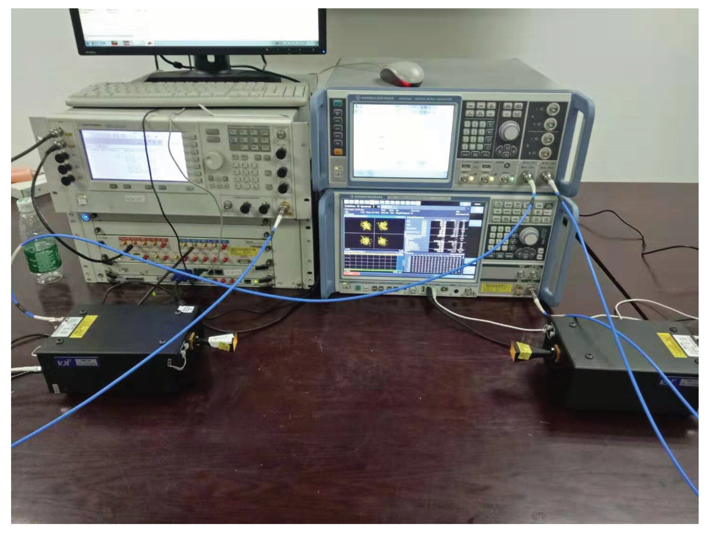
- We proposed and built the industry’s first commercial off-the-shelf (COTS) hardware-based high-frequency indoor millimeter wave channel sounding system based on time-domain correlation method, which could measure millimeter wave signals in the W-band.
- (2)
- We firstly proposed a data-driven supervised machine learning model for 6G indoor millimeter wave scene classification in the W-band.
- (3)
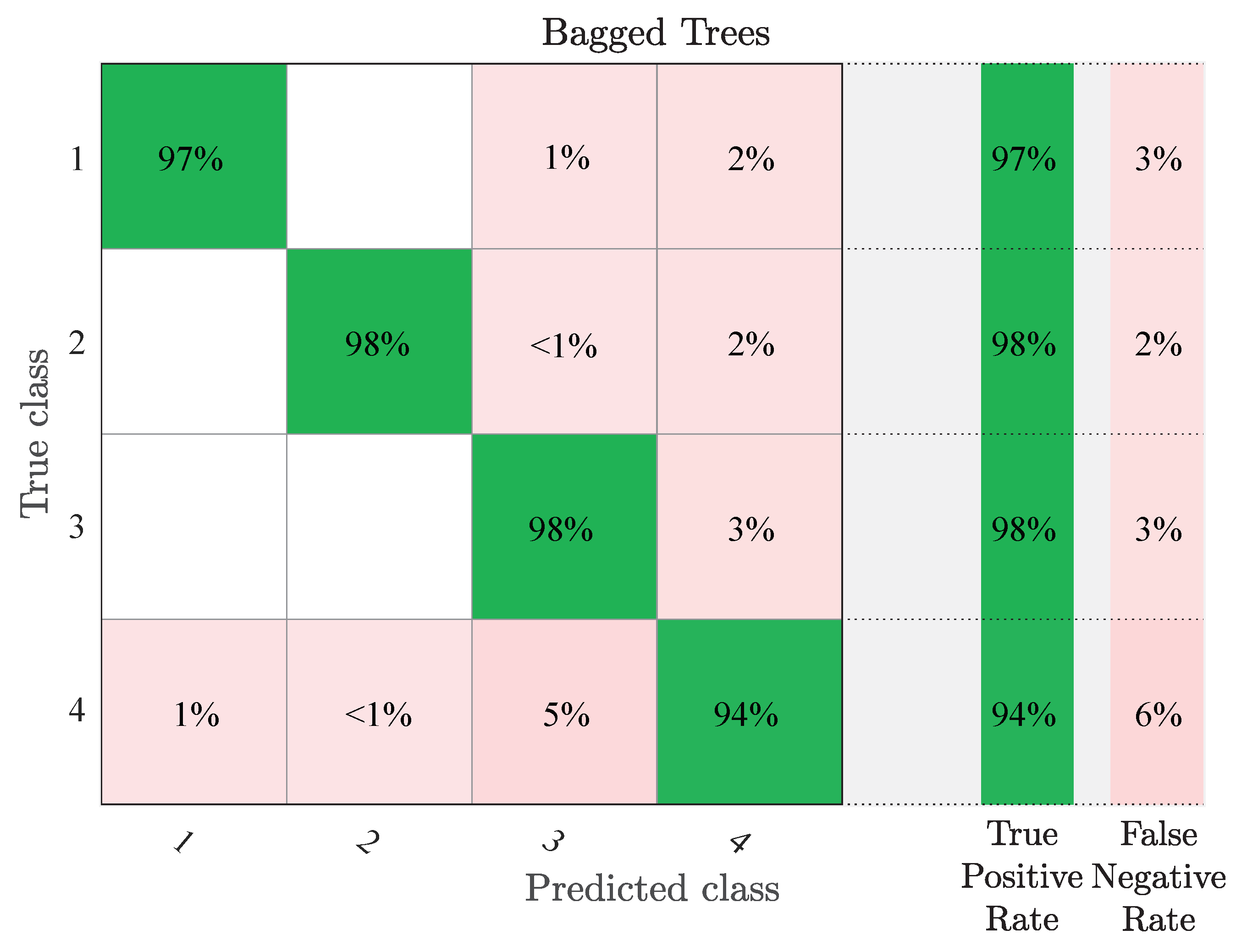
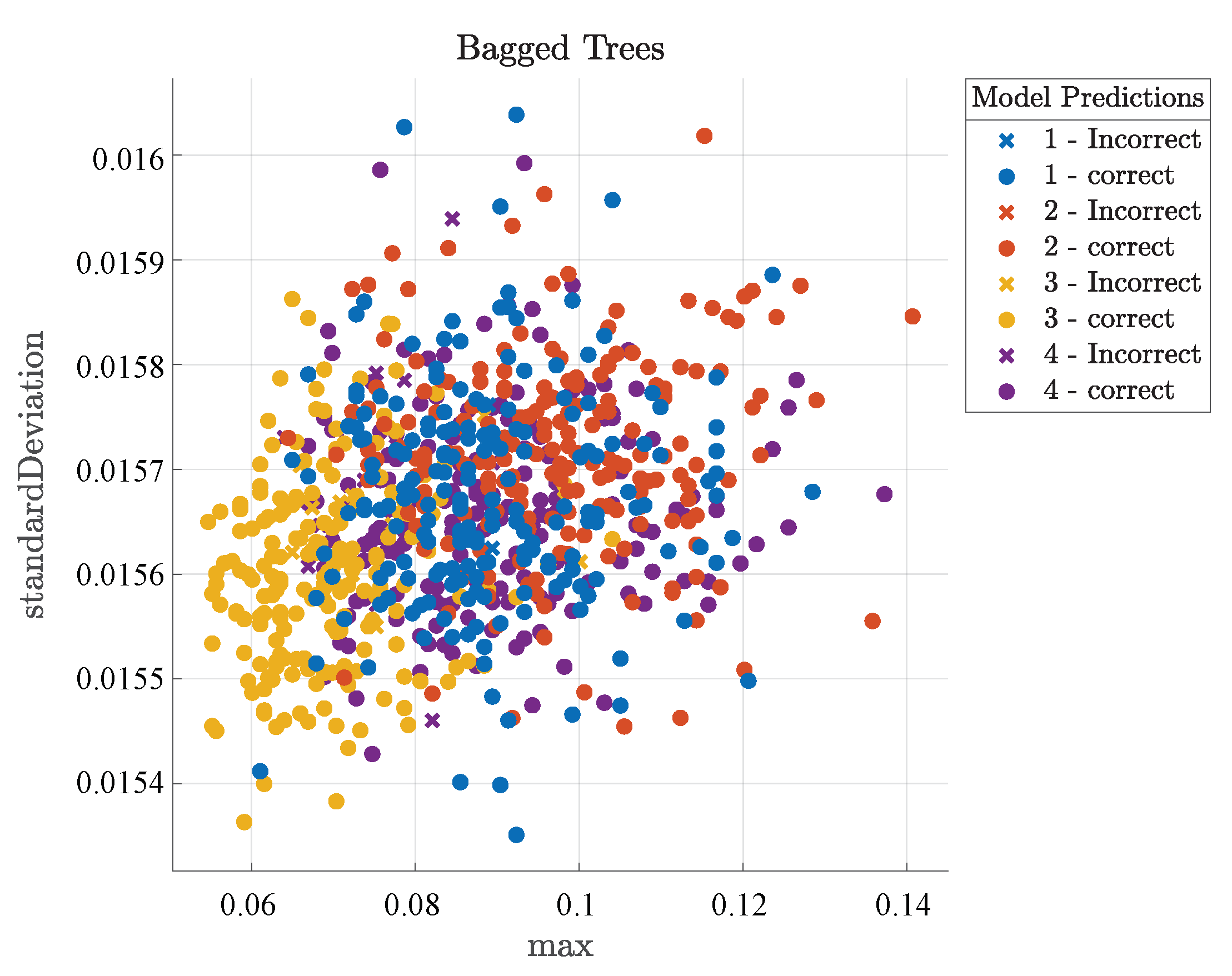
- The bagging classifier we firstly proposed is more efficient with 96.5% accuracy.
2. Materials and Methods
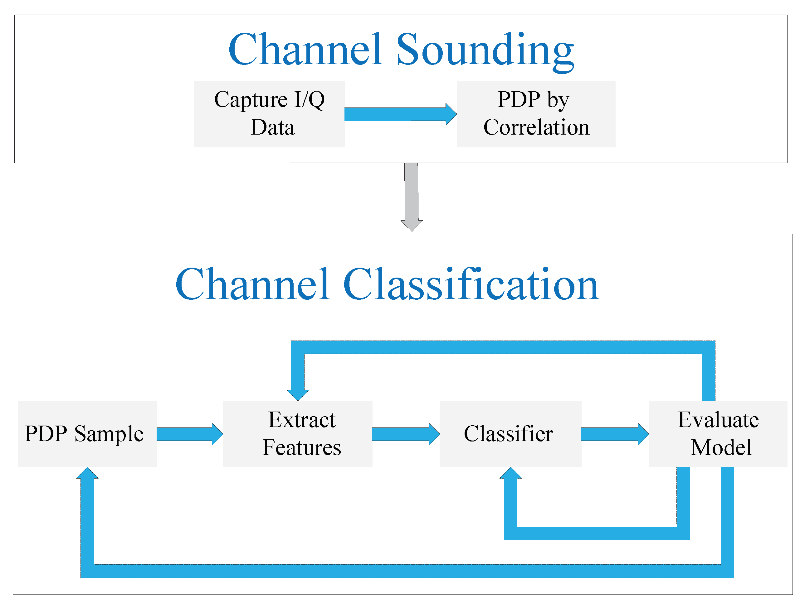
2.1. Channel Sounding and Classification
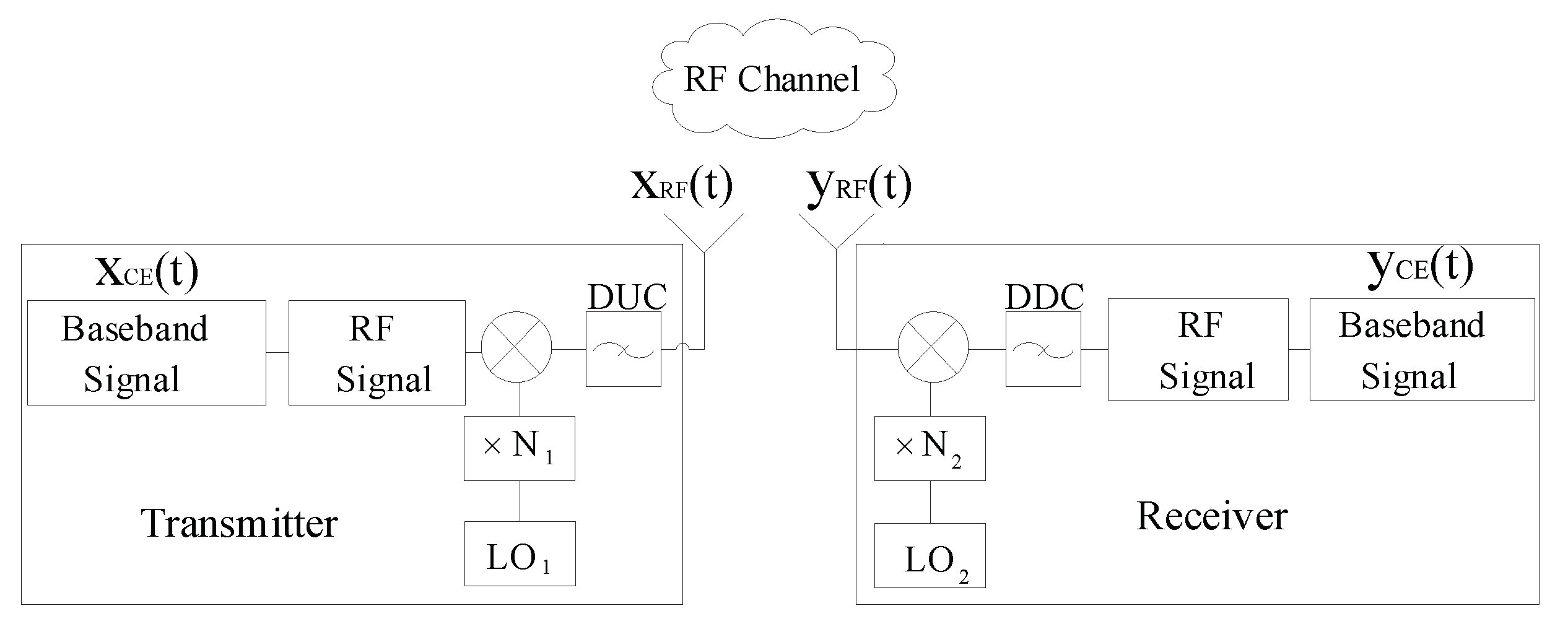
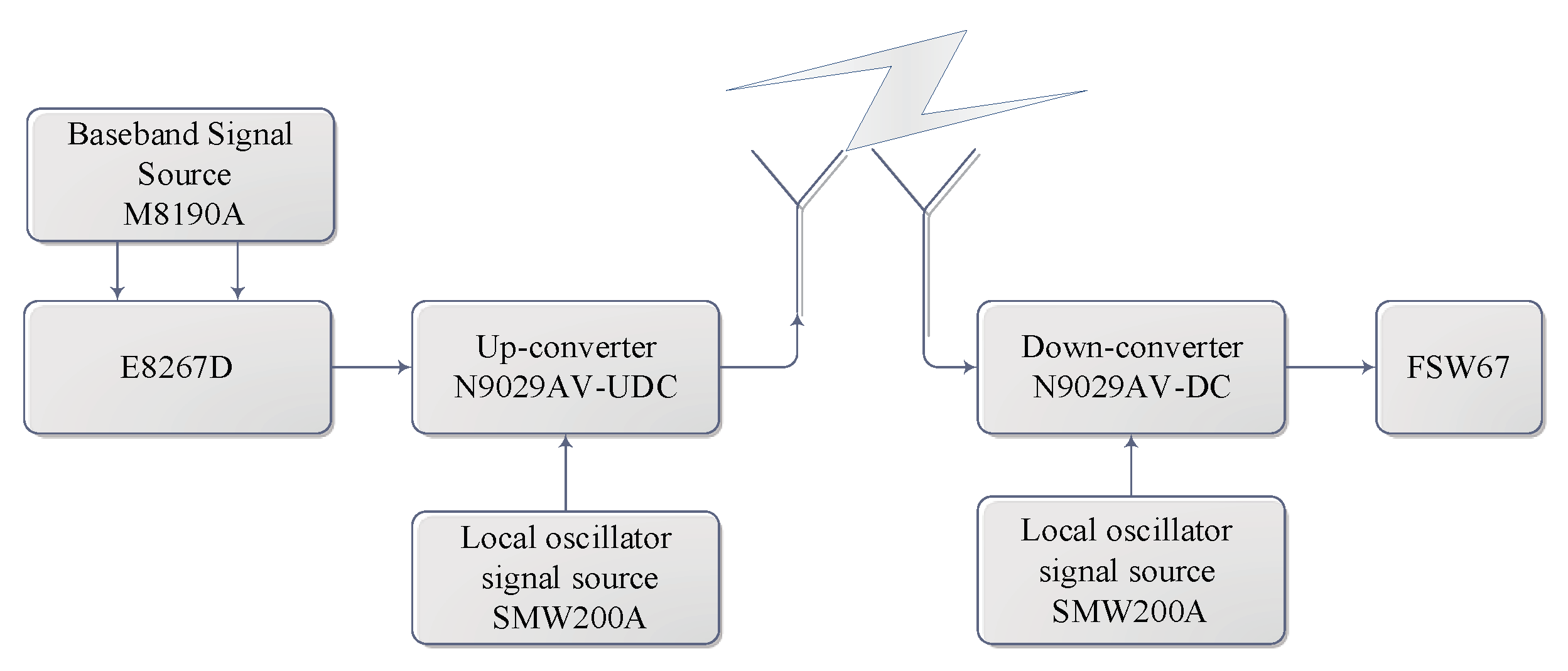
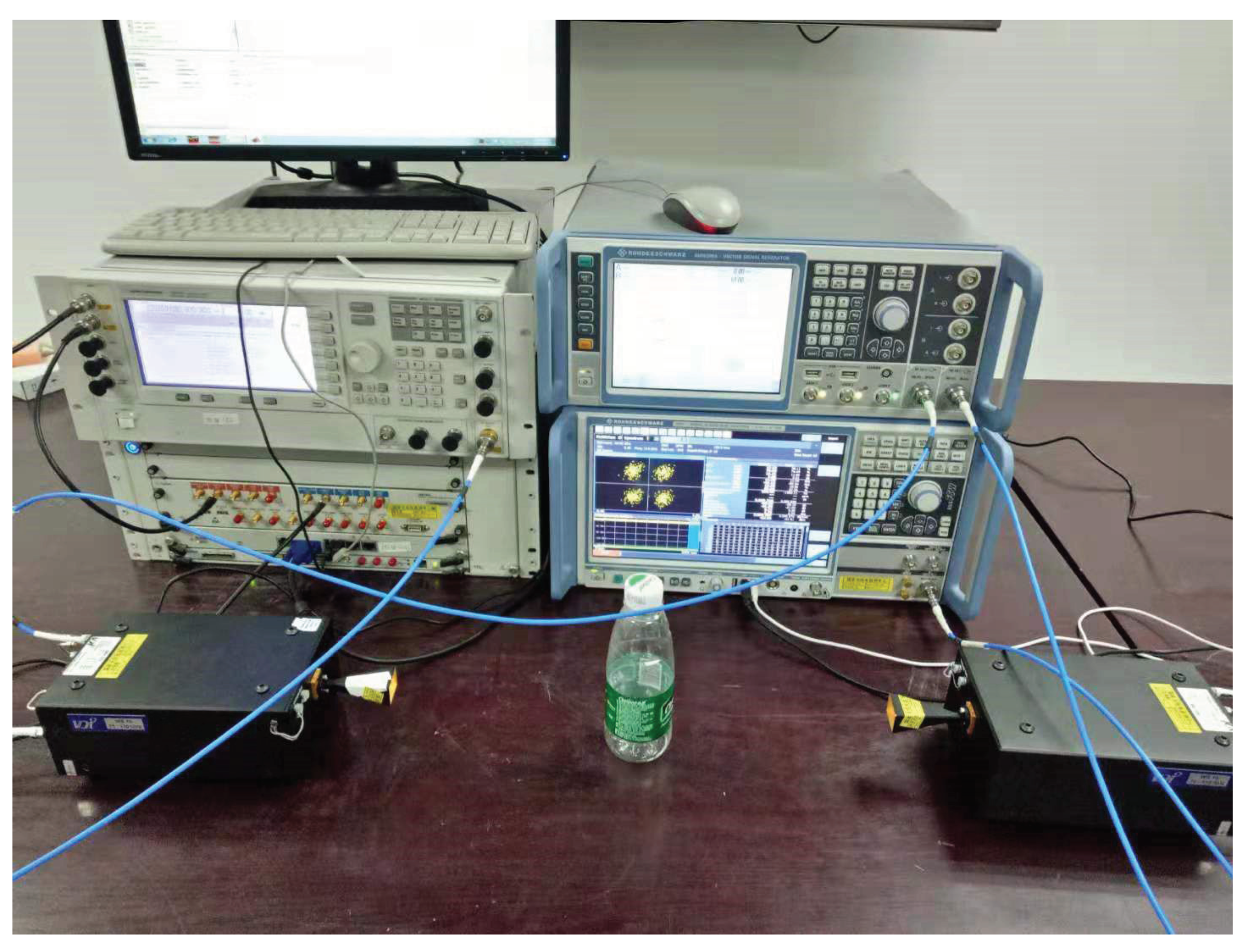
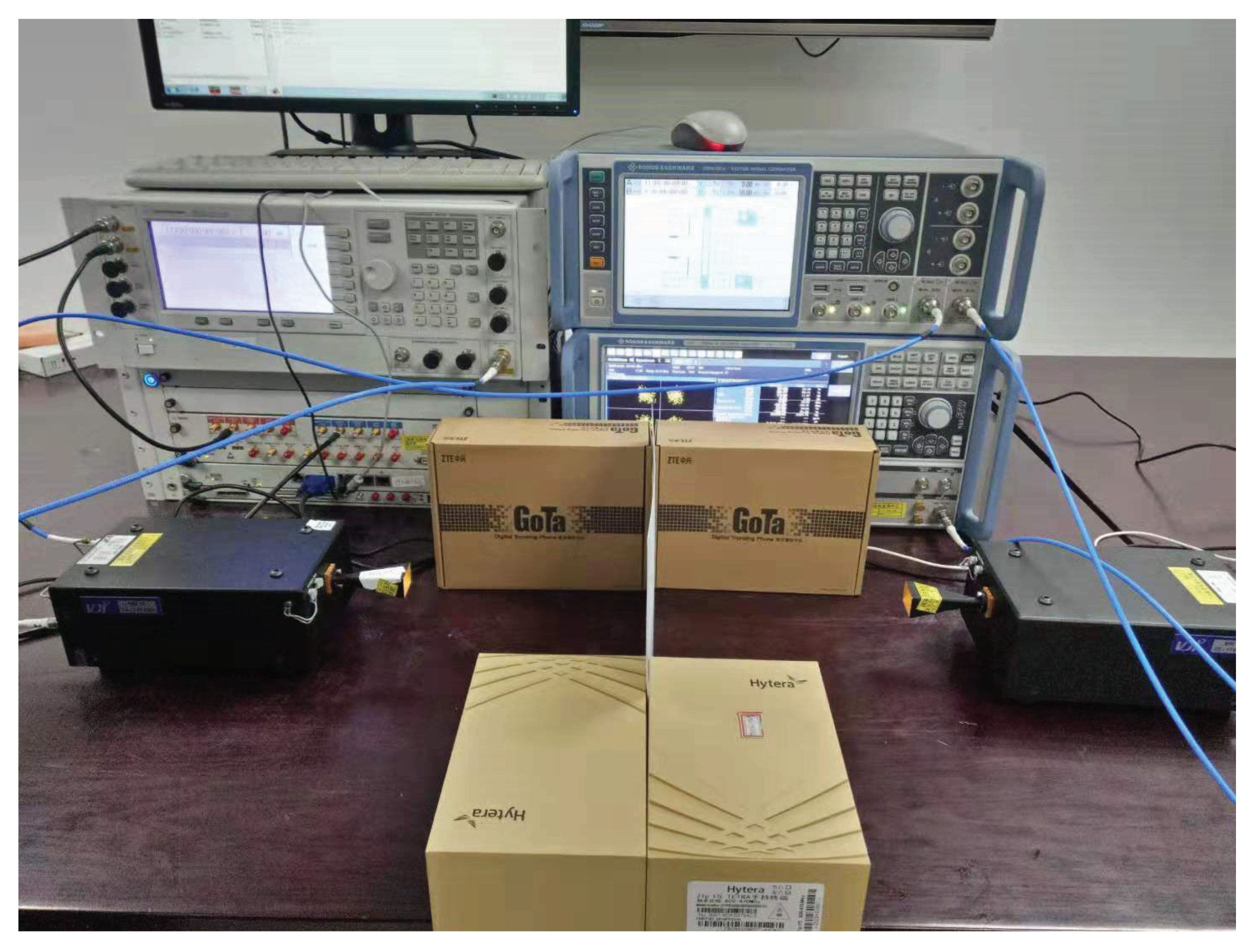
2.2. Channel Sounding
2.3. Channel Classification
2.3.1. Feature Extraction
2.3.2. Scene Classification Algorithms
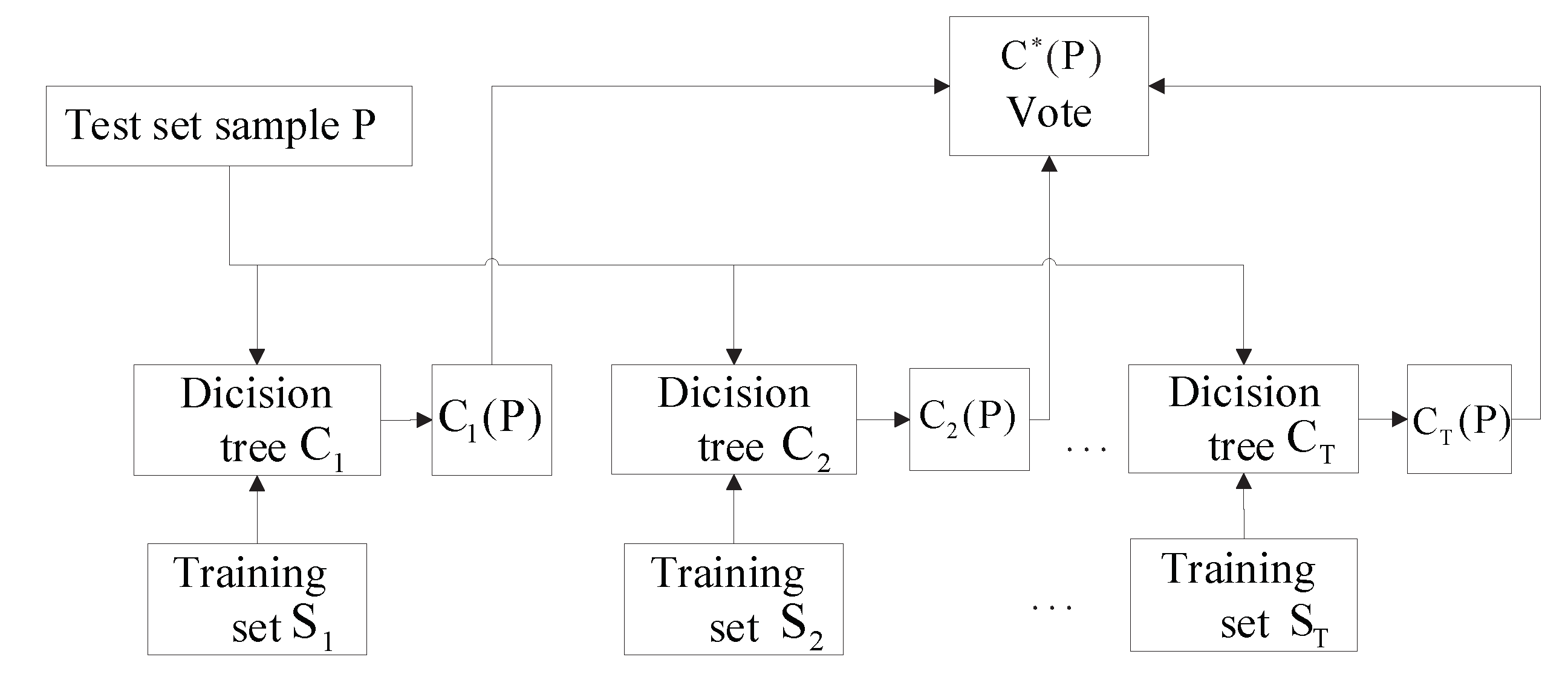
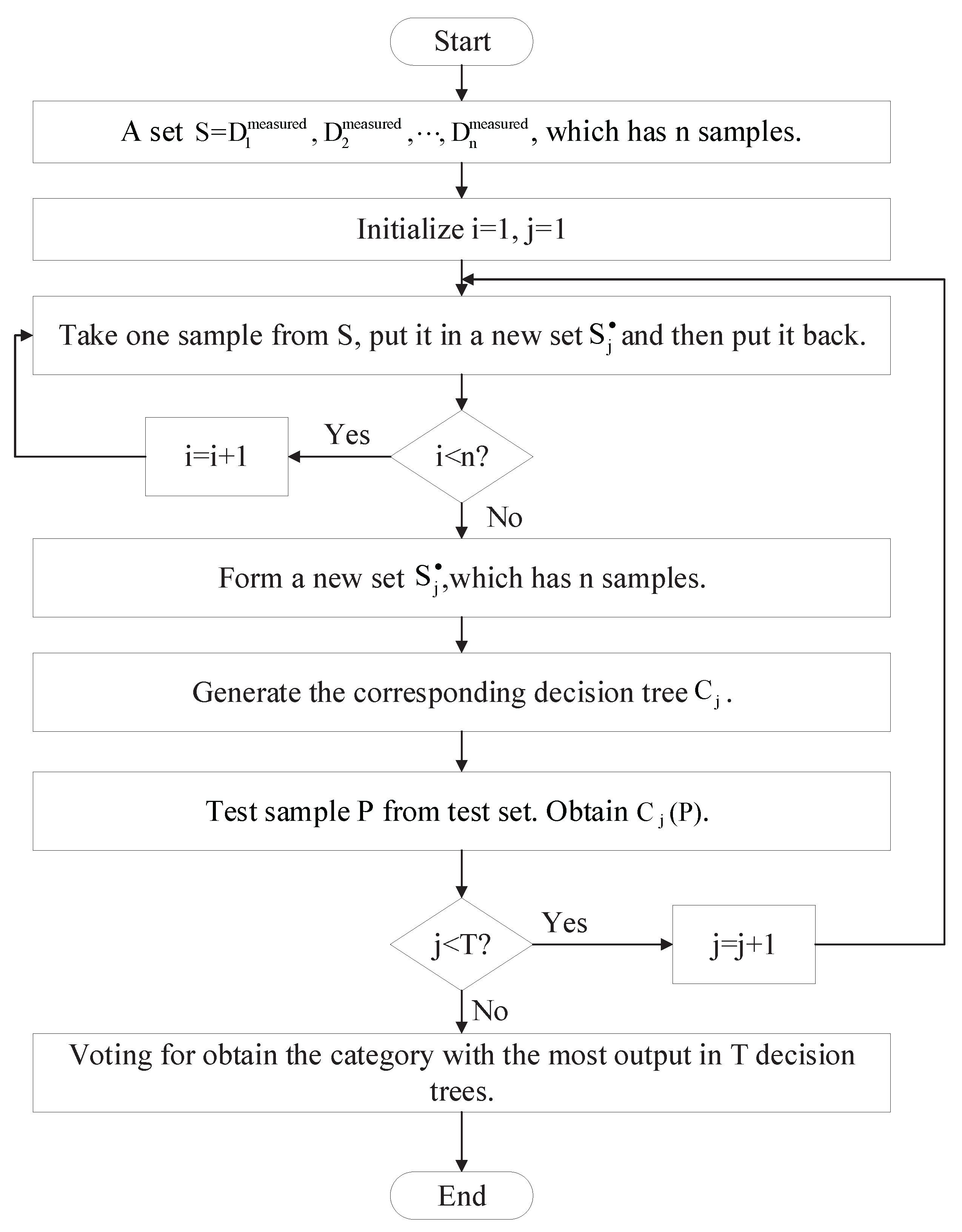
- i.
- Suppose that there are n samples in set , if we take one sample from set S every time, put it in a new set and then put it back, we will take a total of n times to form a new set . By resampling in this way, it can generate T training sets randomly.
- ii.
- Generate the corresponding decision tree by using each training set.
- iii.
- For the sample P from test set, each decision tree is used to test. Then obtain the corresponding category .
- iv.
- By voting, the category with the most output in T decision trees is taken as the category of sample P in the test set.
2.3.3. Method Verification and Evaluation
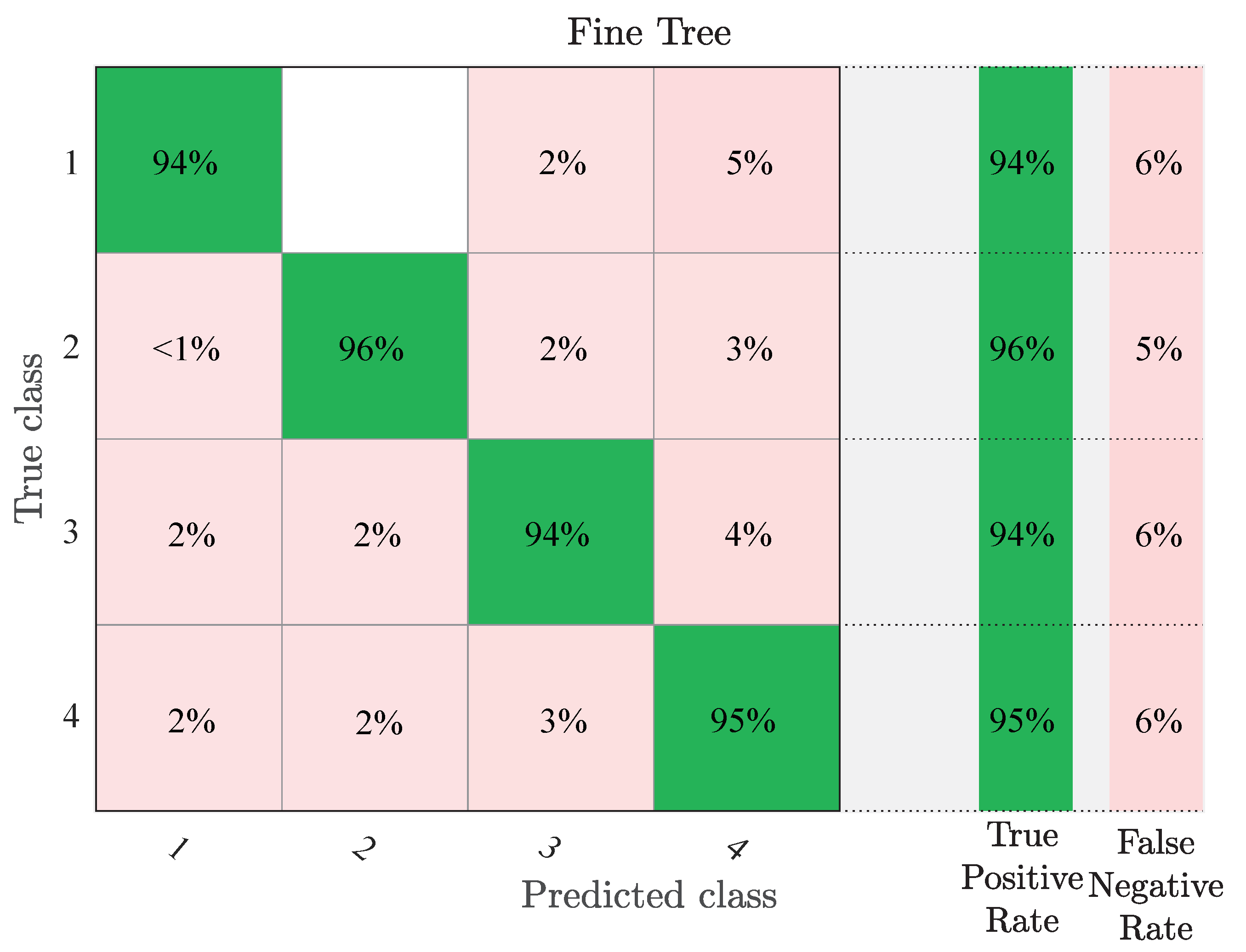
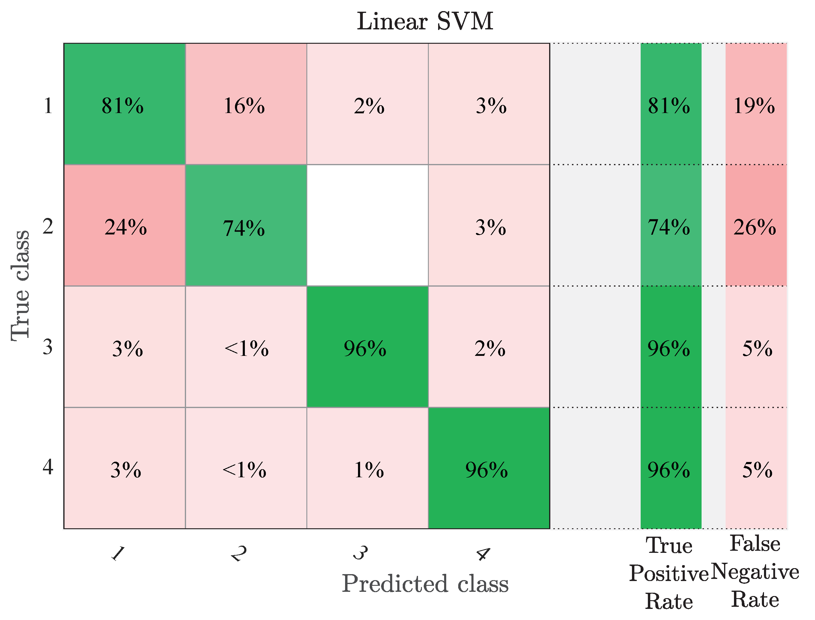
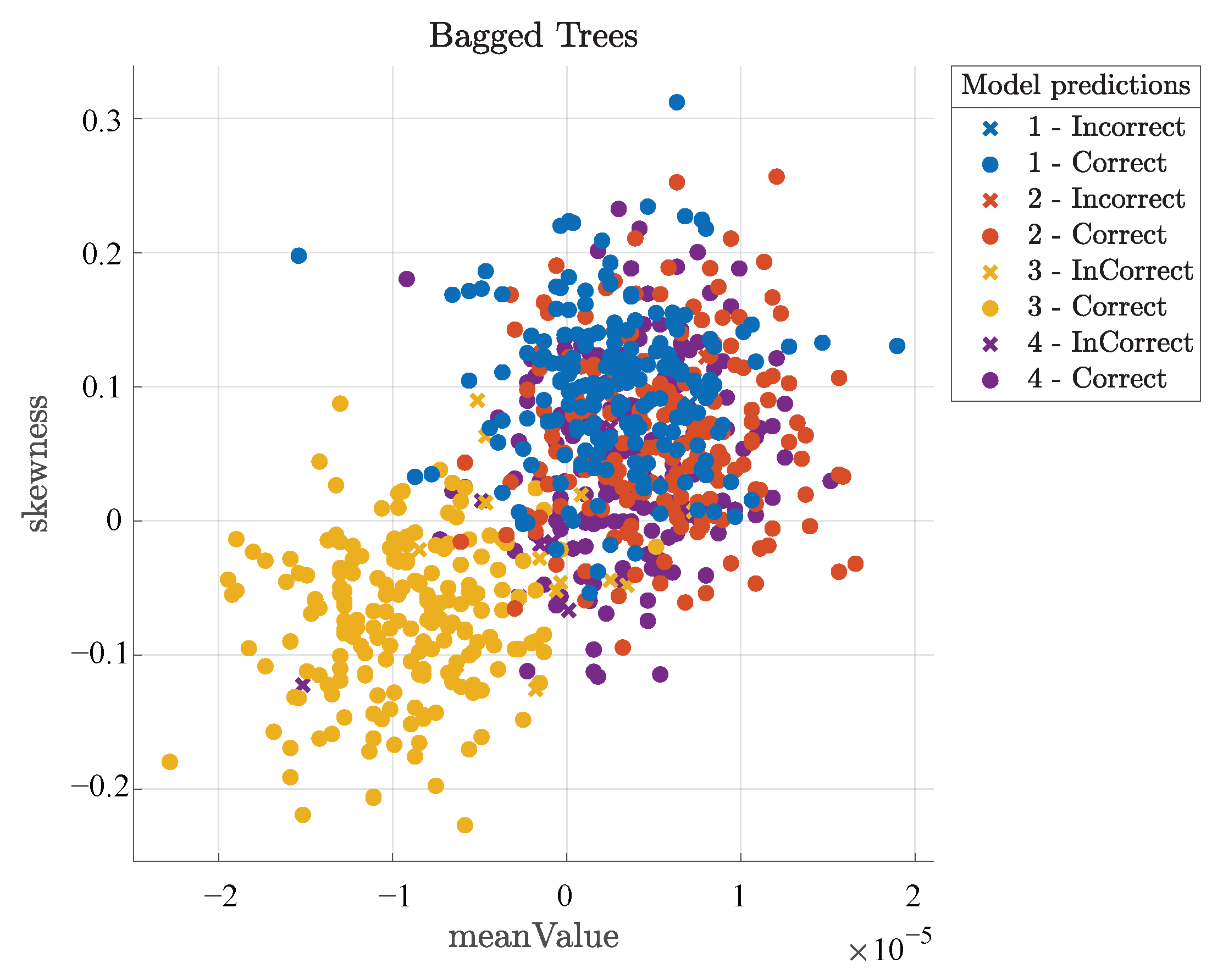
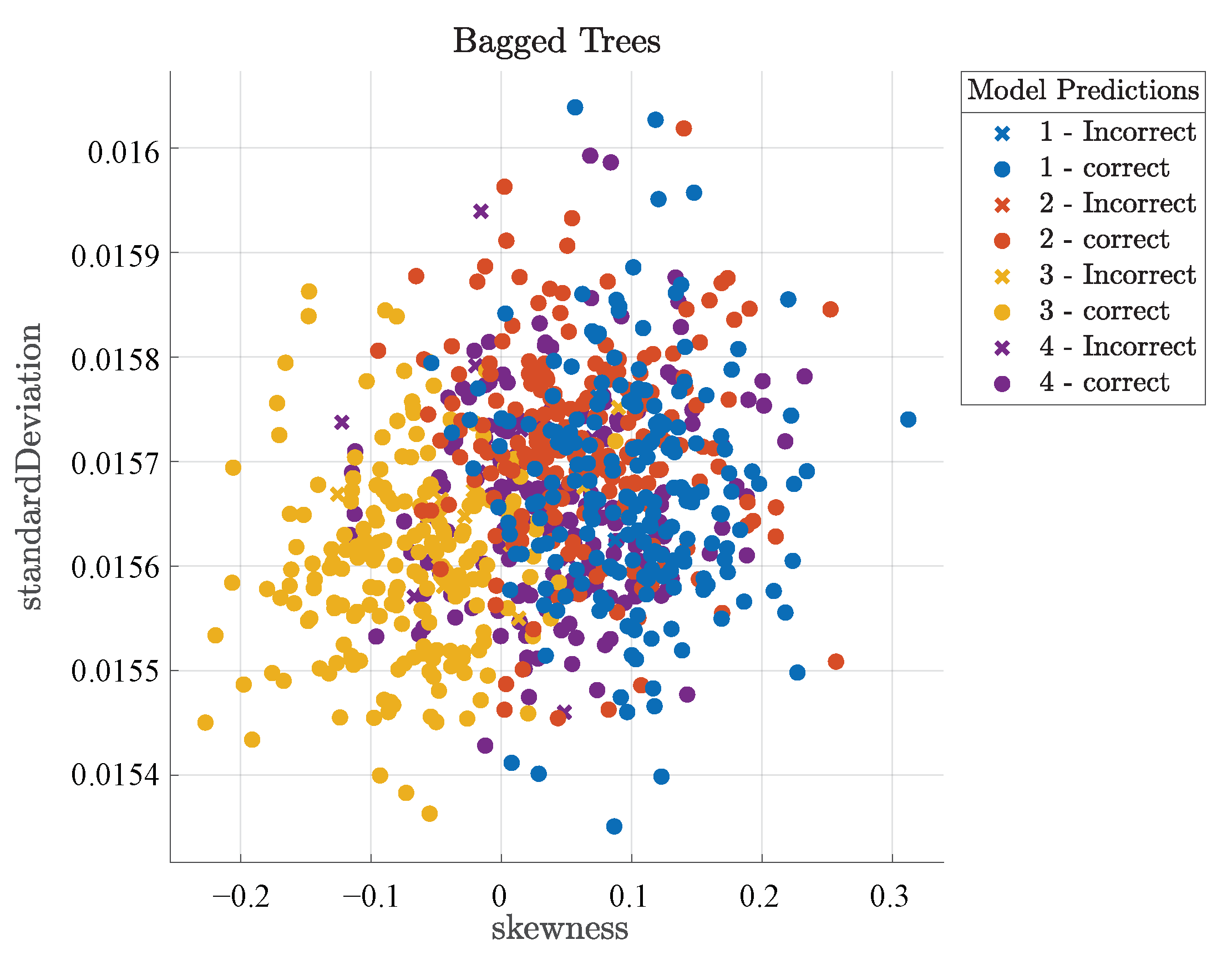
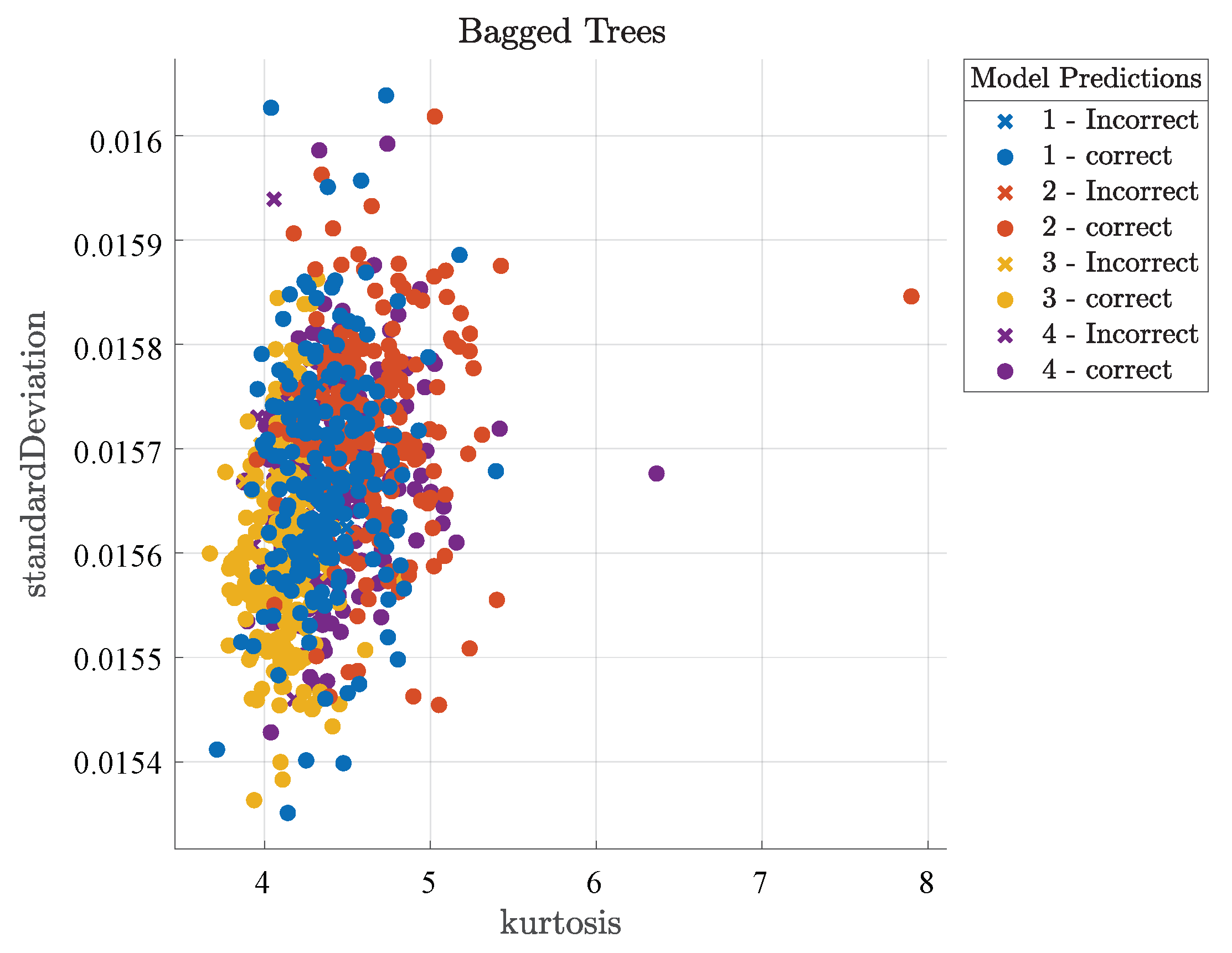
3. Results
4. Conclusions and Discussions
Author Contributions
Funding
Data Availability Statement
Acknowledgments
Conflicts of Interest
References
- Yong, N.; Yong, L.; Jin, D.; Li, S.; Vasilakos, A.V.J.W.N. A Survey of Millimeter Wave (mmWave) Communications for 5G: Opportunities and Challenges. Wirel. Netw. 2015, 21, 2657–2676. [Google Scholar]
- Rappaport, T.S.; Xing, Y.; Kanhere, O.; Ju, S.; Madanayake, A.; Mandal, S.; Alkhateeb, S.; Trichopoulos, G.C. Wireless Communications and Applications Above 100 GHz: Opportunities and Challenges for 6G and Beyond. IEEE Access 2019, 7, 78729–78757. [Google Scholar] [CrossRef]
- Sipal, V. Impact of the Wireless Channel on the Performance of Ultrawideband Communication Systems. Ph.D. Thesis, University of Oxford, Oxford, UK, 2012. [Google Scholar]
- Flikkema, P.G.; Johnson, S.G. A comparison of time- and frequency-domain wireless channel sounding techniques. In Proceedings of the Southeastcon 96 Bringing Together Education, Science and Technology, Tampa, FL, USA, 11–14 April 1996. [Google Scholar]
- Zhao, X.; Qi, W.; Shu, L.; Wang, M.; Sun, S. Wideband Millimeter-Wave Channel Characterization in an Open Office at 26 GHz. Wirel. Pers. Commun. 2017, 97, 5059–5075. [Google Scholar] [CrossRef]
- Hur, S.; Cho, Y.J.; Lee, J.A.; Kang, N.G.; Park, J.; Benn, H. Synchronous channel sounder using horn antenna and indoor measurements on 28 GHz. In Proceedings of the IEEE International Black Sea Conference on Communications and Networking, Odessa, Ukraine, 27–30 May 2014; pp. 83–87. [Google Scholar]
- Geng, S.; Liu, S.; Hong, W.; Zhao, X. Mm-wave 60 GHz indoor channel parameters and correlation properties. Dianbo Kexue Xuebao/Chin. J. Radio Sci. 2015, 30, 808–813. [Google Scholar]
- Maccartney, G.R.; Deng, S.; Sun, S.; Rappaport, T.S. Millimeter-Wave Human Blockage at 73 GHz with a Simple Double Knife-Edge Diffraction Model and Extension for Directional Antennas. In Proceedings of the 2016 IEEE 84th Vehicular Technology Conference (VTC-Fall), Montreal, QC, Canada, 18–21 September 2016. [Google Scholar]
- Zhang, J. The Interdisciplinary Research of Big Data and Wireless Channel: A Cluster-Nuclei Based Channel Model. China Commun. 2016, 13, 14–26. [Google Scholar] [CrossRef]
- Chen, X.; Liu, S.; Lu, J.; Fan, P.; Letaief, K.B. Smart Channel Sounder for 5G IoT: From Wireless Big Data to Active Communication. IEEE Access 2016, 4, 8888–8899. [Google Scholar] [CrossRef]
- Hayar, A.M.; Knopp, R.; Saadane, R. Subspace Analysis of Indoor UWB Channels. EURASIP J. Adv. Signal Process. 2005. [Google Scholar] [CrossRef]
- Sommerkorn, G.; Kaske, M.; Schneider, C.; Hafner, S.; Thoma, R. Full 3D MIMO channel sounding and characterization in an urban macro cell. In Proceedings of the General Assembly and Scientific Symposium, Beijing, China, 16–23 August 2014. [Google Scholar]
- Zhang, P.; Zhou, Y.; Sun, X.; Wang, H.; Terminal, C.J.M.C. Research on Techniques of Measurement and Modeling for 5G Millimeter Wave Channel. Mob. Commun. 2017. [Google Scholar] [CrossRef]
- Martinez-Ingles, M.-T.; Gaillot, D.P.; Pascual-Garcia, J.; Molina-Garcia-Pardo, J.-M.; Rodríguez, J.-V.; Rubio, L.; Juan-Llácer, L. Channel sounding and indoor radio channel characteristics in the W-band. EURASIP J. Wirel. Commun. Netw. 2016, 2016. [Google Scholar] [CrossRef]
- Smulders, P.; Wagemans, A.G. Frequency domain sounding of MM-wave indoor radio channels. In Proceedings of the 2nd IEEE International Conference on Universal Personal Communications, Ottawa, ON, Canada, 12–15 October 2002. [Google Scholar]
- Siamarou, A.G.; Al-Nuaimi, M. A Wideband Frequency-Domain Channel-Sounding System and Delay-Spread Measurements at the License-Free 57- to 64-GHz Band. IEEE Trans. Instrum. Meas. 2010, 59, 519–526. [Google Scholar] [CrossRef]
- Liu, Z.; Li, L.; Ye, P. Feature extraction of wireless mobile channel and the scene discrimination. J. Shanghai Norm. Univ. 2018. Available online: http://qktg.shnu.edu.cn/zrb/shsfqkszrben/ch/reader/view_abstract.aspx?file_no=20180204&flag=1 (accessed on 6 March 2021). [CrossRef]
- Chen, Y.; Zheng, Z.W.; Duan, H.; Zhang, M. The Extraction of the Fingerprints and Modeling in the Wireless Communication Channel. Wirel. Commun. Technol. 2017. [Google Scholar]
- Cal-Braz, J.A.; Matos, L.J.; Cataldo, E. The Relevance Vector Machine Applied to the Modeling of Wireless Channels. IEEE Trans. Antennas Propag. 2013, 61, 6157–6167. [Google Scholar] [CrossRef]
- Zhang, J.; Liu, L.; Fan, Y.; Zhuang, L.; Piao, Z. Wireless Channel Propagation Scenarios Identification: A Perspective of Machine Learning. IEEE Access 2020, 8, 47797–47806. [Google Scholar] [CrossRef]
- Lim, Y.G.; Cho, Y.J.; Min, S.S.; Kim, Y.; Valenzuela, R.A. Map-based Millimeter-Wave Channel Models: An Overview, Data for B5G Evaluation and Machine Learning. IEEE Wirel. Commun. 2020, 27, 54–62. [Google Scholar] [CrossRef]
- Yuan, J.; Ngo, H.Q.; Matthaiou, M. Machine Learning-Based Channel Prediction in Massive MIMO with Channel Aging. IEEE Wirel. Commun. 2020, 19, 2960–2973. [Google Scholar] [CrossRef]
- Wei, J.; Schotten, H.D. Deep Learning for Fading Channel Prediction. IEEE Open J. Commun. Soc. 2020, 1, 320–332. [Google Scholar]
- Ma, X.; Gao, Z. Data-Driven Deep Learning to Design Pilot and Channel Estimator for Massive MIMO. IEEE Trans. Veh. Technol. 2020, 69, 5677–5682. [Google Scholar] [CrossRef]
- Kurniawan, E.; Tan, P.H.; Sun, S.; Wang, Y.J.I. Machine Learning-based Channel-Type Identification for IEEE 802.11ac Link Adaptation. In Proceedings of the 2018 24th Asia-Pacific Conference on Communications (APCC), Ningbo, China, 12–14 November 2018. [Google Scholar]
- Ribeiro, C.; Gameiro, A. Direct Time-Domain Channel Impulse Response Estimation for OFDM-Based Systems. In Proceedings of the 2007 IEEE 66th Vehicular Technology Conference, Baltimore, MD, USA, 30 September–3 October 2007. [Google Scholar]
- Fontæn, F.P.; Espiæeira, P.M. Modeling the Wireless Propagation Channel:A Simulation Approach with MATLAB; John Wiley and Sons, Ltd.: Hoboken, NJ, USA, 2008. [Google Scholar]
- Goldsmith, A. Wireless Communications; Cambridge University Press: Cambridge, UK, 2007. [Google Scholar]
- Brandli, G.; Dick, M. Alternating-Current Fed Power Supply. U.S. Patent No 4,084,217, 1978. [Google Scholar]
- Horowitz, P.; Forster, J.; Linscott, I. The 8-million channel narrowband analyzer. In The Search for Extraterrestrial Life: Recent Developments; Cambridge University Press: Cambridge, UK, 1985. [Google Scholar]
- Sagnier, P.; Marraffa, L. Parametric Study of Thermal and Chemical Nonequilibrium Nozzle Flow. AIAA J. 2015, 29, 334–343. [Google Scholar] [CrossRef]
- Heiser, A.J. Private Communication. Private Commun. 2000, 8, 317–334. [Google Scholar]
- Smith, B. An approach to graphs of linear forms. Unpublished work. 1982. [Google Scholar]
- McKeeman, W.M. Representation Error for Real Numbers in Binary Computer Arithmetic. IEEE Trans. Electron. Comput. 1967, 5, 682–683. [Google Scholar] [CrossRef]
- Class, I.E. IEEE Criteria for Class IE Electric Systems for Nuclear Power Generating Stations. IEEE Std 308-1971 (Rev. IEEE Std 308-1980) 1970, PAS-89, 1365–1372. [Google Scholar] [CrossRef]
- United States of America Standards Institute. IEEE Standard Letter Symbols for Quantities Used in Electrical Science and Electrical Engineering; American Society of Mechanical Engineers: New York, NY, USA, 1984. [Google Scholar]
- Fardel, R.; Nagel, M.; Nüesch, F.; Lippert, T.; Wokaun, A. Fabrication of organic light-emitting diode pixels by laser-assisted forward transfer. Appl. Phys. Lett. 2007, 91, 61103. [Google Scholar] [CrossRef]
- Jing, Z.; Tansu, N. Optical Gain and Laser Characteristics of InGaN Quantum Wells on Ternary InGaN Substrates. IEEE Photonics J. 2013, 5, 2600111. [Google Scholar] [CrossRef]
- Azodolmolky, S.; Perello, J.; Angelou, M.; Agraz, F.; Velasco, L.; Spadaro, S.; Pointurier, Y.; Francescon, A.; Saradhi, C.V.; Kokkinos, P.; et al. Experimental Demonstration of an Impairment Aware Network Planning and Operation Tool for Transparent/Translucent Optical Networks. J. Light. Technol. 2011, 29, 439–448. [Google Scholar] [CrossRef]
- Cook, D.J.; Krishnan, N.C. Activity Learning: Discovering, Recognizing, and Predicting Human Behavior from Sensor Data; John Wiley and Sons, Ltd.: Hoboken, NJ, USA, 2015. [Google Scholar]
- Djosic, S.; Stojanovic, I.; Jovanovic, M.; Nikolic, T.; Djordjevic, G.L. Fingerprinting-Assisted UWB-based Localization Technique for Complex Indoor Environments. Expert Syst. Appl. 2021, 167, 114188. [Google Scholar] [CrossRef]
- Vongkulbhisal, J.; Chantaramolee, B.; Yan, Z.; Mohammed, W.S.; Letters, O.T. A fingerprinting—Based indoor localization system using intensity modulation of light emitting diodes. Microw. Opt. Technol. Lett. 2012, 54, 1218–1227. [Google Scholar] [CrossRef]
- Stella, M.; Russo, M.; Begušić, D. Location Determination in Indoor Environment based on RSS Fingerprinting and Artificial Neural Network. In Proceedings of the 2007 9th International Conference on Telecommunications, Zagreb, Croatia, 13–15 June 2007. [Google Scholar]
- Taok, A.; Kandil, N.; Affes, S. Neural Networks for Fingerprinting-Based Indoor Localization Using Ultra-Wideband. JCM 2009, 4, 267–275. [Google Scholar] [CrossRef]


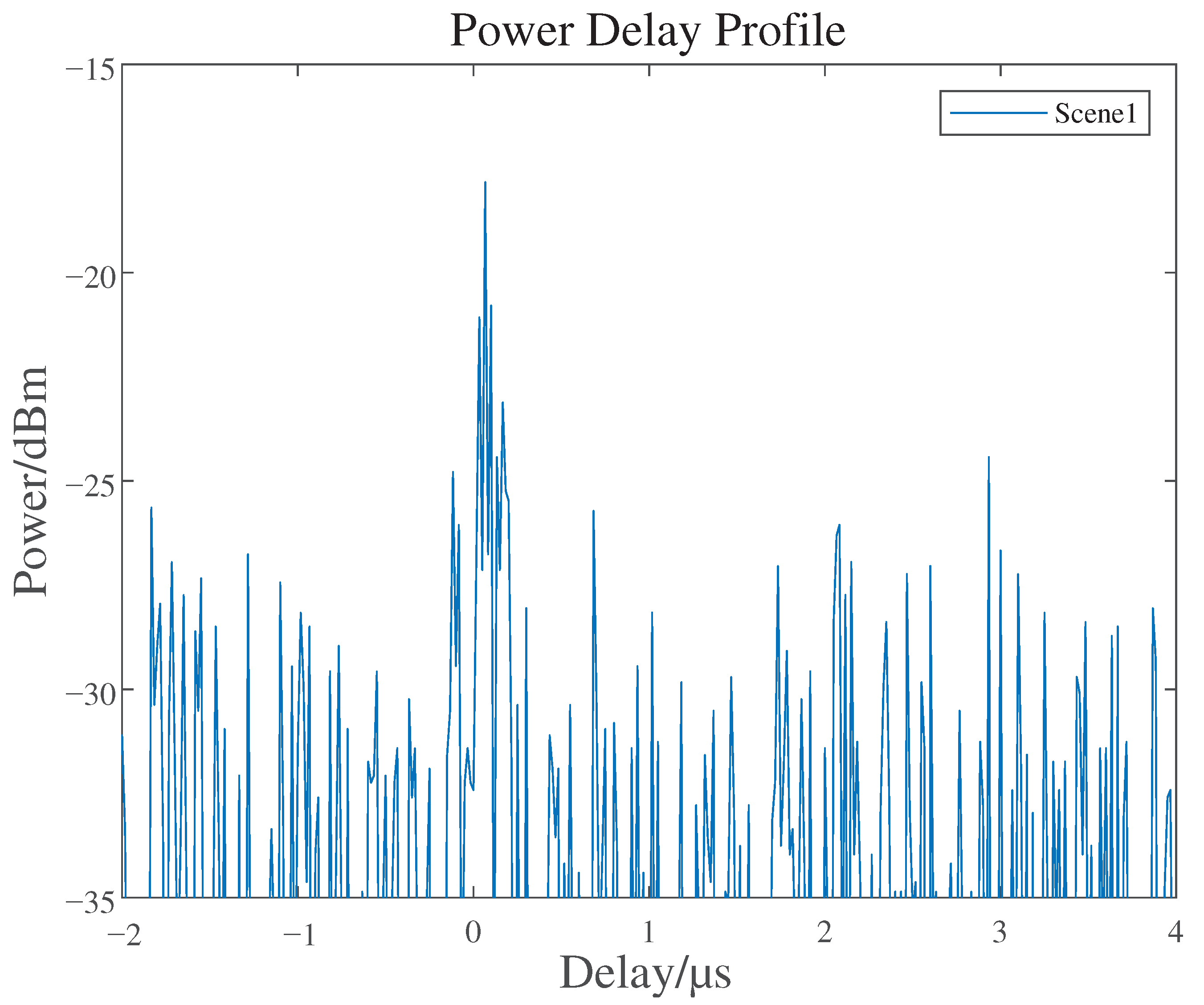
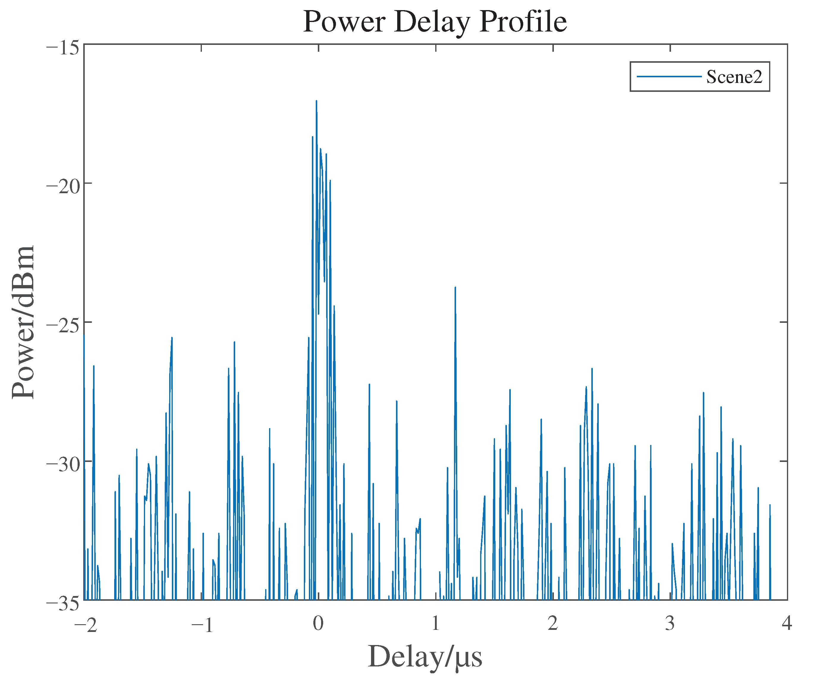
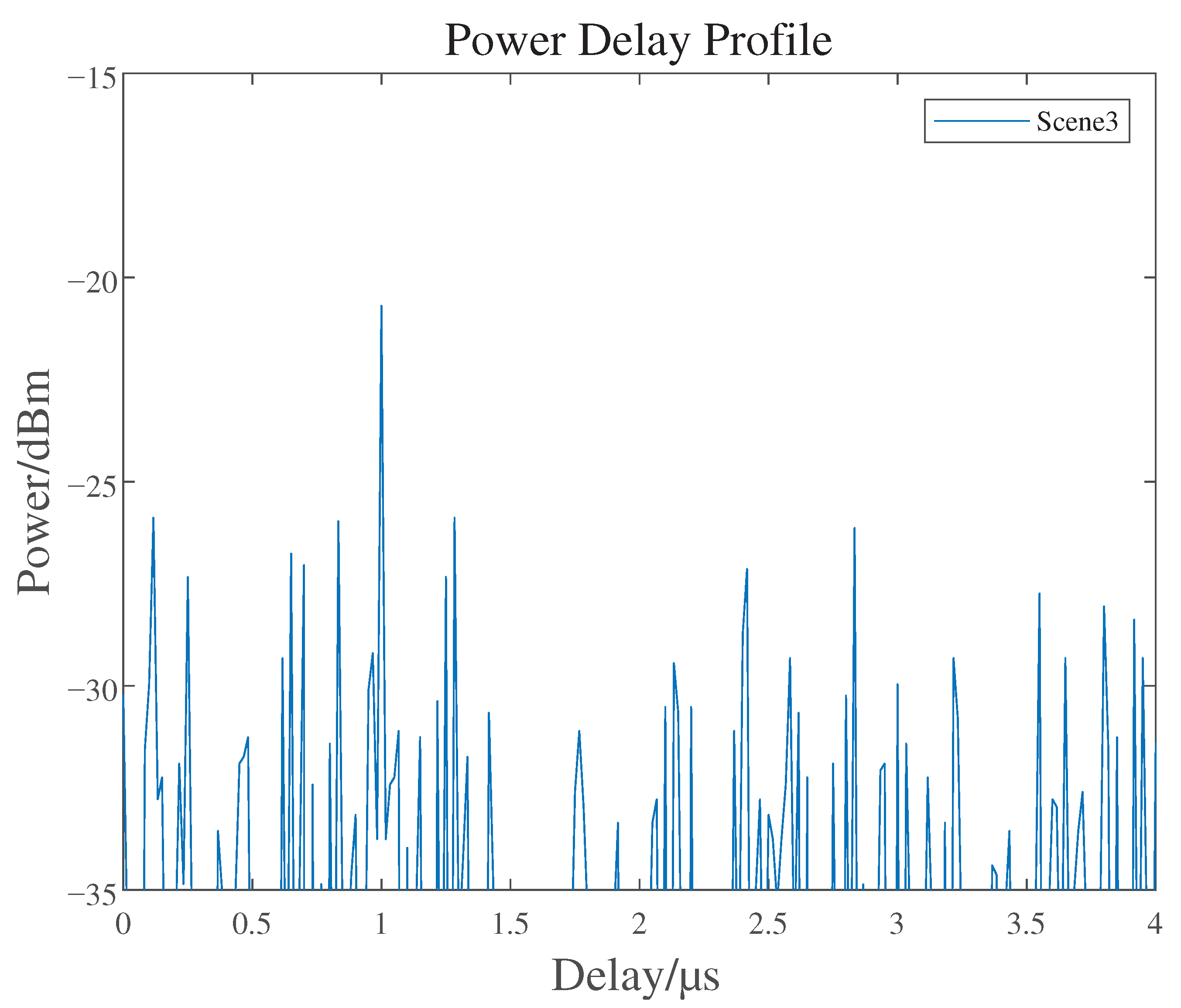
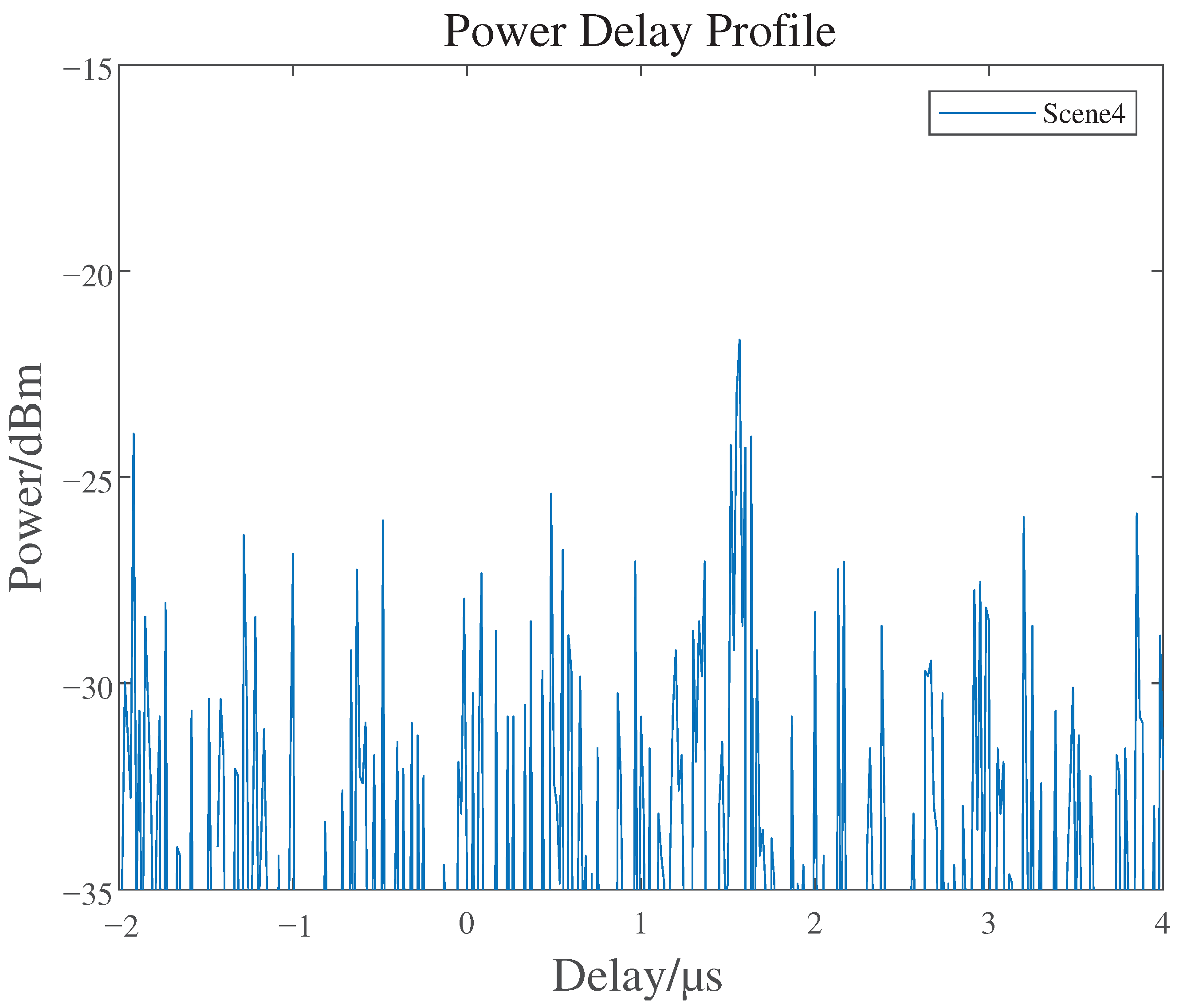
| Scene Number | Scene |
|---|---|
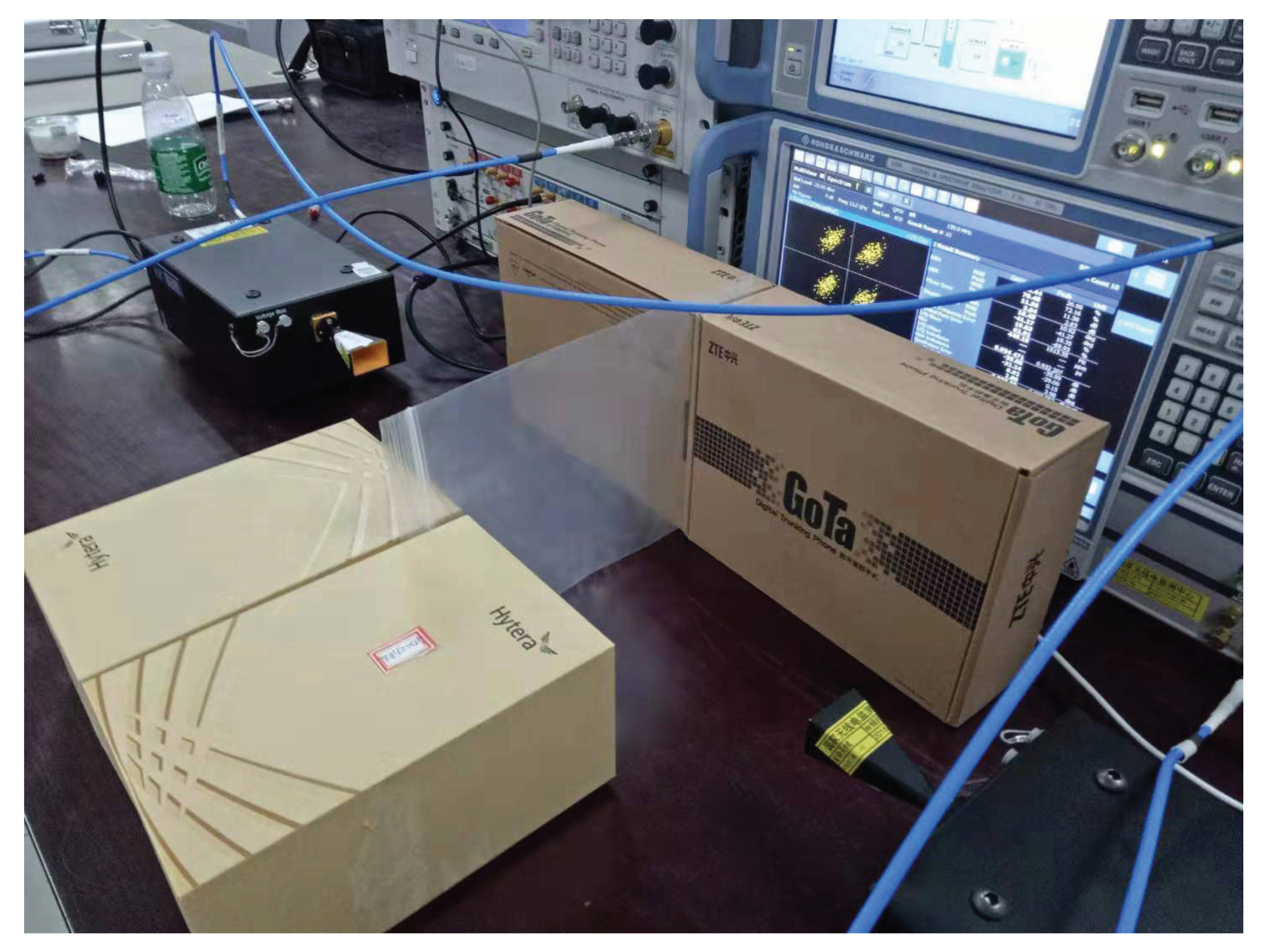
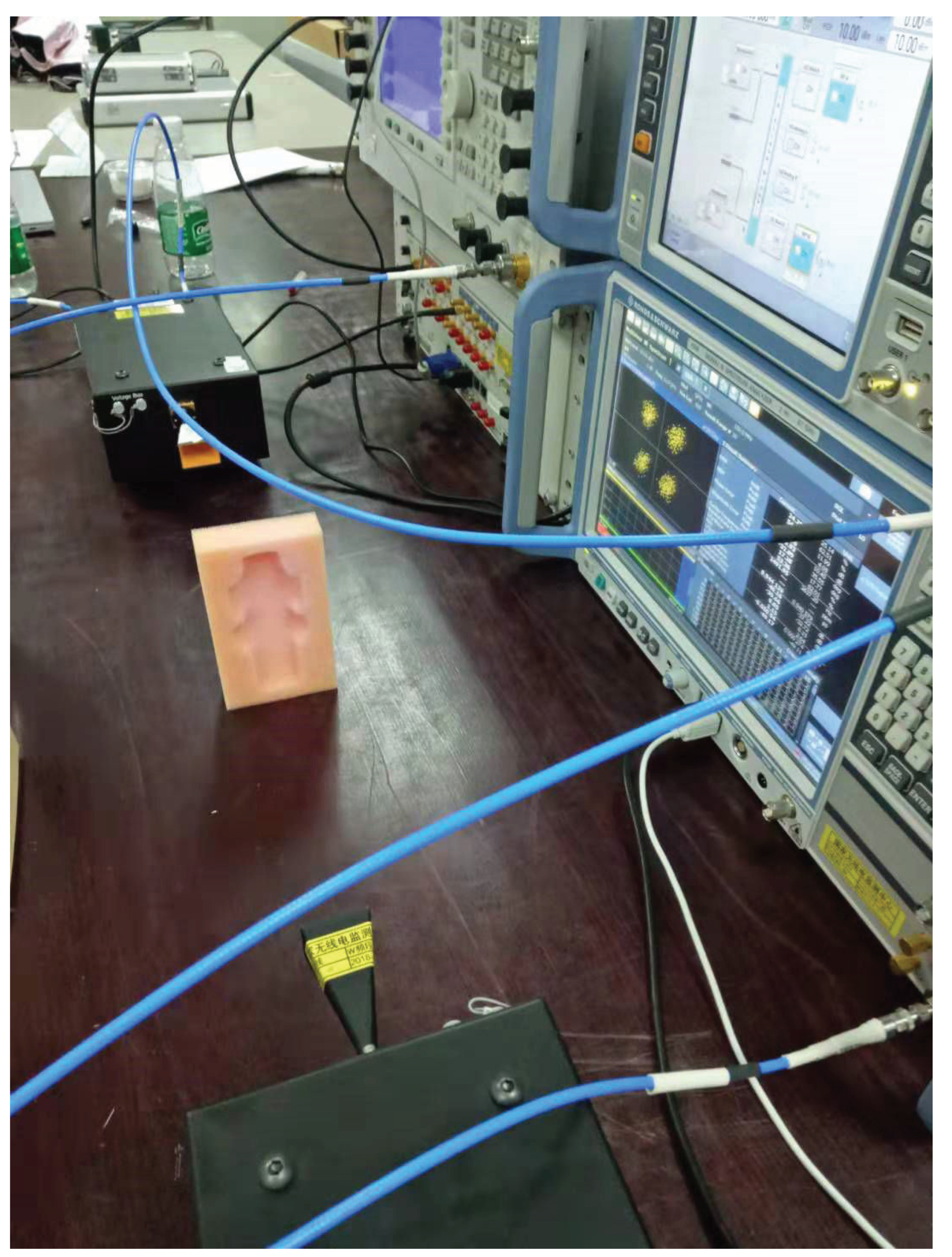
| 1 | An empty water bottle between the Tx and Rx antenna. |
| 2 | Two pieces of A4 paper between the Tx and Rx antenna. |
| 3 | A transparent plastic bag between the Tx and Rx antenna. |
| 4 | A sponge between the Tx and Rx antenna. |
| Scene Number | Delay/ | Power/dBm |
|---|---|---|
| 1 | 0.06667 | −17.82 |
| 2 | 0.01667 | −17.03 |
| 3 | 1 | −20.69 |
| 4 | 1.567 | −21.66 |
| Actual Positive | Actual Negative | |
|---|---|---|
| predicted positive | TP | FP |
| predicted negative | FN | TN |
| Classification Algorithm | Accuracy |
|---|---|
| Decision Tree | 94.3% |
| SVM | 86.4% |
| Bagging | 96.5% |
Publisher’s Note: MDPI stays neutral with regard to jurisdictional claims in published maps and institutional affiliations. |
© 2021 by the authors. Licensee MDPI, Basel, Switzerland. This article is an open access article distributed under the terms and conditions of the Creative Commons Attribution (CC BY) license (https://creativecommons.org/licenses/by/4.0/).
Share and Cite
Yin, L.; Yang, R.; Yao, Y. Channel Sounding and Scene Classification of Indoor 6G Millimeter Wave Channel Based on Machine Learning. Electronics 2021, 10, 843. https://doi.org/10.3390/electronics10070843
Yin L, Yang R, Yao Y. Channel Sounding and Scene Classification of Indoor 6G Millimeter Wave Channel Based on Machine Learning. Electronics. 2021; 10(7):843. https://doi.org/10.3390/electronics10070843
Chicago/Turabian StyleYin, Liang, Ruonan Yang, and Yuliang Yao. 2021. "Channel Sounding and Scene Classification of Indoor 6G Millimeter Wave Channel Based on Machine Learning" Electronics 10, no. 7: 843. https://doi.org/10.3390/electronics10070843
APA StyleYin, L., Yang, R., & Yao, Y. (2021). Channel Sounding and Scene Classification of Indoor 6G Millimeter Wave Channel Based on Machine Learning. Electronics, 10(7), 843. https://doi.org/10.3390/electronics10070843