Article

Investigating the Effects of Training Set Synthesis for Audio Segmentation of Radio Broadcast

Interdisciplinary Centre for Computer Music Research, University of Plymouth, Plymouth PL4 8AA, UK
*
Author to whom correspondence should be addressed.
Electronics 2021, 10(7), 827; https://doi.org/10.3390/electronics10070827
Submission received: 26 February 2021 / Revised: 26 March 2021 / Accepted: 28 March 2021 / Published: 31 March 2021
(This article belongs to the Special Issue Machine Learning Applied to Music/Audio Signal Processing)

Abstract

:
Music and speech detection provides us valuable information regarding the nature of content in broadcast audio. It helps detect acoustic regions that contain speech, voice over music, only music, or silence. In recent years, there have been developments in machine learning algorithms to accomplish this task. However, broadcast audio is generally well-mixed and copyrighted, which makes it challenging to share across research groups. In this study, we address the challenges encountered in automatically synthesising data that resembles a radio broadcast. Firstly, we compare state-of-the-art neural network architectures such as CNN, GRU, LSTM, TCN, and CRNN. Later, we investigate how audio ducking of background music impacts the precision and recall of the machine learning algorithm. Thirdly, we examine how the quantity of synthetic training data impacts the results. Finally, we evaluate the effectiveness of synthesised, real-world, and combined approaches for training models, to understand if the synthetic data presents any additional value. Amongst the network architectures, CRNN was the best performing network. Results also show that the minimum level of audio ducking preferred by the machine learning algorithm was similar to that of human listeners. After testing our model on in-house and public datasets, we observe that our proposed synthesis technique outperforms real-world data in some cases and serves as a promising alternative.

1. Introduction

Audio segmentation is an event-detection task that identifies audio events and their respective boundaries. It divides an audio signal into sections based on the composite acoustic classes such as speech, singing voice, and environmental sounds. Segmentation of audio helps us develop metadata regarding its content, which often serves as a preprocessing step for a bigger task like speech and lyrics transcription, content recognition, and indexing. Audio segmentation of radio and television programmes has been highly relevant in the literature to detect sections of speech, music, or both [1].
High regions of acoustic change can be either detected by using a distance-metric or modelled as a supervised learning task [2]. Distance-based segmentation directly detects regions of high acoustic changes in an unsupervised way. A distance metric such as Euclidean distance [3], Bayesian information criterion (BIC) [4], or generalized likelihood ratio (GLR) [5] is computed to detect peaks of acoustic change. These peaks are associated with the transition from one acoustic class to another.
Segmentation-by-classification is a supervised learning method that divides audio into small frames, typically in the range of 10 to 25 ms. These audio frames are individually classified as music or speech and thus detect the boundaries of audio events. This technique has gained popularity after deep learning was investigated for audio segmentation.
Many studies have explored novel algorithms and neural network architectures to improve the performance of audio segmentation. However, there has been less focus on the availability of data to train these machine learning models. There are many openly available datasets that contain separate audio files of music and speech. For example, LibriSpeech contains a vast number of speech examples and GTZAN genre recognition dataset has many music examples. However, broadcast audio is well-mixed by engineers and it contains speech over background music or gradual fade in and fade out of music. Over the years, researchers have trained their models on broadcast audio and unfortunately cannot share their datasets due to copyright issues [6,7,8]. This hinders the reproducibility of research.
Among datasets for audio segmentation, MuSpeak [9] was an example dataset provided by the Music Information Retrieval Evaluation eXchange (MIREX) 2018 music and speech detection competition (https://music-ir.org/mirex/wiki/2018:Music_and/or_Speech_Detection, accessed on 26 February 2021). It is an openly available dataset that contains approximately 5 h of broadcast audio with annotations of music and speech. Moreover, a dataset called Open Broadcast Media Audio from TV (OpenBMAT) [10] comprises 27.4 h of audio, with annotations for the relative loudness of music, but not speech. To train models for segmentation, in-house datasets are generally annotated by authors or outsourced to annotators. For instance, Schlüter et al. [6] paid students to annotate 42 h of radio broadcast. OpenBMAT was cross-annotated by three individuals.
Annotating broadcast audio takes up a lot of time. The annotator needs to precisely detect transition points, silences between speech, and music smoothly fading in and out. Therefore, annotating an hour of audio usually ends up taking four to five hours. For example, each annotator of OpenBMAT took approximately 130 h [10]. Furthermore, the presence of background music at very low volumes becomes a subjective task with differences amongst annotators. Hence, audio is annotated by multiple individuals, making the process expensive and laborious.
In this paper, we investigate the challenges involved in automatically mixing audio content that would resemble radio data. The speech and music files used by the data synthesis procedure are restricted to openly available datasets to encourage reproducibility. We replicate the process of a mixing engineer by investigating fade curves and audio ducking. The literature comprises many mixing principles adopted by radio stations, such as sufficient loudness difference between speech and background music to make the speech intelligible. We evaluate and implement these mixing principles and choose optimal parameters for our data synthesis algorithm.
Our initial findings using this data synthesis procedure was accepted as a conference paper in IEEE ICASSP [11]. However, the novel contributions of this journal paper are: (1) compare state-of-the-art neural network architectures for audio segmentation, (2) investigate how the loudness difference between speech and background music influences the performance of segmentation, (3) examine how the size of the training set improves performance (4) compare real-world training sets and synthetic training sets. The implementation, code, and pretrained models associated with this study is openly available in this GitHub repository (https://github.com/satvik-venkatesh/train-synth-audio-seg/, accessed on 26 February 2021).

Paper Structure

Section 2 explains the procedure to artificially synthesise radio data. In Section 3, we present the methods that are common to all experiments. We conduct four different experiments in Section 4, Section 5, Section 6 and Section 7. For clarity, we explain the experimental set-up and results for each experiment within the section itself. Section 4 compares state-of-the-art neural network architectures. Subsequently, in Section 5, we investigate the effect of loudness difference between speech and background music. Section 6 evaluates how the size of the synthetic training set impacts performance. Finally, in Section 7, we compare machine learning models trained on synthetic and real-world data.
Please note that the results presented in Section 4, Section 5 and Section 6 were on both our validation set and test set. We present the results on the validation set because we are optimising model settings and fine-tuning parameters for data synthesis. All our decisions were informed by only the validation set because we did not want to influence the test results of the main experiment in Section 7. However, for Section 4, Section 5 and Section 6, we also present the results on the test set to ensure that we are not overfitting the validation set. The results for the final experiment in Section 7 were only on the test set, which demonstrates the robustness of our data synthesis procedure.

2. Data Synthesis

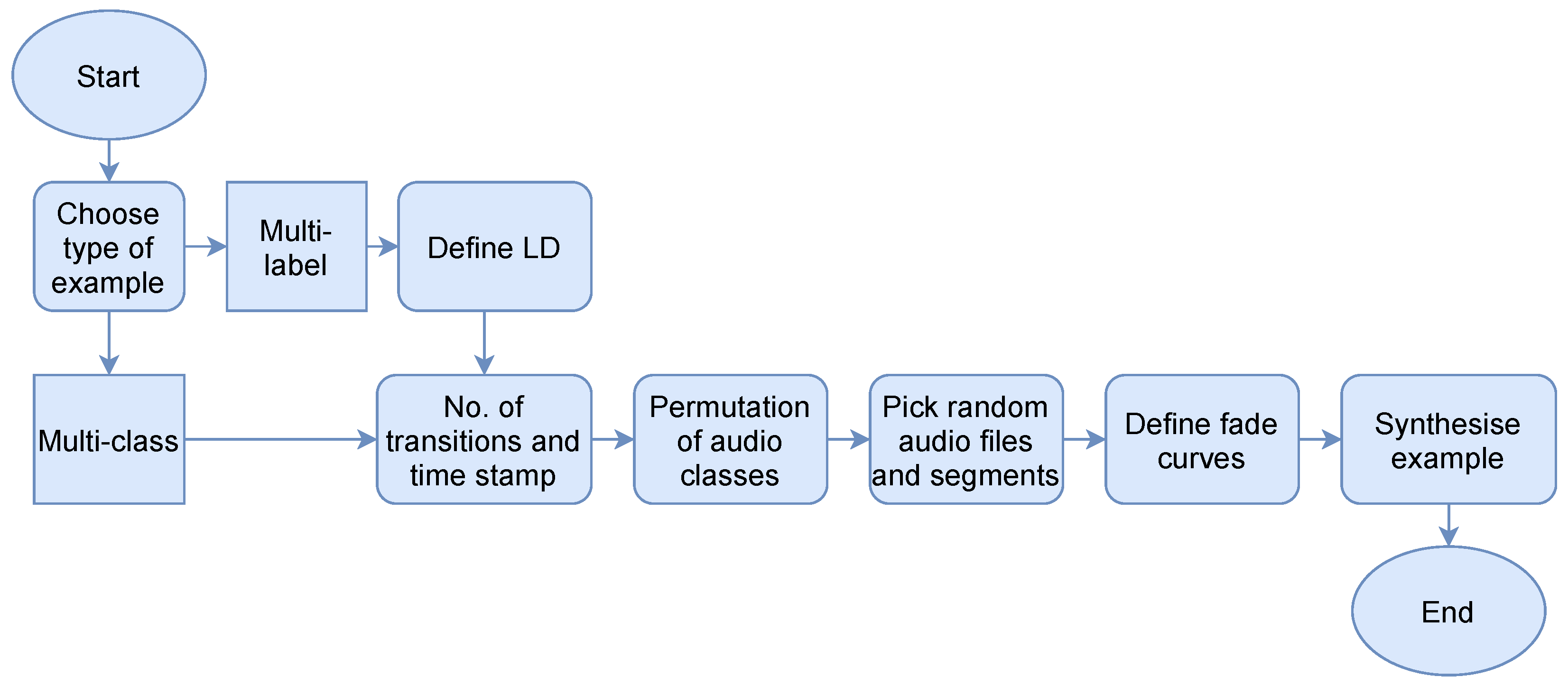
2.1. Synthetic Examples

We considered four combinations of audio classes which commonly occur in radio programmes—speech, music, speech over music, or other. Another common feature in radio programmes is the smooth transition from one audio class to another. We synthesised audio examples with a fixed duration of 8 s. We felt that 8 s was long enough to clearly identify the audio class and capture transitions that might occur between one audio class to another. For clarity, we categorised the examples into two types—(1) Multi-class examples and (2) Multi-label examples. The former focuses on audio where either music, speech, or noise can occur. There is no simultaneous occurrence of two acoustic classes. In multi-label examples, we specifically focus on audio with speech over background music.

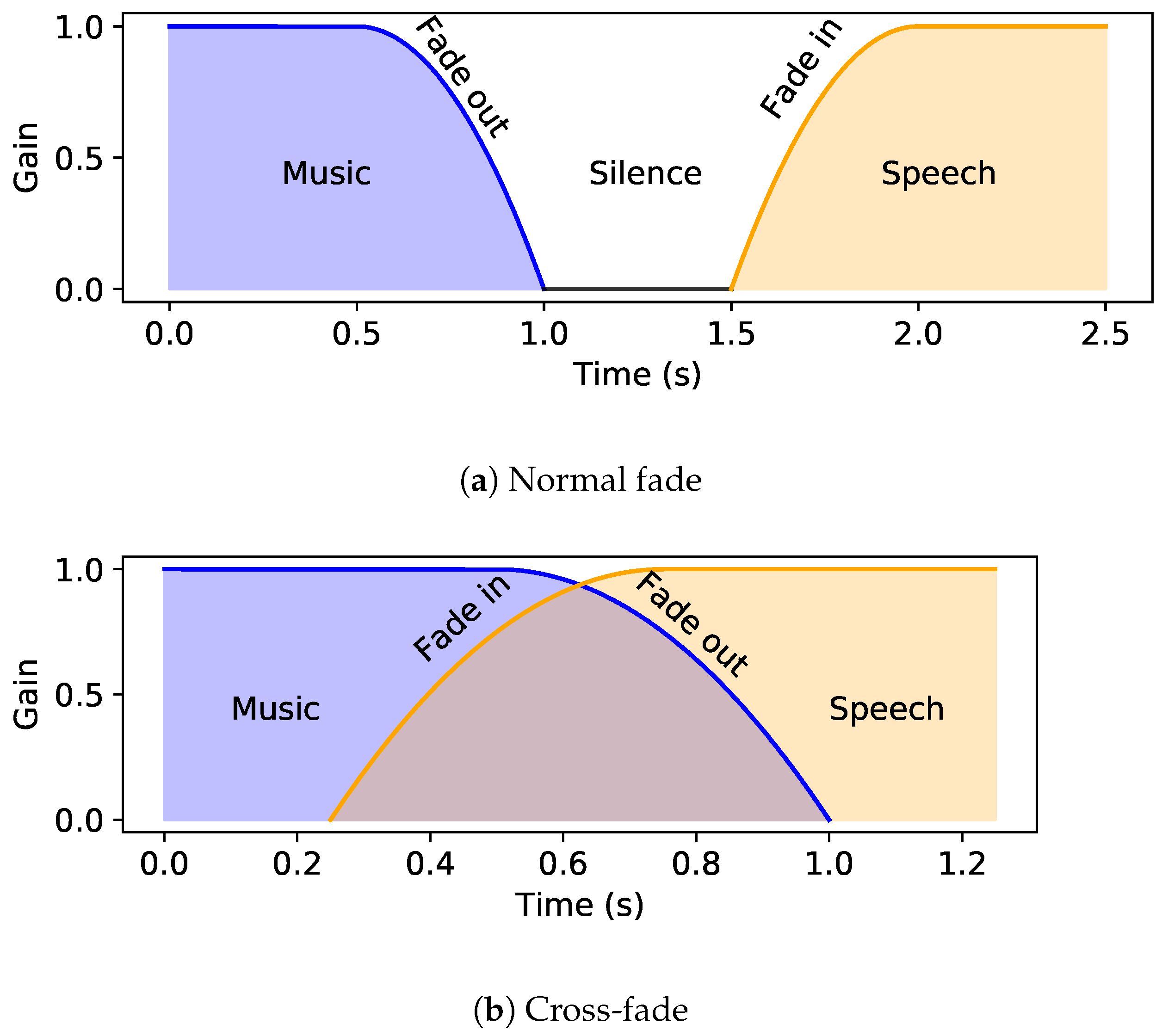
2.2. Audio Transitions

We observed two types of transition, which we termed as (1) normal fade transition and (2) cross-fade transition. In the former, an audio class fades out, followed a period of silence, and then a new acoustic class fades in. An example of this transition is when a Radio DJ introduces a song, followed by short gap, and then the song starts playing. In a cross-fade, a new acoustic class fades in while the old one is fading out. For instance, one song smoothly cross-fading into another song. Figure 1 illustrates the two types of audio transitions.
Each synthetic example can either have no transitions or at the most one transition. Hence, for a multi-class example, if there are no audio transitions, there are three possible occurrences—music, speech, or noise. If there is one transition, there are nine possible permutations between the classes. Note that we also included repetitions of the same audio class. For example, in an interview, two different voices occur with a pause. In radio broadcast, noise examples are less likely to occur when compared to speech and music. Therefore, the probability of music, speech, and noise was set to be 0.4, 0.4, and 0.2 respectively.
For multi-label examples, as shown in Figure 2, we performed audio ducking of background music, which is a common practice in broadcast audio. This process is explained in Section 2.6. If there are no audio transitions, there is only one possible combination—music+speech. If there is one audio transition, the possible permutations are given below.
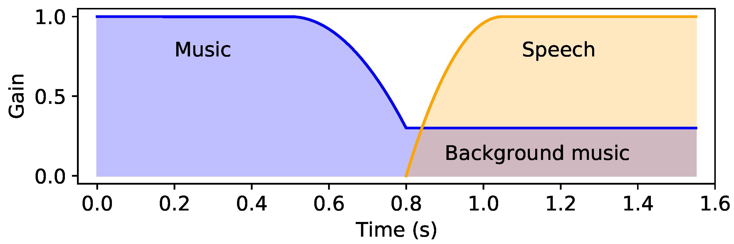
  • Music+speech to music: Initially, audio ducking is performed on the music and the volume is increased after the speech stops.
  • Music+speech to speech: The background music fades out at the transition point.
  • Music to music+speech: Initially, music is being played and ducking is performed when the speech starts.
  • Speech to music+speech: Music fades in at the transition point.

2.3. Time-Related Variables
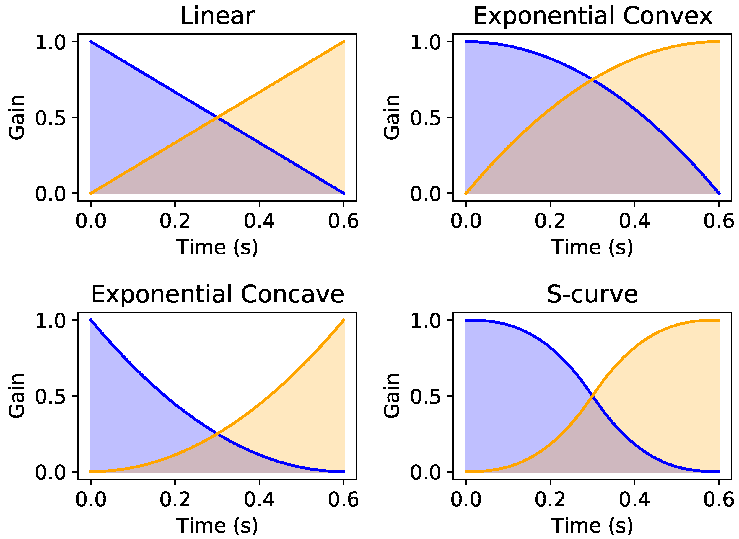
In real-world radio data, many parameters are generally defined by the mixing engineer. For example, duration of the fade curve and time-stamp of the audio transition. For our artificial data synthesis, we randomised these parameters to obtain a variety of synthetic examples. All random sampling was done using uniform distributions within specified ranges.
Within the duration of an 8 s example, the time-stamp of an audio transition is randomised within the range of 1.5 s to 6.5 s. Subsequently, a fade duration is randomised within a range that is feasible. For example, if the time-stamp of transition is at 5 s, the minimum fade out duration could be 0 s (which is no fade out) and a maximum of 3 s. This technique helps us render very quick as well as gradual audio transitions.

2.4. Fade Curves

When rendering an audio transition, mixing engineers can adopt a variety of fade curves. We considered the four most popular fade curves [12]—linear, exponential convex, exponential concave, and s-curve. Figure 3 shows the different types of fade curves.
For each audio transition, we randomly choose fade curves. For the exponential convex, exponential concave, and s-curve, we need to define an exponent value. The exponent value was randomly chosen between 1.5 to 3.0.

2.5. Sampling Audio Files

Audio files pertaining to each class are stored in separate folders. Initially, a template of the synthetic audio examples is designed by specifying the list of audio classes, transition points, etc. Then, a random file belonging to the required audio class is selected. Consequently, a random segment of the required duration is sampled within the audio file.

2.6. Audio Ducking

Audio ducking is the process of reducing one signal with respect to another. In this case, we reduce the volume of background music with respect to speech, in order to make speech more intelligible. Figure 2 shows an example of audio ducking in our system. This is a common practice in broadcast audio. Different radio stations have varying guidelines for mixing engineers to perform audio ducking. Torcoli et al. [13] conducted a comprehensive analysis on the loudness difference (LD) between speech and background music. Listeners from different backgrounds had varying preferences. On average, LDs preferred by experts were 4 Loudness Units (LU) less than those preferred by nonexperts. In addition, individuals belonging to older age groups preferred greater LDs to clearly understand speech.
The literature does not provide us with an ideal value for LD. It depends on the mixing engineer, target-audience, and nature of audio content. Many broadcasters recommend a minimum of 7 to 10 LU for speech over music. Others, for instance, the UK Digital Production Partnership, recommends a minimum LD of 4 LU [14].
Higher LDs cause the background music to become quieter. This leads to clearer speech, but the music becomes less impactful. Again, this depends on the nature of audio content. Depending on the programme, the LD could be as high as 23 LU [13]. Moreover, OpenBMAT, a music-detection, contains audio files as low as −51 Loudness Units relative to Full Scale (LUFS).
There are two ways to perform audio ducking—volume automation and side-chain compression. We have adopted the former technique because it is relatively easier to calculate LD values. Loudness of audio was calculated using the integrated loudness metric by ITU BS.1770-4 [15]. During data synthesis, we calculate the loudness of the speech segment. Subsequently, we adjust the gain of background music to the required LD. In this study, we evaluate how the network trains over different ranges of LDs. Section 5 presents the methodology for these experiments.
Figure 4 depicts an overview of the data synthesis procedure. Note that in cases where audio ducking is performed, the network needs to predict the presence of both music and speech. In addition, when an audio class is fading in or out, the entire fade curve is labelled as 1. We do not consider power of the audio with respect to the mixture gain.
Unless mentioned otherwise, the probabilities for all events were equally weighted. For example, the chance of occurrences for multi-label and multi-class examples are 50% each. Four fade curves were considered in the paper and thus, each fade curve has a probability of 25%. Similarly, the probabilities for other events were calculated based on the total possible number of occurrences.

3. Methods

3.1. Preprocessing and Feature Extraction

Audio was resampled to 22.05 kHz mono files. As we are performing segmentation-by-classification, silences in these audio files would be unrepresentative of the audio class, for instance, pauses in speech. Therefore, we removed/shortened silences in the audio files by using Sound eXchange (SoX) (http://sox.sourceforge.net/, accessed on 26 February 2021).
For our data synthesis to work smoothly, it is convenient to have audio files with a minimum duration of 8 s. Music files in the IRMAS dataset are only 3 s long. In addition, some speech examples in LibriSpeech and noise examples in MUSAN are shorter than 8 s. Therefore, we looped these audio files multiple times to reach the required duration.
Studies have generally used Mel spectrograms or Mel-frequency cepstral coefficients (MFCCs) as audio features [2,8]. We extracted 80 log-scale-Mel bands in the range of 64 Hz to 8 kHz. The hop size and fast Fourier transform (FFT) size were set to 220 (10 ms) to 1024 (46 ms) respectively. Features were extracted using Librosa [16].
Audio segments were peak-normalised before passing them through the pipeline for data synthesis. Finally, the whole audio file was peak-normalised after synthesis.

3.2. Datasets

3.2.1. Repository for Data Synthesis

To generate audio that resembles a radio broadcast, we aggregated a data repository that contains audio files labelled as either music or speech. Please note that these files are not mixed and contain only one acoustic class. Among the datasets popularly used for music-speech detection, we included the MUSAN corpus [17], GTZAN music and speech detection dataset [18], and the Scheirer and Slaney dataset [19]. After analysing errors in early informal experiments, without having access to the test set, we observed that speech was confused with wind instruments like flute. Hence, we included the Instrument Recognition in Musical Audio Signals (IRMAS) dataset [20] that includes many examples of wind instruments and GTZAN genre recognition [21] for additional music examples.
It was also challenging for the network to differentiate between singing voice and spoken voice. Therefore, we included a part of the LibriSpeech corpus [22], which serves as a good collection of speech examples. In addition, vocal sections without musical accompaniment is harder to identify. Thus, we included the Singing Voice Audio Dataset [23] which contains unaccompanied vocals.
To enable the network to identify task-irrelevant data, we added noise examples from MUSAN corpus. This included environmental sounds, unintelligible speech, and sound effects, to name but a few. The total number of unique audio files for music, speech, and noise was 6876, 6885, and 665 respectively.

3.2.2. Real-World Radio Data

The MuSpeak dataset contains seven audio files and has a total length of approximately 5 h. Two, three, and two audio files were used for training, validation, and testing respectively. We did not split the audio files to prevent the risk of having similar content across different dataset splits.
We also collected 18 h of radio broadcast from BBC Radio Devon. We annotated the audio files for the presence of music and speech. For convenience, we split the audio into files of 1 h. We created an approximate split of 50-30-20% for training, validation, and testing respectively. As we are working with radio data, there are occasional repetitions of audio segments such as jingles. Extra care was taken to minimise repetition across the different dataset splits.
Three hours of our annotations on the BBC data were verified by an external audio mixing engineer. He was paid for his time and was not involved in the research. Additionally, a random section of 15 min was blind-annotated by him independently. We found an agreement of 99.49% with our annotations by using 10ms segment verifications. This was done to ensure that audio events were similarly perceived by different people.
In this paper, we investigate the use of artificially synthesised data as training sets. In Section 7, we compare the model’s performance on different training sets—for instance, synthetic data versus real-world data. In all cases, we used only real-world data for validation and testing.
We also tested our models on the MIREX music and speech detection competition dataset. This helps us understand how our models generalise to data from other distributions. This dataset contains 27 h of audio from various TV programmes.

3.3. Postprocessing and Evaluation

The neural network was designed to make predictions over 8 s audio. During testing, for files that were longer than 8 s, we traversed the audio with a window size of 8 s and a hop size of 6 s. Within each 8 s-window, we discarded the predictions for the first and last second of audio, because the border-predictions might unreliable. This method was adopted from the paper by Gimeno et al. [8]. Suppose the audio was less than 8 s long; the signal was right padded with zeros to obtain the required duration.
The predictions made by machine learning models are generally passed through a postprocessing or smoothing stage. This is done to eliminate spurious audio events. The literature has two popular techniques—median filtering [6,8] or setting thresholds for minimum durations of audio events [7]. We adopted the latter approach. The minimum durations for speech and music were 0.8 s and 3.4 s respectively. The maximum silences between speech and music events were 0.8 s. These values were adapted from the study by Lemaire et al. [7] and were manually adjusted to suit our in-house dataset.
We evaluated our segmentation models using the sed_eval toolbox [24], which has been popularly adopted by the literature [7,25,26]. Segment-level evaluation was performed with a segment size of 10 ms. All experimental results in this paper were presented after smoothing the predictions made by the machine learning models.

4. Experiment I: Comparison of Neural Network Architectures

4.1. Experimental Set-Up

Recently, many studies have adopted deep learning for audio segmentation and classification. State-of-the-art architectures include Convolutional Neural Network (CNN) [27,28,29], Bidirectional Long Short-Term Memory (B-LSTM) [8], Bidirectional Gated Recurrent Unit (B-GRU) [30], Convolutional Recurrent Neural Network (CRNN) [25,31,32], and Temporal Convolutional Neural Network (TCN) [7]. CRNN and TCN generally outperform the other architectures because they take advantage of both convolutional and recurrent layers [7]. In this paper, we compare state-of-the-art architectures to choose the best one for our task.
The training set used for hyperparameter tuning was a combination of real-world data and artificially synthesised data, which was approximately 10 h and 23 h respectively. The input layer for each neural network was 802 × 80 × 1 , corresponding to 802 times steps and 80 Mel bins. The output of each network had 802 × 2 neurons with sigmoid activations. Two neurons performed a binary classification for speech and music separately at each time step. Please note that the model performed multi-output detection, where the occurrences of music and speech are mutually exclusive. All neural networks were trained using the Adam optimiser [33] with a learning rate of 0.001. The loss function was binary cross-entropy.
Techniques like batch normalization (BN) [34] and layer normalization (LN) [35] are adopted to speed up the training process in neural networks. These methods also provide the benefit producing a regularization effect. Ba et al. [35] showed that LN was more effective than BN for recurrent architectures like LSTM and GRU. However, BN is more effective for CNNs.

4.1.1. CNN

For the CNN, we passed the input through a set of 2D convolution layers. After each convolution layer, we performed batch normalization, ReLU activation, and Max pooling. Max pooling was performed only on the frequency axis in order to maintain the time resolution of the network. After the convolution blocks, we had a set of fully connected (FC) layers. Each FC layer was followed by dropout.

4.1.2. B-LSTM and B-GRU

We passed the input through a series of B-LSTM or B-GRU layers. All layers used tanh activation functions. Initial tests showed that LN was considerably more effective than BN for B-GRU and B-LSTM networks. In addition, we observed that a combination of dropout and LN adversely affected the performance of the network. Hence, each recurrent layer was followed by only LN and no dropout.

4.1.3. ncTCN

TCN is a family of architectures that perform 1D convolutions on sequential data. They are known to perform better than B-LSTM and B-GRU architectures on a vast range of tasks [36]. Lemaire et al. [7] proposed the noncausal TCN (ncTCN) for audio segmentation, which passes the sequence forward and backward, similar to B-LSTM. The study also showed that ncTCN was more effective than TCN for segmentation.
For our study, ncTCN was implemented by using this GitHub repository (https://github.com/philipperemy/keras-tcn, accessed on 26 February 2021). The input was passed through a series of ncTCN layers. We did not observe difference in performance between LN and BN. Hence, LN was applied after each layer to maintain uniformity with B-LSTM and B-GRU.

4.1.4. CRNN

CRNN, as the name suggests, comprises a series of convolution layers followed by recurrent layers. Similar to TCN, we did not observe a noticeable difference between LN and BN and thus, used LN for the network. The input was passed through a set of 2D convolutions. Each convolution was followed by ReLU activation, Max pooling, and LN. After the convolution blocks, we had a series of B-GRU layers, each of them followed by LN.

4.1.5. Hyperparameter Tuning

For each network, hyperparameter tuning needs to be performed separately. To present an unbiased comparison, we adopted an automatic hyperparameter method called Hyperband [37]. The list of hyperparameters explored for each architecture can be found in Table 1. For tuning, we set the maximum number of epochs to 10 and the Hyperband factor to 3.
During hyperparameter tuning, we set the batch size to 32 to fit large models in the RAM. For each of the architectures, after an optimal network was chosen by Hyperband, we trained the networks for an extended number of epochs. Early-stopping [38] with a patience of 20 epochs was implemented during training and the model obtaining the lowest validation error was selected. In addition, we decayed the learning rate by a factor of 0.84 after 10,000 weight updates.

4.2. Results

The parameters chosen by Hyperband can be found in Table 2.
Table 3 presents the results of different architectures on the validation and test set. For the overall F-measure, the CRNN network evidently outperformed other models. It also obtained the highest speech F-measure in both datasets. CNN obtained a high music F-measure on the validation set and interestingly the highest F-measure on the test set. However, its speech F-measure was poorer. Studies have explained that music tends to have more stationary parts than speech [39]. Moreover, Jang et al. [40] adopted a CNN for music detection in radio broadcast. Our results show that CNNs are excellent for music detection but not for speech detection.
There was not much difference between the B-LSTM and ncTCN architectures. Bai et al. [36] had stated that TCNs perform better than recurrent architectures because they exhibit longer effective memory. However, the examples in our training set have a fixed duration of 8 s. It is probable that the longer memory of TCN was not advantageous for our task.
Unlike TCN, the CRNN model also performs convolutions on the frequency axis, which contributes to its better performance. During initial experiments, we also observed 2D convolutions were more effective than 1D convolutions.
The CRNN model that was selected by Hyperband had 2.4 million parameters. For further experiments in this paper, the chosen model was unnecessarily large and was beyond our computational budget. We reduced the number of filters from 128 to 64 in the first two convolution layers. This reduced number of parameters to approximately 700 thousand and had a negligible impact on performance. Moreover, we increased the batch size from 32 to 128 to speed up training. In addition, we updated the learning rate schedule to decay by a factor of 0.84 after 2500 weight updates. The smaller model is labelled as “CRNN-small” and the results are presented in Table 3. Furthermore, the smaller model obtained the highest overall F-measure on the test set. However, our decision was informed only by the validation set.

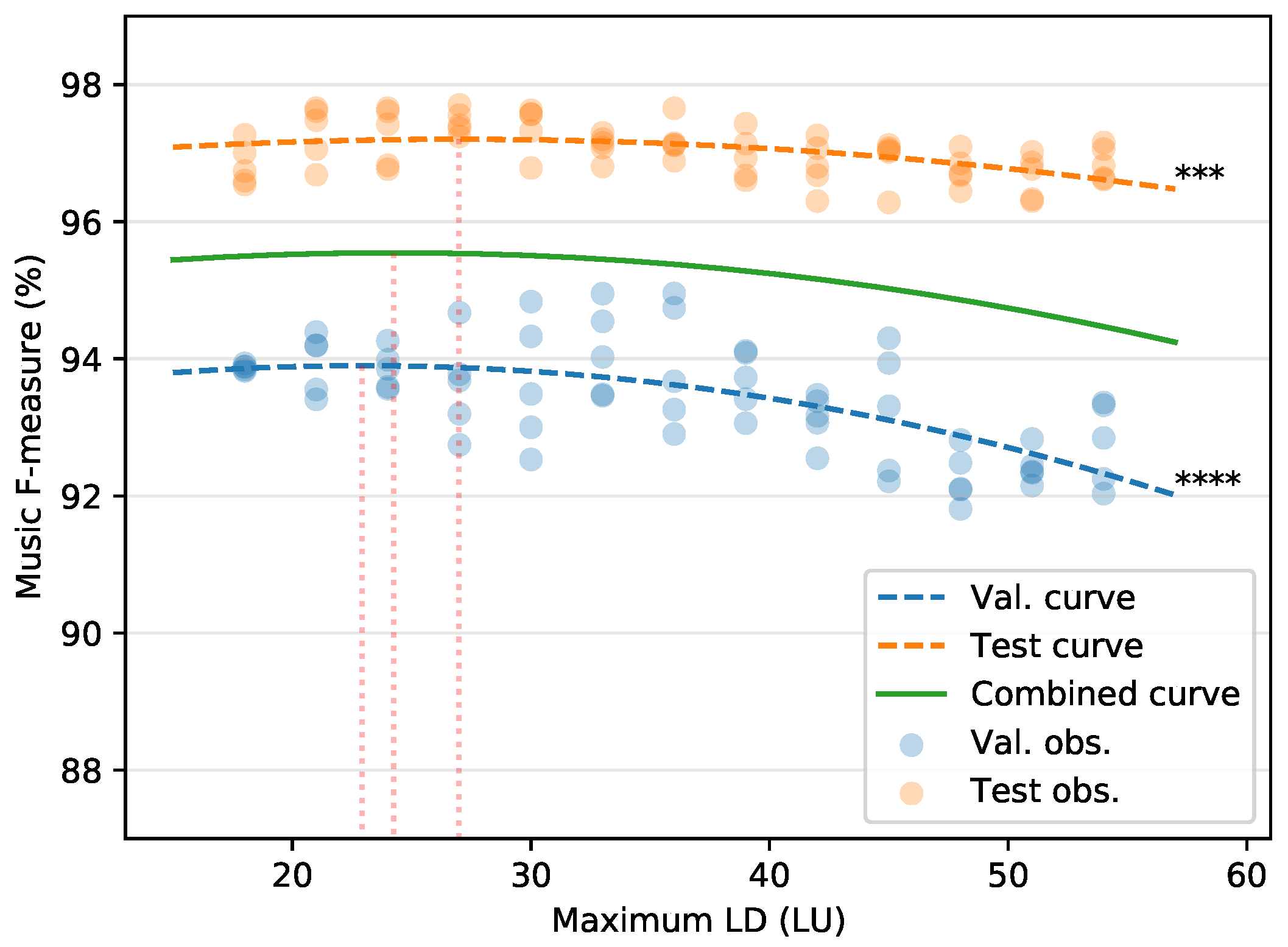
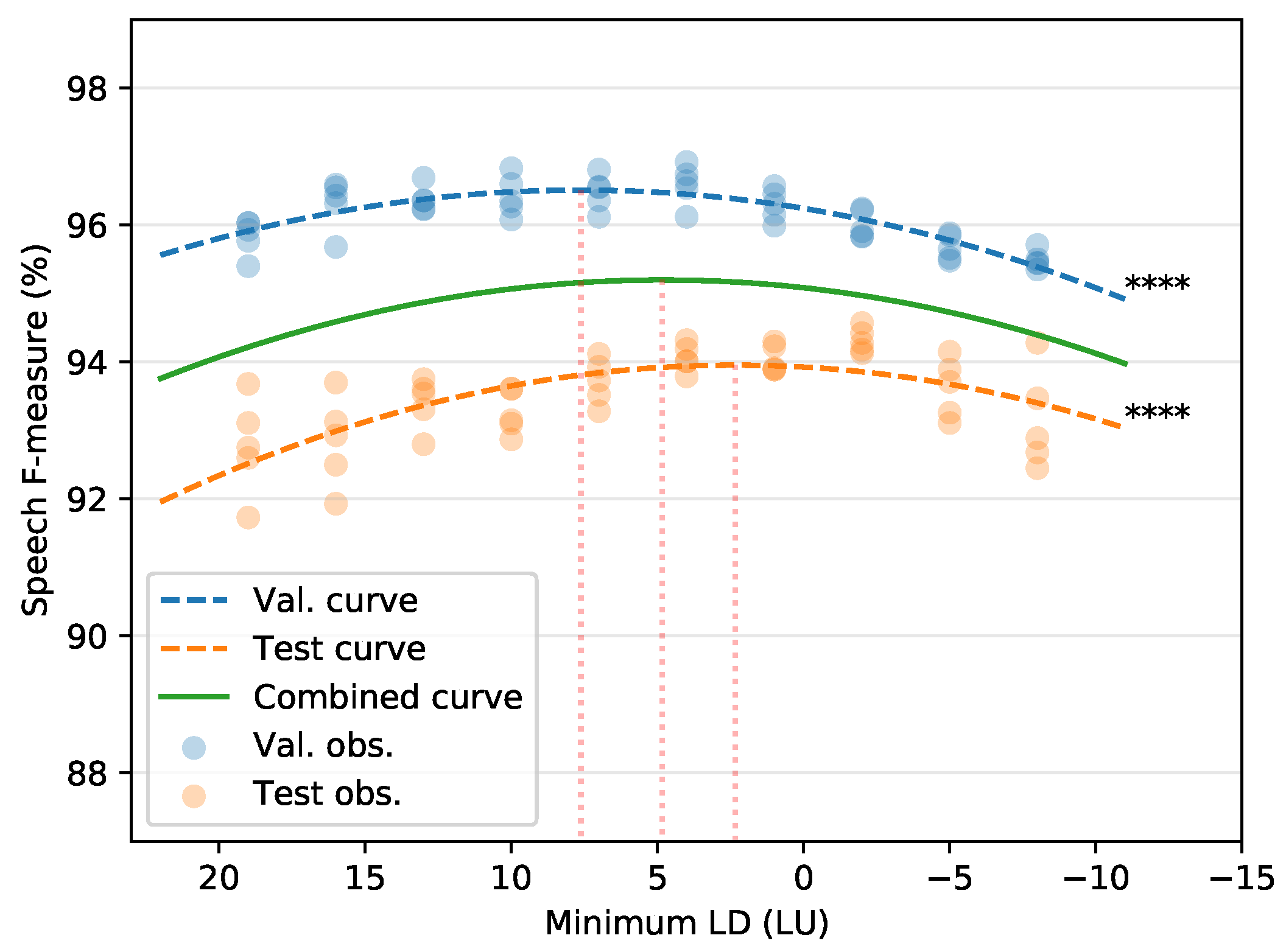
5. Experiment II: Loudness Difference Selection

5.1. Experimental Set-Up

In this experiment, we used only synthetic data to train the neural network. For each audio example with speech over background music, we need to select an LD between the audio classes. This LD cannot be constant because the neural network will become biased towards learning a specific LD. Therefore, we chose random LD values from a uniform distribution. However, the literature does not provide us with a clear-cut range of LDs. For our data synthesis procedure, we need to select an optimal maximum and minimum value of LD.
First, we set the minimum value at 7 LU. The maximum value was varied from 18 to 54 LU with steps of 3 LU. We synthesised 5120 examples and trained the network over these examples for each configuration. The choice of maximum LD is expected to only influence the performance on music. The greater the LD, the lower the volume of background music and vice versa. If the background music is sufficiently loud, we can precisely detect the presence of music. However, if the background music becomes too low, it becomes harder for the listener to precisely detect the presence of music. Hence, we analysed the precision, recall, and F-measure of music. We repeated the experiment five times using different random seeds. Regression analysis was performed on the observations using SPSS [41]. Analysis of variance (ANOVA) was conducted to evaluate the level of significance.
Similarly, we set the maximum value at 21 LU and the minimum value was varied from 19 to −8 LU with a step of −3 LU. The smaller the LD, the louder the background music is. Negative LDs stand for cases when the background music is louder than the speech. Therefore, if the LD is too low or negative, we expect the precision of speech to be hindered. This often occurs in advertisements and radio jingles, which have smaller LDs. Again, for each configuration, we synthesised 5120 examples and trained the network over these examples. The minimum LD is expected to only influence the intelligibility of speech. Hence, we analysed the precision, recall, and F-measure of speech. We repeated the experiment five times. Regression analysis and ANOVA were performed on the observations.

5.2. Results

5.2.1. F-measure

F-measure is a metric that combines precision and recall by calculating their harmonic mean [42]. Figure 5 presents a quadratic regression of how the F-measure of music changes with maximum LD. The maxima for validation, test, and combined curves lie at 23, 27, and 24 LU respectively. The validation and test curves were significant ( p < 0.001 ). However, the combined curve that jointly plots validation and test observations was not significant ( p > 0.05 ). Therefore, our results suggest that the optimal value of maximum LD lies somewhere between 23 and 27 LU.
Torcoli et al. [13] suggested that depending on the nature of broadcast content, the LD can be as high as 23 LU, which has a reasonable overlap with our findings. However, we did not find a single optimal value for maximum LD based on F-measure but a range of values from 23 to 27 LU.
Figure 6 shows a regression analysis of how the F-measure of speech varies with minimum LD. The maxima for validation, test, and combined curves lie at 8, 2, and 5 LU respectively. The validation and test curves were significant ( p < 0.0001 ). However, the combined curve that jointly plots validation and test observations was not significant ( p > 0.05 ). Therefore, our results suggest that the optimal value of minimum LD lies somewhere between 2 and 8 LU.
As explained in Section 2.6, many broadcasters recommend a minimum of 7 to 10 LU for speech over music and some recommend a minimum LD of 4 LU [13,14]. Note that these are only recommendations to make speech intelligible. However, there are cases where mixing engineers choose LDs close to zero or even negative LDs [13]. Therefore, in order to maximise F-measure, our results suggest that the minimum LD should lie between 2 and 8 LU.
As the F-measures of combined curves were statistically insignificant, it may benefit from further analysis. Are we overfitting the validation set? Or is there an optimal LD for different datasets? To address the questions, we analysed precision and recall in the following subsection.

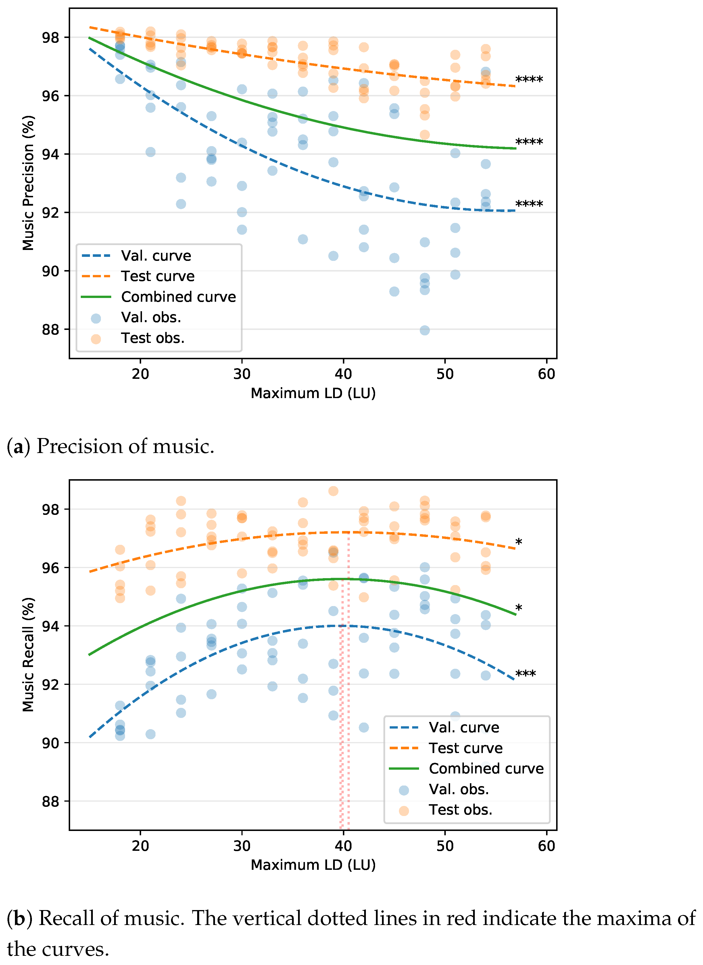
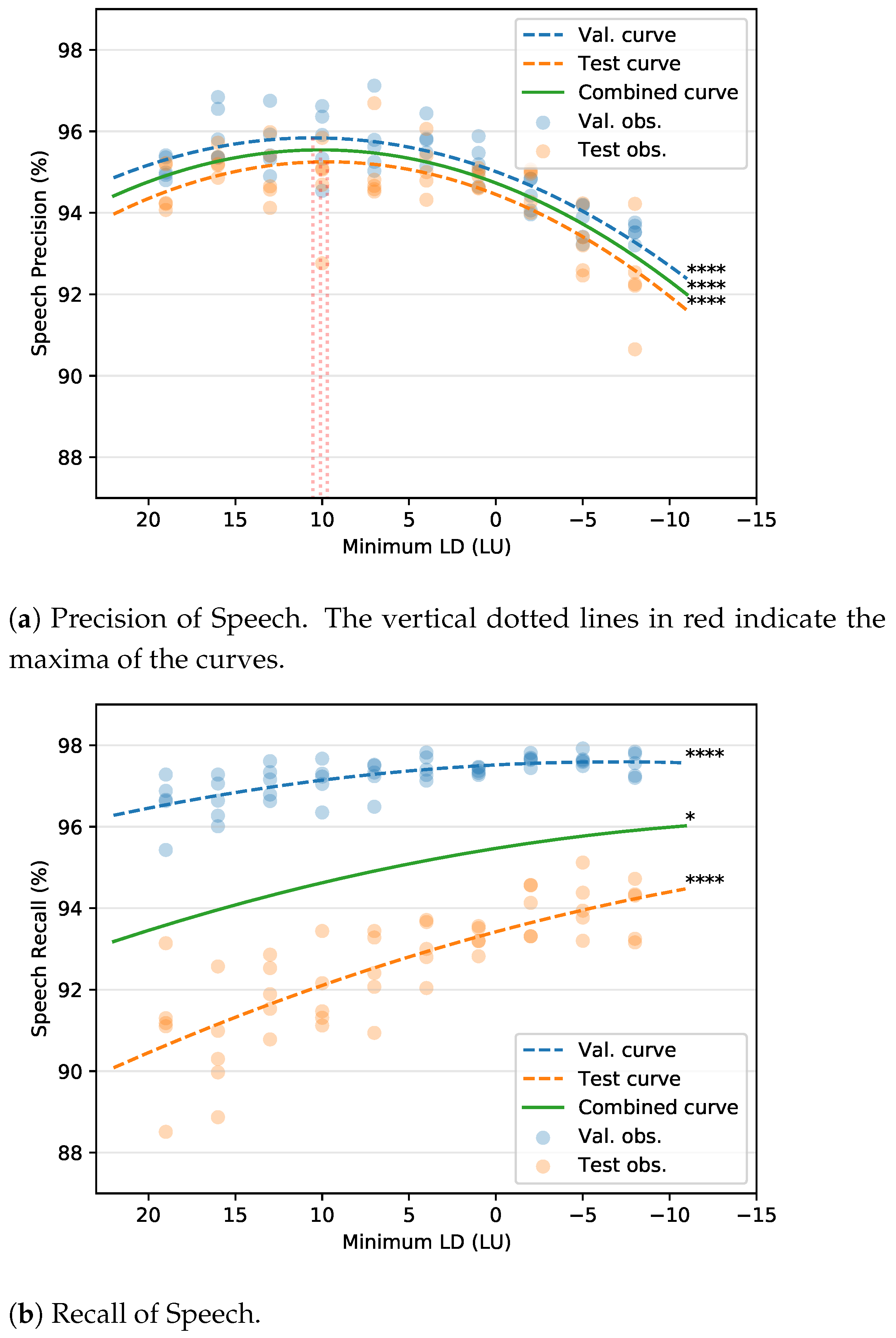
5.2.2. Precision and Recall

Figure 7a presents a regression analysis of how precision of music varies with maximum LD. A quadratic curve was fitted to the observations. All curves evidently demonstrate than precision decreases as the maximum LD increases ( p < 0.0001 ). Therefore, if the neural network was trained on examples that have very low volumes of background music, the precision is hindered.
On the other hand, Figure 7b shows the relationship between recall of music and maximum LD. Initially, recall increases as the LD increases. However, the maxima for the validation, test, and combined curves lie approximately at 40 LU. This shows that the recall does not increase beyond an LD of 40 LU. In other words, the background music becomes too low to be perceived. Hence, we recommend that the maximum LD should never be greater than 40 LU, even if the researcher desires a high recall.
Figure 8a shows a regression analysis of speech precision with regards to minimum LD. Initially, as the minimum LD decreases, there is an increase in precision. The maxima for all the curves lie at approximately 10 LU. Below 10 LU, there is a decrease in precision. This is an interesting observation because the same LD is preferred by human listeners [13]. Torcoli et al. [13] conducted a study on the LDs preferred by human listeners. Based on the test results, they recommended a minimum of 10 LU between speech and background music. Contrarily, many broadcasters use LDs less than 10 LU, which makes speech intelligible [13]. It is noteworthy that machine learning models in this study also preferred a minimum LD of 10 LU to maximise the precision of speech.
Figure 8b shows that recall continuously improves with a decrease in minimum LD. This is because the machine learning model learns more examples where speech and background music have a small LD. This also shows that the real-world radio examples collected from BBC Radio Devon contain cases where speech and background music have small LDs. However, as shown in Figure 8a, the precision of speech is affected in these cases.
The results in this subsection and Section 5.2.1 clearly demonstrate that there is a trade-off between precision and recall when selecting a maximum and minimum LD. A researcher may adjust these settings according to their objectives. Moreover, F-measure assigns an equal weightage to precision and recall, which might not be desirable. For further experiments in our study, we did not make any decisions based on the regression analysis because it includes the test set. Instead, we chose values that obtained the highest mean for F-measure on our validation set. The minimum and maximum LD were set to 4 and 33 LU respectively.

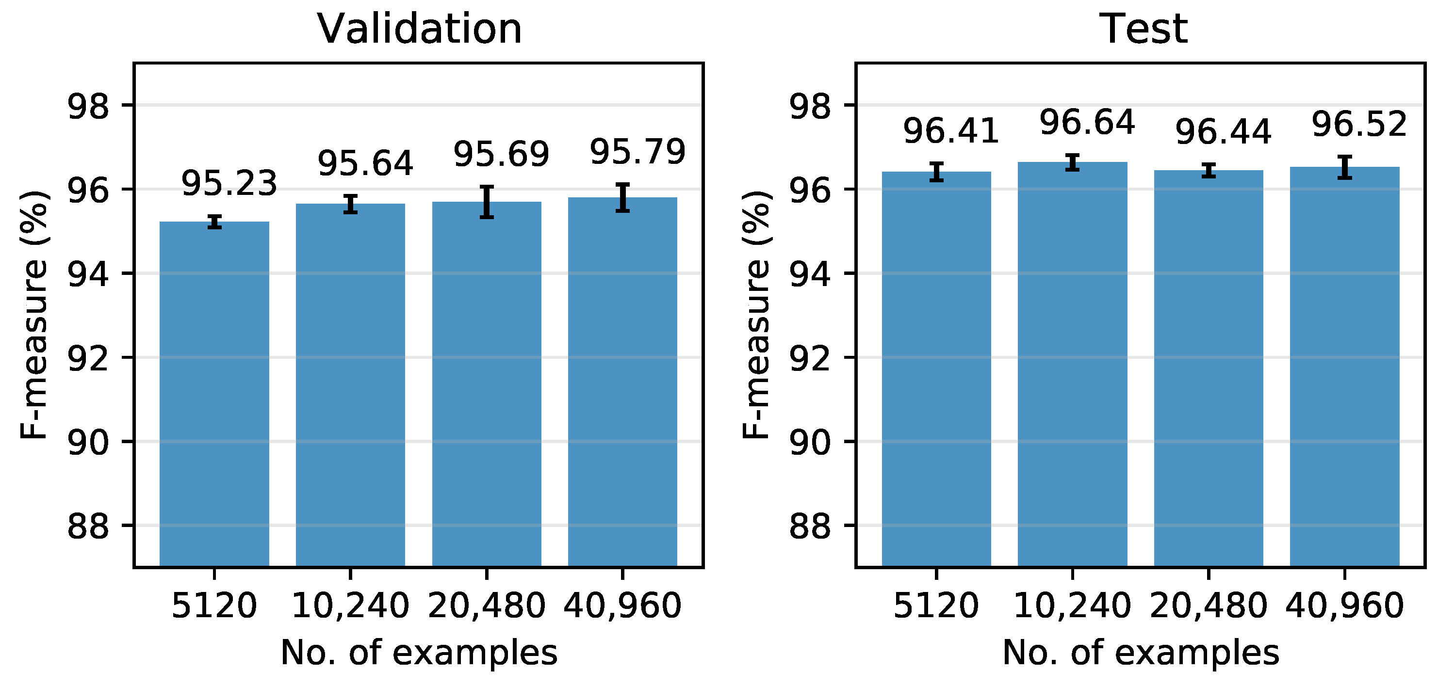
6. Experiment III: Size of the Dataset

6.1. Experimental Set-Up

As we are artificially synthesising training data, we have the flexibility to create large training sets. To develop an understanding of how the network’s performance improves with the size of the training set, we evaluated the performance over 5120, 10,240, 20,480, and 40,960 examples. To evaluate the significance level, a two-way ANOVA was performed with dataset size and dataset type (validation and test) as factors. A posthoc Tukey test was performed to make pairwise comparisons.
The number of unique speech and music files in the data repository are only 6885 and 6876 respectively. In order to manage redundant examples, we adopted a new training strategy. For every training cycle, we randomly select 40 mini-batches and calculate the error on the validation set. This way, we prevent the risk of overfitting within epochs. This training strategy was adapted from the study by Schlüter et al. [43]. However, we used the Adam optimiser with the same learning rate schedule explained in Section 4.2.

6.2. Results

Figure 9 plots the overall F-measure against different training set sizes. We did not observe any patterns in precision and recall because in this section, the minimum and maximum LD values were constant at 4 and 33 LU. As we increased the size of the training set, we observed a slight increase in F-measure on the validation set. However, on the test set, an increase was found from 5120 to 10,240 examples but not on subsequent intervals. ANOVA showed that the dataset size had a significant effect on the F-measure ( p < 0.05 ). Posthoc tests showed that there were significant differences for two pairs—(5120 & 10,240) and (5120 & 40,960). All the other pairs were statistically insignificant. Therefore, we can conclude that the performance does not significantly improve beyond 10,240 training examples. This might be due to our data repository comprising approximately 6800 unique examples for each audio class.
For the next experiment in our paper, we used 40,960 training examples instead of 10,240 examples. This is because 40,960 examples obtained the highest F-measure on our validation set and we did not make any decisions based on the test set.

7. Experiment IV: Comparison of Real-World and Artificial Data

7.1. Experimental Set-Up

To evaluate the effectiveness of our data synthesis algorithm, it is important for us to compare the performance with real-world data. Therefore, we trained the model on four different training sets as shown below. Each of them comprised of 40,960 8 s-long audio examples.
  • SSE: Sound segment examples (SSE) consisted of audio directly sampled from the data repository. This does not contain mixed audio.
  • SSE+RRE: This is the combination of SSE and Real-world radio examples (RRE). This is the type of training set used by most audio segmentation studies.
  • ARE+RRE: In this set, we used a combination of Artificial Radio Examples (ARE), which are synthesised using our data synthesis procedure and RRE.
  • ARE: Here, we used only ARE for training the model.
During training, to manage redundant examples, we adopted the same training strategy as explained in Section 6.1. All the four models were tested on our in-house dataset and the MIREX competition dataset. Similar to earlier experiments, we trained models for five iterations of data synthesis using different random seeds. However, we created an ensemble of the five models. A simple average [44,45] over the sigmoid outputs of the five networks was calculated to obtain the final prediction. By creating an ensemble, we would obtain a single number evaluation on our test set instead of means and standard deviations. Therefore, we can compare our models with state-of-the-art algorithms submitted to the MIREX competition, which adopt the same testing paradigm. Moreover, a group of networks reduces generalisation error by combining predictions [44,45].

7.2. Results

The models were trained using four different training sets—SSE, SSE+RRE, ARE, and ARE+RRE. Table 4 shows the evaluation on our in-house dataset. SSE and ARE comprise examples from the same data repository. However, ARE increases the overall F-measure by 4.5%. This demonstrates the effectiveness of the data synthesis algorithm.
SSE+RRE is the type of training set generally used by audio segmentation studies [7]. Interestingly, the overall F-measure of ARE also surpasses SSE+RRE. Considering the fact that RRE belongs to the same data distribution as the test set, this is a significant development.
ARE+RRE evidently outperforms the other models. It harnesses the advantage of both synthetic radio examples and real-world data.
The upper half of Table 5 presents the results of our models on the MIREX competition dataset. We observe similar trends as the results in Table 4—ARE outperforms SSE and SSE+RRE. Interestingly, ARE has higher F-measure for music than ARE+RRE but obtains lower speech F-measure. It is important to note that in this case, the training and test datasets were annotated by different research groups. Therefore, there would be disagreements in annotations for low volumes of background music. This trend was also observed in the OpenBMAT dataset [10], which had low agreement percentages across annotators for background music in very low volumes. The advantage of artificially synthesising data is that it is independent of this human error in labelling. Contrarily, in speech annotations, there are less scope disagreements. Therefore, ARE+RRE has higher Speech F-measure than ARE.
The lower half in Table 5 shows the previously published results obtained from the MIREX website. The music F-measure of all our models surpassed the performance of earlier submissions. This can be attributed to the variety of datasets in our data repository. The submissions by Marolt et al. [47] surpassed three of our models in speech F-measure. However, ARE+RRE obtained a higher speech F-measure.
The ARE model in Table 5 obtained slightly poorer results than the one presented in our previous study [11]. This is because we used a different neural network. In the current paper, hyperparameter tuning was performed on ARE+RRE by using Hyperband. However, in the previous study [11], we manually optimised the network for only ARE. Additionally, we had included dropout for regularisation and used BN instead of LN.

8. Conclusions

In this study, we evaluated the challenges involved in synthesising data that resembles radio broadcast. We surveyed the literature to understand the various mixing principles adopted by broadcasting stations. We incorporated fade curves to smoothly render transitions and audio ducking to facilitate the intelligibility of speech.
We evaluated state-of-the-art neural network architectures for the task of audio segmentation and observed that CRNN outperformed other models. This paper also investigated the impact of LD between speech and background music while training neural networks. There was a trade-off between precision and recall when selecting maximum and minimum LDs. Moreover, if the LD was less than 10 LU, the precision of the network gets affected. This choice of minimum LD for the machine learning model was similar to that of human listeners in the literature [13]. This paper also recommended that the LD between speech and background music should not be greater than 40 LU because the music becomes too quiet to be detected. This emphasises that the task of background music-detection needs to be defined in greater detail by using threshold-related variables.
The results demonstrated that our data synthesis procedure is a highly effective technique to create large-scale training sets. We compared the effectiveness of real-world and synthetic training sets. Interestingly, artificial data surpasses the performance of real-world data in some scenarios. It generalises better to other data distributions because it does not depend on human annotations.
As this paper has significantly reduced the time and resources required to label datasets, it opens up many possibilities for future work. Audio features like Mel spectrograms and MFCCs discard the phase of the audio and only consider its magnitude. This might hinder the algorithm’s ability to capture audio transitions. End-to-end deep learning, as suggested by some researchers [7,48], seems like a promising approach to audio segmentation. The results in Section 6.2 showed that the performance did not significantly improve beyond 10,240 examples. This suggests that other methods such as Generative Adversarial Networks (GANs) [49,50] might improve the quality of synthetic training sets.

Author Contributions

Conceptualization, S.V., D.M. and E.R.M.; investigation, S.V.; software, S.V.; visualization, S.V. and D.M.; writing—original draft, S.V.; writing—review and editing, D.M. and S.V.; supervision, D.M. and E.R.M.; project administration, E.R.M.; funding acquisition, E.R.M. All authors have read and agreed to the published version of the manuscript.

Funding

This study was supported by Engineering and Physical Sciences Research Council (EPSRC) grant EP/S026991/1.

Data Availability Statement

The repository for data synthesis in this paper comprised only openly available datasets. We do not have the permission to share these datasets, but they can be accessed online or by contacting the respective authors. The code to synthesise radio examples is openly available in this GitHub repository (https://github.com/satvik-venkatesh/train-synth-audio-seg/, accessed on 26 February 2021). The data provided by BBC Radio Devon is copyrighted material and cannot be shared. However, MuSpeak [9] is an openly available annotated dataset, which can be utilised by researchers for validation and testing.

Acknowledgments

The authors thank BBC Radio Devon for providing us with 18 h of broadcast audio. We also thank Clive Mead, the external audio mixing engineer who verified our annotations. The deep learning research in this paper was conducted using Google Colab. The authors are grateful to this cloud computing service.

Conflicts of Interest

The authors declare no conflict of interest.

Abbreviations

The following abbreviations are used in this manuscript:
Algo.Algorithm
ANOVAAnalysis of variance
AREArtificial Radio Examples
B-GRUBidirectional Gated Recurrent Unit
B-LSTMBidirectional Long Short-Term Memory
BNBatch Normalization
CNNConvolutional Neural Network
CRNNConvolutional Recurrent Neural Network
FFTFast Fourier Transform
LDLoudness Difference
LNLayer Normalization
LULoudness Units
MIREXMusic Information Retrieval Evaluation eXchange
MFCCMel-Frequency Cepstral Coefficients
ncTCNNoncausal Temporal Convolutional Neural Network
Obs.Observations
OpenBMATOpen Broadcast Media Audio from TV
RREReal-world Radio Examples
SSESound Segment Examples
TCNTemporal Convolutional Neural Network
Val.Validation

References

  1. Theodorou, T.; Mporas, I.; Fakotakis, N. An overview of automatic audio segmentation. Int. J. Inf. Technol. Comput. Sci. 2014, 6, 1. [Google Scholar] [CrossRef] [Green Version]
  2. Butko, T.; Nadeu, C. Audio segmentation of broadcast news in the Albayzin-2010 evaluation: Overview, results, and discussion. EURASIP J. Audio Speech Music Process. 2011, 2011, 1. [Google Scholar] [CrossRef] [Green Version]
  3. Xue, H.; Li, H.; Gao, C.; Shi, Z. Computationally efficient audio segmentation through a multi-stage BIC approach. In Proceedings of the 2010 3rd IEEE International Congress on Image and Signal Processing, Yantai, China, 16–18 October 2010; Volume 8, pp. 3774–3777. [Google Scholar]
  4. Huang, R.; Hansen, J.H. Advances in unsupervised audio classification and segmentation for the broadcast news and NGSW corpora. IEEE Trans. Audio Speech Lang. Process. 2006, 14, 907–919. [Google Scholar] [CrossRef]
  5. Wang, D.; Vogt, R.; Mason, M.; Sridharan, S. Automatic audio segmentation using the generalized likelihood ratio. In Proceedings of the 2008 2nd International Conference on Signal Processing and Communication Systems, Gold Coast, QLD, Australia, 15–17 December 2008; pp. 1–5. [Google Scholar]
  6. Schlüter, J.; Sonnleitner, R. Unsupervised feature learning for speech and music detection in radio broadcasts. In Proceedings of the 15th International Conference on Digital Audio Effects (DAFx), York, UK, 17–21 September 2012. [Google Scholar]
  7. Lemaire, Q.; Holzapfel, A. Temporal Convolutional Networks for Speech and Music Detection in Radio Broadcast. In Proceedings of the 20th International Society for Music Information Retrieval Conference (ISMIR), Delft, The Netherlands, 4–8 November 2019. [Google Scholar]
  8. Gimeno, P.; Viñals, I.; Ortega, A.; Miguel, A.; Lleida, E. Multiclass audio segmentation based on recurrent neural networks for broadcast domain data. EURASIP J. Audio Speech Music Process. 2020, 2020, 5. [Google Scholar] [CrossRef] [Green Version]
  9. MuSpeak Team. MIREX MuSpeak Sample Dataset. 2015. Available online: http://mirg.city.ac.uk/datasets/muspeak/ (accessed on 26 February 2021).
  10. Meléndez-Catalán, B.; Molina, E.; Gómez, E. Open broadcast media audio from TV: A dataset of TV broadcast audio with relative music loudness annotations. Trans. Int. Soc. Music. Inf. Retr. 2019, 2, 43–51. [Google Scholar] [CrossRef] [Green Version]
  11. Venkatesh, S.; Moffat, D.; Kirke, A.; Shakeri, G.; Brewster, S.; Fachner, J.; Odell-Miller, H.; Street, A.; Farina, N.; Banerjee, S.; et al. Artificially Synthesising Data for Audio Classification and Segmentation to Improve Speech and Music Detection in Radio Broadcast. arXiv 2021, arXiv:2102.09959. [Google Scholar]
  12. Tarr, E. Hack Audio: An Introduction to Computer Programming and Digital Signal Processing in MATLAB; Routledge: Abingdon-on-Thames, UK, 2018. [Google Scholar]
  13. Torcoli, M.; Freke-Morin, A.; Paulus, J.; Simon, C.; Shirley, B. Background ducking to produce esthetically pleasing audio for TV with clear speech. In Proceedings of the 146th Audio Engineering Society Convention, Dublin, Ireland, 20–23 March 2019. [Google Scholar]
  14. UK Digital Production Partnership (DPP). Technical Specification for the Delivery of Television Programmesas As-11 Files v5.0. Section 2.2.1. Loudness Terms. 2017. Available online: https://www.channel4.com/media/documents/commissioning/DOCUMENTS%20RESOURCES%20WEBSITES/ProgrammeDeliverySpecificationFile_DPP-Channel4_v5.pdf (accessed on 26 February 2021).
  15. ITU-R. ITU-R Rec. BS.1770-4: Algorithms to Measure Audio Programme Loudness and True-Peak Audio Level; BS Series; International Telecommunication Union (ITU): Geneva, Switzerland, 2017. [Google Scholar]
  16. McFee, B.; Raffel, C.; Liang, D.; Ellis, D.P.; McVicar, M.; Battenberg, E.; Nieto, O. librosa: Audio and music signal analysis in python. In Proceedings of the 14th Python in Science Conference (SciPy 2015), Austin, TX, USA, 6–12 July 2015; Volume 8, pp. 18–25. [Google Scholar]
  17. Snyder, D.; Chen, G.; Povey, D. Musan: A music, speech, and noise corpus. arXiv 2015, arXiv:1510.08484. [Google Scholar]
  18. Tzanetakis, G.; Cook, P. Marsyas: A framework for audio analysis. Organ. Sound 2000, 4, 169–175. [Google Scholar] [CrossRef] [Green Version]
  19. Scheirer, E.; Slaney, M. Construction and evaluation of a robust multifeature speech/music discriminator. In Proceedings of the IEEE International Conference on Acoustics, Speech, and Signal processing (ICASSP), Munich, Germany, 21–24 April 1997; Volume 2, pp. 1331–1334. [Google Scholar]
  20. Bosch, J.J.; Janer, J.; Fuhrmann, F.; Herrera, P. A Comparison of Sound Segregation Techniques for Predominant Instrument Recognition in Musical Audio Signals. In Proceedings of the 13th International Society for Music Information Retrieval Conference (ISMIR), Porto, Portugal, 8–12 October 2012; pp. 559–564. [Google Scholar]
  21. Tzanetakis, G.; Cook, P. Musical genre classification of audio signals. IEEE Trans. Speech Audio Process. 2002, 10, 293–302. [Google Scholar] [CrossRef]
  22. Panayotov, V.; Chen, G.; Povey, D.; Khudanpur, S. LibriSpeech: An ASR corpus based on public domain audio books. In Proceedings of the 13th IEEE International Conference on Acoustics, Speech and Signal Processing (ICASSP), South Brisbane, QLD, Australia, 19–24 April 2015; pp. 5206–5210. [Google Scholar]
  23. Black, D.A.A.; Li, M.; Tian, M. Automatic Identification of Emotional Cues in Chinese Opera Singing. In Proceedings of the 13th International Conference on Music Perception and Cognition and the 5th Conference for the Asian-Pacific Society for Cognitive Sciences of Music, Seoul, Korea, 4–8 August 2014. [Google Scholar]
  24. Mesaros, A.; Heittola, T.; Virtanen, T. Metrics for polyphonic sound event detection. Appl. Sci. 2016, 6, 162. [Google Scholar] [CrossRef]
  25. Cakır, E.; Parascandolo, G.; Heittola, T.; Huttunen, H.; Virtanen, T. Convolutional recurrent neural networks for polyphonic sound event detection. IEEE/ACM Trans. Audio Speech Lang. Process. 2017, 25, 1291–1303. [Google Scholar] [CrossRef] [Green Version]
  26. Mesaros, A.; Heittola, T.; Diment, A.; Elizalde, B.; Shah, A.; Vincent, E.; Raj, B.; Virtanen, T. DCASE 2017 challenge setup: Tasks, datasets and baseline system. In Proceedings of the Workshop on Detection and Classification of Acoustic Scenes and Events, Munich, Germany, 16–17 November 2017. [Google Scholar]
  27. Meléndez-Catalán, B.; Molina, E.; Gomez, E. Music and/or Speech Detection MIREX 2018 Submission. Music Information Retrieval Evaluation eXchange (MIREX). 2018. Available online: https://www.music-ir.org/mirex/abstracts/2018/MMG.pdf (accessed on 26 February 2021).
  28. Mustaqeem; Kwon, S. A CNN-assisted enhanced audio signal processing for speech emotion recognition. Sensors 2020, 20, 183. [Google Scholar] [CrossRef] [Green Version]
  29. Lee, Y.; Lim, S.; Kwak, I.Y. CNN-Based Acoustic Scene Classification System. Electronics 2021, 10, 371. [Google Scholar] [CrossRef]
  30. Phan, H.; Koch, P.; Katzberg, F.; Maass, M.; Mazur, R.; Mertins, A. Audio Scene Classification with Deep Recurrent Neural Networks. In Proceedings of the INTERSPEECH 2017: Conference of the International Speech Communication Association, Stockholm, Sweden, 20–24 August 2017; pp. 3043–3047. [Google Scholar]
  31. Choi, K.; Fazekas, G.; Sandler, M.; Cho, K. Convolutional recurrent neural networks for music classification. In Proceedings of the IEEE International Conference on Acoustics, Speech and Signal Processing (ICASSP), New Orleans, LA, USA, 5–9 March 2017; pp. 2392–2396. [Google Scholar]
  32. Zhang, X.; Yu, Y.; Gao, Y.; Chen, X.; Li, W. Research on Singing Voice Detection Based on a Long-Term Recurrent Convolutional Network with Vocal Separation and Temporal Smoothing. Electronics 2020, 9, 1458. [Google Scholar] [CrossRef]
  33. Kingma, D.P.; Ba, J. Adam: A Method for Stochastic Optimization. In Proceedings of the 3rd International Conference on Learning Representations (ICLR), San Diego, CA, USA, 7–9 May 2015. [Google Scholar]
  34. Ioffe, S.; Szegedy, C. Batch normalization: Accelerating deep network training by reducing internal covariate shift. In Proceedings of the 32nd International Conference on Machine Learning PMLR, Lille, France, 7–9 July 2015; Volume 37, pp. 448–456. [Google Scholar]
  35. Ba, J.L.; Kiros, J.R.; Hinton, G.E. Layer normalization. arXiv 2016, arXiv:1607.06450. [Google Scholar]
  36. Bai, S.; Kolter, J.Z.; Koltun, V. An empirical evaluation of generic convolutional and recurrent networks for sequence modeling. arXiv 2018, arXiv:1803.01271. [Google Scholar]
  37. Li, L.; Jamieson, K.; DeSalvo, G.; Rostamizadeh, A.; Talwalkar, A. Hyperband: A novel bandit-based approach to hyperparameter optimization. J. Mach. Learn. Res. 2017, 18, 6765–6816. [Google Scholar]
  38. Yao, Y.; Rosasco, L.; Caponnetto, A. On early stopping in gradient descent learning. Constr. Approx. 2007, 26, 289–315. [Google Scholar] [CrossRef]
  39. Seyerlehner, K.; Pohle, T.; Schedl, M.; Widmer, G. Automatic music detection in television productions. In Proceedings of the 10th International Conference on Digital Audio Effects (DAFx’07), Bordeaux, France, 10–15 September 2007. [Google Scholar]
  40. Jang, B.Y.; Heo, W.H.; Kim, J.H.; Kwon, O.W. Music detection from broadcast contents using convolutional neural networks with a Mel-scale kernel. EURASIP J. Audio Speech Music Process. 2019, 2019, 11. [Google Scholar] [CrossRef]
  41. IBM Corporation. SPSS Statistics for Windows; Version 25.0; IBM Corporation: Armonk, NY, USA, 2017. [Google Scholar]
  42. Sokolova, M.; Lapalme, G. A systematic analysis of performance measures for classification tasks. Inf. Process. Manag. 2009, 45, 427–437. [Google Scholar] [CrossRef]
  43. Schlüter, J.; Grill, T. Exploring Data Augmentation for Improved Singing Voice Detection with Neural Networks. In Proceedings of the 16th International Society for Music Information Retrieval Conference (ISMIR), Malaga, Spain, 26–30 October 2015; pp. 121–126. [Google Scholar]
  44. Breiman, L. Bagging predictors. Mach. Learn. 1996, 24, 123–140. [Google Scholar] [CrossRef] [Green Version]
  45. Goodfellow, I.; Bengio, Y.; Courville, A. Deep Learning; MIT Press: Cambridge, MA, USA, 2016. [Google Scholar]
  46. Choi, M.; Lee, J.; Nam, J. Hybrid Features for Music and Speech Detection. Music Information Retrieval Evaluation eXchange (MIREX). 2018. Available online: https://www.music-ir.org/mirex/abstracts/2018/LN1.pdf (accessed on 26 February 2021).
  47. Marolt, M. Music/Speech Classification and Detection Submission for MIREX. Music Information Retrieval Evaluation eXchange (MIREX). 2018. Available online: https://www.music-ir.org/mirex/abstracts/2018/MM2.pdf (accessed on 26 February 2021).
  48. Lee, J.; Kim, T.; Park, J.; Nam, J. Raw waveform-based audio classification using sample-level CNN architectures. In Proceedings of the 31st Conference on Neural Information Processing Systems (NeurIPS), Long Beach, CA, USA, 4–9 December 2017. [Google Scholar]
  49. Goodfellow, I.; Pouget-Abadie, J.; Mirza, M.; Xu, B.; Warde-Farley, D.; Ozair, S.; Courville, A.; Bengio, Y. Generative Adversarial Nets. In Proceedings of the 28th Conference on Neural Information Processing Systems (NeurIPS), Montréal, QC, Canada, 8–13 December 2014; Volume 27, pp. 2672–2680. [Google Scholar]
  50. Yang, J.H.; Kim, N.K.; Kim, H.K. SE-ResNet with GAN-based data augmentation applied to acoustic scene classification. In Proceedings of the Workshop on Detection and Classification of Acoustic Scenes and Events (DCASE Workshop), Woking, Surrey, UK, 19–20 November 2018. [Google Scholar]
Figure 1. Two types of audio transitions in multi-class examples.
Electronics 10 00827 g001
Figure 2. An illustration of audio ducking while synthesising multi-label examples.
Electronics 10 00827 g002
Figure 3. The four types of fade curves present in audio transitions.
Electronics 10 00827 g003
Figure 4. A flow diagram depicting an overview of the data synthesis procedure.
Electronics 10 00827 g004
Figure 5. F-measure for different values of maximum loudness difference (LD). The minimum LD was fixed at 7 LU. Validation observations (Val. obs.) and test obs. are the actual values obtained in experiments. The val. and test curves were generated through quadratic curve fitting. The combined curve aggregates the observations on val. and test set for quadratic curve fitting. The vertical dotted lines in red indicate the maxima of the curves. ANOVA was performed on the observations and the asterisks indicate the level of significance (*: p < 0.05, **: p < 0.01, ***: p < 0.001, ****: p < 0.0001).
Electronics 10 00827 g005
Figure 6. F-measure for different values of minimum LD. The maximum LD was fixed at 21 LU. Validation observations (Val. obs.) and test obs. are the actual values obtained in experiments. The val. and test curves were generated through quadratic curve fitting. The combined curve aggregates the observations on val. and test set for quadratic curve fitting. The vertical dotted lines in red indicate the maxima of the curves. ANOVA was performed on the observations and the asterisks indicate the level of significance (*: p < 0.05, **: p < 0.01, ***: p < 0.001, ****: p < 0.0001).
Electronics 10 00827 g006
Figure 7. Evaluation of different values for maximum LD. The minimum LD was fixed at 7 LU. Validation observations (Val. obs.) and test obs. are the actual values obtained in experiments. The val. and test curves were generated through quadratic curve fitting. The combined curve aggregates the observations on val. and test set for quadratic curve fitting. ANOVA was performed on the observations and the asterisks indicate the level of significance (*: p < 0.05, **: p < 0.01, ***: p < 0.001, ****: p < 0.0001).
Electronics 10 00827 g007
Figure 8. Evaluation of different values for minimum LD. The maximum LD was fixed at 21 LU. Validation observations (Val. obs.) and test obs. are the actual values obtained in experiments. The val. and test curves were generated through quadratic curve fitting. The combined curve aggregates the observations on val. and test set for quadratic curve fitting. ANOVA was performed on the observations and the asterisks indicate the level of significance (*: p < 0.05, **: p < 0.01, ***: p < 0.001, ****: p < 0.0001).
Electronics 10 00827 g008
Figure 9. The overall F-measure for different training set sizes. These results were calculated on the validation set and test set. The bar chart shows the mean and standard deviation for five iterations of data synthesis and training using different random seeds.
Electronics 10 00827 g009
Table 1. The list of hyperparameters explored for each neural network architecture.
ArchitectureParameterRangeStep Size
CNNNo. of Conv. layers1 to 41
Kernel size3 to 152
No. of filters{16, 32, 64, 128}-
No. of FC layers1 to 41
No. of FC units128 to 1024128
Dropout0.0 to 0.50.05
B-LSTM & B-GRUNo. of layers1 to 41
No. of hidden units20 to 26020
TCNNo. of layers1 to 41
Kernel size3 to 192
No. of filters{16, 32}-
No. of stacks1 to 101
No. of dilations{20, 21, …, 2N} N = 1 to 81
Use skip connections{True, False}-
CRNNNo. of Conv. layers1 to 41
Kernel size3 to 152
No. of filters{16, 32, 64, 128}-
No. of GRU layers1 to 41
No. of GRU Units20 to 16020
Table 2. The list of hyperparameters chosen by Hyperband each neural network architecture.
ArchitectureParameterChosen Value
CNNNo. of Conv. layers3
Kernel size{9, 11, 11}
No. of filters{32, 128, 32}
No. of FC layers4
No. of FC units{256, 384, 896, 384}
Dropout0.45
B-LSTMNo. of layers3
No. of hidden units{140, 160, 80}
B-GRUNo. of layers3
No. of hidden units{60, 140, 100}
TCNNo. of layers3
Kernel size{7, 13, 17}
No. of filters{32, 16, 32}
No. of stacks{9, 5, 2}
No. of dilationsN = {3, 7, 2}
Use skip connections{False, True, True}
CRNNNo. of Conv. layers3
Kernel size{3, 11, 11}
No. of filters{128, 128, 16}
No. of GRU layers2
No. of GRU Units{80, 40}
Table 3. The evaluation of different neural network architectures on the validation and test set. CRNN-small is the simplified version of the CRNN model, which has less number of filters for each convolutional layer. The bold values indicate the largest number in each column.
ValidationTest
ArchitectureFoverallFsFmFoverallFsFm
CNN95.8794.7596.7895.2389.6297.72
B-LSTM96.5597.0296.1995.8592.4197.3
B-GRU96.2496.8695.7596.1193.1697.37
ncTCN96.5697.1896.0995.991.9997.55
CRNN97.3997.7597.1296.379497.37
CRNN-small97.2197.3997.0796.4693.6497.65
Table 4. This evaluation of precision, recall, and F-measure for speech and music was conducted on our in-house test set. It compares our model trained on different training sets. The bold values indicate the largest number in each column.
Training SetFoverallFsPsRsFmPmRm
SSE92.2388.2197.3480.6493.8498.0689.97
SSE+RRE96.6493.7895.1192.4997.8197.398.33
ARE96.8994.7396.6492.997.7797.7297.82
ARE+RRE97.3595.0596.2193.9298.397.7398.87
Table 5. This evaluation was conducted on the MIREX competition dataset. The upper half compares our model trained on different training sets. The bottom half shows the previously submitted algorithms (Algo.) to the competition. The results were obtained from the MIREX website. Ref. [11] was the earlier study that adopts our data synthesis procedure. ‘-’ indicates that Foverall was not calculated for the submission. The bold values indicate the largest number in each column.
Training Set/Algo.FoverallFsPsRsFmPmRm
SSE79.6181.7989.1675.5476.2786.6268.12
SSE+RRE86.5788.1592.4884.284.385.3383.3
ARE88.5290.7391.9689.5385.5179.5592.43
ARE+RRE89.0992.1692.6491.6985.0177.2294.55
[46]-77.1896.8364.1549.3662.440.82
[47]-91.1587.9594.638.9980.7225.7
[47]-90.989.4592.4154.7885.740.26
[47]-90.8683.8399.1731.2498.7318.56
[11]89.5392.2189.7194.8585.7679.3793.27
Publisher’s Note: MDPI stays neutral with regard to jurisdictional claims in published maps and institutional affiliations.

